Please wait as we load hundreds of rigorously documented facts for you.
Please wait as we load hundreds of rigorously documented facts for you.
For example:

* Money is any standardized financial medium for making payments and settling debts.[1]
* Money serves as a:
* Before humans invented money, they traded with barter—the direct exchange of goods and services.[3] [4]
* People used common goods such as cattle, tea, and raw metals for barter.[5] Other barter items included tools, jewelry, and weapons.[6]
* Barter was inefficient because it required the “double coincidence of wants”—the condition of “two people each having a good that the other wants at the right time and place to make an exchange.”[7]
* As far back as the 13th century BC, societies in Asia, Africa, and Europe began using seashells known as cowries for money.[8]
Cowries

Photo credit: Fotolia/jamocki
* At the end of the Stone Age, China developed a currency system using metals. Copper and bronze were cast to depict cowrie shells, tools, and knives.[9]
* The “stater” coin of the Lydian Empire (modern Turkey) is the earliest known currency issued by a government. It was first minted around the second half of the seventh century BC. The value of the coin was based on a strict weight standard.[10] [11]
* War and trade spread coins from Lydia across the Persian Empire, Greece, Sicily, Macedonia, and India.[12]
* The gold solidus, first minted by the Roman Emperor Constantine in the early fourth century AD, is one of history’s most famous coins. It was produced at a constant weight for 700 years.[13]
* England standardized the silver penny around 765 AD, and it was widely used in Northern Europe.[14]
* English money was known as “sterling,” and 240 silver pennies made up one “pound sterling.” The silver used for the coins had to meet strict purity standards. From 1078 until 1914, the term “pound sterling” meant high-quality and stability.[15]
* In mainland Europe, gold coins—such as florins from Florence and Ghent, and ducats from Venice—were the primary coins used in international trade.[16]
* Paper money was invented and developed in China several centuries before Europe:
* During the 1500s, silver mined at St. Joachimsthal in Bohemia was used to mint the thaler, which circulated in Germany for more than 300 years.[18] The Spanish version of the thaler—the peso—was used in the Americas during the colonial era and became the basis for the American dollar.[19] [20]
* In 1717, the United Kingdom’s Master of the Mint, Sir Isaac Newton, defined the pound sterling’s value in terms of gold rather than silver for the first time.[21]
* Starting with the Coinage Act of 1792, the United States used a bimetallic currency standard. This means the dollar was defined by its value in both silver and gold.[22]
* In the early 1800s, Britain officially adopted the gold standard.[23] During the 1870s, Germany, Holland, Austro-Hungary, Russia, Scandinavia, and France also switched to the gold standard.[24]
* The United States effectively adopted the gold standard in the 1870s, formalizing this with the Specie Payment Resumption Act of 1875 and the Gold Standard Act of 1900.[25] [26] [27]
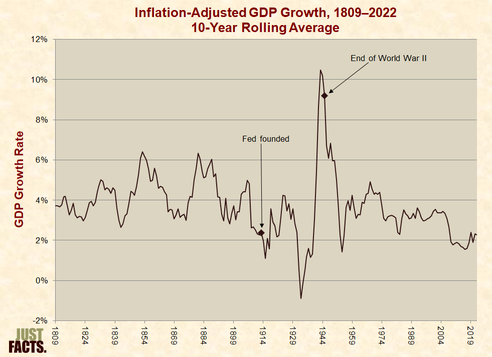
* In 1913, in response to a series of banking crises, the U.S. Congress established the Federal Reserve.[28]
* During World War I, many countries suspended the gold standard and began printing money to finance the war effort, which led to high inflation.[29] By 1919, the United States was the only world power that still followed the gold standard.[30]
* After World War I, Britain and other European countries briefly returned to the gold standard.[31]
* Britain left the gold standard in 1931 amidst the Great Depression, and the value of British money dropped significantly.[32] [33] Other nations that relied heavily on Britain for trade then dropped the gold standard to prevent Britain’s weak currency from pricing their “goods out of the large market which Britain provided.”[34]
* In 1934, the United States reduced the dollar’s value by raising the price of gold from $20.67 to $35 per ounce. The federal government also stopped allowing Americans to exchange their dollars for gold and confiscated privately-held gold.[35] [36] [37]
* In 1944, delegates from 44 nations met in Bretton Woods, New Hampshire to establish a new international monetary system. These countries agreed to value their currencies according to the U.S. dollar for international trade. In turn, the U.S. dollar would keep a fixed value of $35 per ounce of gold.[38]
* The Bretton Woods delegates also created the International Monetary Fund and the International Bank for Reconstruction and Development (now called World Bank Group) to help run the new system.[39]
* In 1971, Republican President Richard Nixon stopped allowing the exchange of dollars into gold, thus ending the Bretton Woods system. Most of the world’s currencies therefore had no link to a metal standard. Per the Federal Reserve Bank of Richmond:
* From 1965 to 1982, inflation in the United States increased multiplicatively during an era known as the Great Inflation. The annual inflation rate ranged from just over 1% in 1964 to over 14% in 1980.[41] [42] [43]
* In the early 1980s, the Federal Reserve enacted policies to raise private-sector interest rates. These high interest rates reduced inflation amid the recession of 1981–82.[44] [45] [46]
* The period from the mid-1980s to 2007 is known as the Great Moderation, when inflation stabilized and the economy expanded.[47] Part of this expansion took place in housing-related industries such as construction and mortgage borrowing.[48]
* From 1998 to 2006, home prices rose at unprecedented rates, and in 2007, they began to sharply decline.[49] As housing prices fell, financial institutions lost money because of borrowers defaulting on mortgages. These losses had “large spillover effects” on other parts of the economy. This led to the Great Recession that began in December 2007 and ended in 2009.[50] [51] [52]
* In response to the Great Recession, the Federal Reserve:
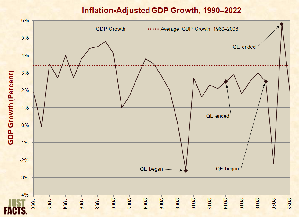
* Recovery from the Great Recession was a period of slow growth.[61] From 2010 to 2016, real (inflation-adjusted) gross domestic product (GDP) growth averaged 2.2% annually. From 1946 to 2007, the average annual growth rate was 3.2%.[62]
* During the Covid-19 outbreak of 2020—amid government-mandated shutdowns of businesses in nearly every state that cost millions of jobs[63] [64]—the Federal Reserve:
* A digital currency, virtual currency, or digital asset is a computerized representation of money. This includes traditional currencies that are transferred electronically and currencies that exist mainly in digital form.[74] [75]
* A virtual currency is stored and/or traded digitally but is not legally recognized by a government. Some, such as the gold that players earn in the online game World of Warcraft, cannot be converted into other currencies. Others, such as the now-defunct e-Gold, can be exchanged into traditional currencies. Most virtual currencies are centralized, meaning they have an administrator that controls its supply and makes rules for its use.[76] [77]
* Cryptocurrencies are a subset of virtual currencies that do not have central administrators. They use automated computer networks, instead of banks, to verify and process payments. Cryptocurrencies can be exchanged for traditional currencies.[78] [79] [80] [81] [82]
* In 2009, an anonymous computer programmer invented Bitcoin—the first cryptocurrency.[83] [84]
* Another cryptocurrency, XRP, was introduced by the company Ripple in 2012. It is primarily used as a currency to facilitate cross-border payments between banks.[85] [86]
* The computer network groups together a set of transactions, called a block. Computers across the network confirm the transactions contained in the block. Each block then becomes part of a shared public record—a block chain.[87] [88] [89]
* Because payment verifications are automated and recorded across an entire network, cryptocurrency trade is neutral and transparent.[90] [91] [92] [93]
* Cryptocurrency payments can be made at any time, since they do not rely on a third party bank for confirmation. They are also settled more quickly than traditional transactions. The process for a merchant to receive payment from a credit card transaction takes 24 to 72 hours. An average Bitcoin transaction takes 10 minutes, and an average XRP transaction takes four seconds.[94] [95] [96]
* Transactions using cryptocurrencies may have lower fees than traditional credit card transactions because they do not involve multiple intermediaries. In some cases, they have no transaction fee, whereas businesses typically pay 2% to 3% in fees to credit card companies.[97] [98] [99]
* The blockchain technology used in cryptocurrency transactions makes it nearly impossible to reverse payments. Businesses may see this as a benefit because they are not at risk for chargebacks by customers.[100] [101]
* The value of a virtual currency is not tied to a commodity such as gold and is not declared to be legal tender by the U.S. government.[102] [103] [104] [105] [106] Instead, it has value because people agree to use and accept it as payment.[107] [108]
* The value of a cryptocurrency can change quickly.[109] [110] [111] According to Lael Brainard, a member of the Federal Reserve’s Board of Governors:[112]
* Inflation is a general rise in prices for goods and services due to a decline in a currency’s value or purchasing power.[114] [115] [116]
* Inflation often occurs when governments create and circulate more money than needed by their nations’ economies. This causes the purchasing power of money to shrink and prices to increase.[117] [118] [119] [120] [121]
* Governments engage in inflationary policies to effectively tax citizens at higher rates and/or to default on their national debts.[122] [123] [124] [125]
* Per a 2002 speech by Ben Bernanke of the Federal Reserve:
* When governments create more money than needed by their economies, this doesn’t always raise the prices of consumer products and services. Instead, the additional money can inflate the prices of assets like stocks, real estate, and commodities. This is called “asset inflation,” and it increases the wealth of those who already own assets while making those assets less affordable for everyone else.[127] [128] [129] [130] [131]
* Government actions can have inflationary effects. For example:
* Market forces can have inflationary effects. For example:
* Deflation is the opposite of inflation—prices generally fall as the purchasing power of money increases.[138]
* Major causes of deflation or deflationary effects include the following:
* For facts about the “Inflation Reduction Act of 2022,” read this article from Just Facts.
* The Federal Reserve has recorded several measures of money in the U.S. economy:
* From 1959 to 2022, M2 and M3 relative to the size of the nation’s gross domestic product varied as follows:
* Inflation is typically measured by comparing prices for a wide range of goods and services over time.[151]
* The Federal Reserve mainly uses the Personal Consumption Expenditures (PCE) index—which is calculated by the U.S. Department of Commerce—to guide its policy decisions.[152]
* The Bureau of Labor Statistics calculates the Consumer Price Index (CPI), which is the most widely used measure of inflation. It affects the income of about 80 million people because it is used to adjust Social Security, food stamp, military retirement, and federal civil service retirement benefits. It is also used to determine school lunch prices and adjust the federal income tax code.[153]
* Although PCE and CPI follow the same general trends, there are differences between them:
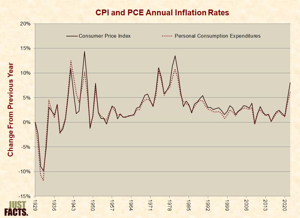
* From 1929 to 2022, the annual inflation rate as measured by CPI ranged from –9.9% to 14.4%, with a median of 2.8% and an average of 3.2%. During the same time period, the annual inflation rate as measured by PCE ranged from –11.8% to 12.5%, with a median of 2.5% and an average of 2.9%:
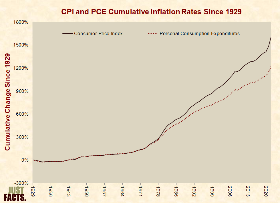
* From 1929 to 2022, the cumulative inflation rate was 1,611% as measured by CPI and 1,221% as measured by PCE:
* The Producer Price Index is a rough approximation of the wholesale prices paid by retailers for the products they sell to consumers.[162]
* From 1947 to 2022, the annual changes in consumer prices (CPI) and wholesale prices (PPI) varied as follows:
* From 1947 to 2022, the cumulative inflation rate was 1,212% as measured by CPI, 883% as measured by PCE, and 851% as measured by PPI:
* Wide variations in inflation can inflict serious damage on an economy.[165] [166] [167] [168] Per the U.S. Federal Reserve:
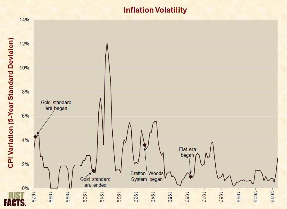
* Generally, periods of high inflation are associated with high volatility.[170] [171] [172]
* A key measure of inflation volatility is its standard deviation—or how widely inflation varies from its average over a specified time.[173] [174] [175]
* Since 1879, the 5-year standard deviation of the Consumer Price Index has varied as follows:
* Some individuals have claimed that the government’s indexes undercount inflation. These critics object to the following aspects of the government’s methodology:
* John Williams, founder of Shadow Government Statistics,[184] has claimed that the government undercounts inflation by 7% each year.[185]
* In 2008, the Bureau of Labor Statistics (BLS) published an article to address such criticisms. It presented the following facts:
* The Billion Prices Project is a non-government academic program that tracks price trends.[193] Its data—collected daily from thousands of online sources—shows a close correlation with government inflation data.[194]
* Inflation or deflation is most damaging if it changes rapidly and unexpectedly, which can inflict serious damage on an economy.[195] [196] [197]
* Unexpected inflation may hurt consumers because prices on goods can change daily, but wages do not always adjust immediately.[198]
* Unexpected inflation can hurt lenders, who are repaid with money worth less than when the terms of the loan were negotiated. This benefits borrowers because they repay their debts with less valuable money.[199]
* Since unexpected inflation can hurt lenders, it may make financial institutions less willing to make loans, particularly long-term loans.[200]
* Inflation also causes:
* When governments create more money than required by their economies, this doesn’t always raise the prices of consumer products and services. Instead, the additional money can inflate the prices of assets like stocks, real estate, and commodities. This is called “asset inflation.”[205] [206] [207] [208] [209] [210]
* Asset inflation can manifest in economic measures like:
* Asset inflation increases the wealth of those who already own assets, while making assets less affordable for people with little wealth.[220] [221] [222] [223] [224]
* Per the journal Environment and Planning, asset inflation:
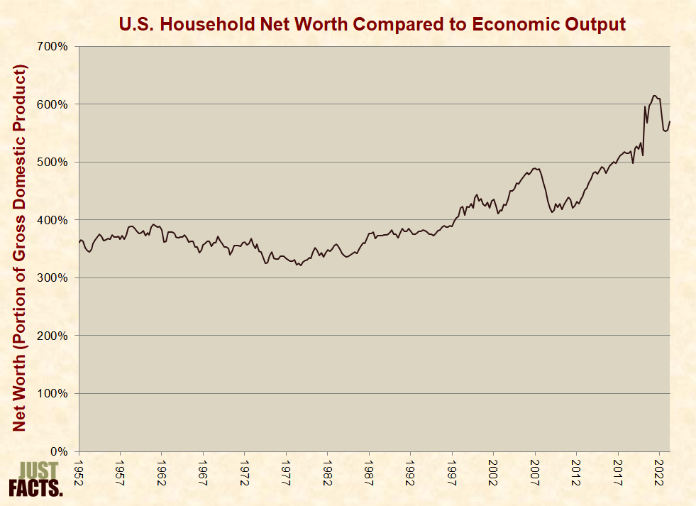
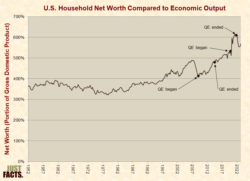
* One way to measure asset inflation is to compare a country’s net wealth to the size of its economy.[226] [227] From 2009 (when the Federal Reserve began a policy called quantitative easing) through the second quarter of 2023, this measure increased by 38%, or by 158 percentage points:
* During deflation, borrowers are less willing to take out loans because they will repay the lender with more valuable money.[230]
* Spending goes down during periods of deflation, because consumers wait for prices to drop even lower before making purchases or investments.[231] [232]
* Reduced spending and falling prices cause lower sales and profits. Lower demand for workers, and workers being unwilling to take pay cuts, can cause higher levels of unemployment.[233] [234]
* In periods of falling prices, the Federal Reserve takes action to reduce private-sector interest rates by reducing the federal funds rate—the interest rate banks charge each other for short-term loans. Lower interest rates encourage more borrowing and spending. This increases demand for products, which then leads to increased prices and wages.[235] [236]
* If the federal funds rate is near zero and there is still deflation, the Federal Reserve may employ quantitative easing. This means the Federal Reserve creates new money to purchase large quantities of assets, such as mortgage-related investments and federal bonds.[237] [238] In 2010, Federal Reserve Chairman Ben Bernanke said these purchases were made to “improve market functioning and to push longer-term interest rates lower.”[239] [240]
* The Federal Reserve used quantitative easing during the Great Depression of the 1930s, the Great Recession that began in 2007, and the Covid-19 pandemic of 2020.[241] [242] [243] [244] [245] [246] [247]
* A gold standard is a monetary system that defines a country’s currency as a fixed amount of gold. The government promises to exchange its currency into gold at a fixed rate.[248]
* If a country’s currency is not convertible into a commodity like gold, it is fiat money. Fiat money has value because a government declares that it is legal tender. The dollar’s status as legal tender is further supported by laws that requires tax debts to be paid in dollars. Its value is not tied to a commodity such as gold or silver.[249] [250]
* Historically, English money was known as “sterling,” and starting in the 10th century, 240 silver pennies made up one “pound sterling.”[251] In 1717, the United Kingdom’s Master of the Mint, Sir Isaac Newton, defined the pound sterling’s value in terms of gold rather than silver for the first time.[252]
* During the American Revolution, the Continental Congress issued paper money known as the “Continental.” It was not defined in terms of any precious metal and was easily counterfeited. Thus, it quickly lost its purchasing power, giving rise to the expression “not worth a Continental.”[253] [254]
* Starting with the Coinage Act of 1792, the United States used a bimetallic currency standard. This means the dollar was defined by its value in both silver and gold.[255]
* In December 1861, the United States suspended its link to a metal standard due to the costs of the Civil War.[256] Its currency was therefore fiat during this period.[257] In 1879, the U.S. government resumed converting paper currency into gold.[258] [259]
* In the early 19th century, Britain officially adopted the gold standard.[260] During the 1870s, Germany, Holland, Austro-Hungary, Russia, Scandinavia, and France also switched to the gold standard.[261]
* In 1900, the United States officially adopted the gold standard with the Gold Standard Act.[262]
* The period from 1880 to the outbreak of World War I in 1914 is known as the “classical gold standard” era.[263] During that time:
* During World War I, many countries suspended the gold standard and began printing money to finance the war effort, which led to high inflation.[269] By 1919, the United States was the only world power that still followed the gold standard.[270]
* After World War I, Britain and other European countries briefly returned to the gold standard.[271] During the Gold Exchange Era of 1925–1931, countries agreed to keep a supply of gold, U.S. dollars, or British pounds. The United States and United Kingdom agreed to hold gold.[272] [273]
* Britain left the gold standard in 1931 amidst the Great Depression, and the value of British money dropped significantly.[274] [275] Other nations that relied heavily on Britain for trade then dropped the gold standard to prevent Britain’s weak currency from pricing “their goods out of the large market which Britain provided.”[276]
* In 1944, delegates from 44 nations met in Bretton Woods, New Hampshire, to establish a new international monetary system. These countries agreed to value their currencies according to the U.S. dollar for international trade. In turn, the U.S. dollar would keep a fixed value of $35 per ounce of gold.[277]
* The Bretton Woods system required the United States to maintain a large supply of gold. In 1971, Republican President Richard Nixon ended the dollar’s link to gold.[278] Per the Federal Reserve Bank of Richmond:
* When the final gold link was severed in August 1971, the U.S. dollar and all other world currencies became fiat. Thus, their values began to rise and fall against one another based on supply and demand, financial speculation, and government currency manipulation.[280] [281]
NOTE: When interpreting the facts in this section, it is important to realize that association does not prove causation, and it is often difficult to determine causation in economics and other social sciences. This is because numerous variables might affect a certain outcome, and there is frequently no objective way to identify all of these factors and determine which is causing the others and to what degree.
* Under a strict gold standard, the amount of money in a country’s economy was determined by the amount of gold the government had in its possession. Prices were expected to remain stable if gold production kept up with the economy’s demand for money.[282] [283]
* Unexpected changes in the supply of gold were associated with short-term price instability.[284] [285] However, annual inflation rates in economies on a gold standard had long-term price stability.[286]
* When a country’s currency is fiat, the monetary policies of its central bank affect inflation. The Federal Reserve is responsible for deciding the amount of money in circulation and “maintaining confidence” in the currency’s value.[287] [288] [289] [290]
* During the classical gold standard era (1880–1914), the annual inflation rate in the U.S. averaged about 0.2% per year. From 1972 (after the end of the Bretton Woods System) to 2022, the average annual inflation rate was 4.0%:

* Wide variations in inflation can inflict serious damage on an economy.[292] [293] [294] [295] Per the U.S. Federal Reserve:
* A key measure of inflation volatility is its standard deviation—or how widely inflation varies from its average over a specified time.[297] [298] [299]
* During the classical gold standard era (1880–1914), the annual inflation rate in the U.S. had a standard deviation of 2.1%. From 1972 (after the end of the Bretton Woods System) to 2022, its standard deviation was 2.9%.[300]
* Since 1879, the 5-year standard deviation of the Consumer Price Index has varied as follows:
* Exchange rates—the prices of one currency in relation to others—play an important role in a country’s trade performance. They have large impacts on international trade and overall financial performance.[302] [303] For example:
* A country can influence exchange rates and its ratio of imports to exports by changing the value of its currency. In 1934, the U.S. reduced the dollar’s value in terms of gold by 69%. In 1949, the U.K. devalued the pound by 30%. In each of these cases, devaluing the currency encouraged exports by making the country’s goods cheaper for other countries to buy.[310] [311] [312] [313]
* When two countries’ currencies are defined in terms of the same material, such as gold, their exchange rate is fixed.[314] [315] For example, when the United States dollar and British pound were both valued in gold during the classical gold standard era (1880–1914), the exchange rate for £1 stayed steady at $4.86.[316]
* When countries do not have a common standard of value for their currencies, their exchange rates float. This means they fluctuate based on supply and demand, financial speculation, interest rates, and government currency manipulation.[317] [318]
* Since 1792, the U.S. dollar and British pound have alternated nine times between fixed exchange rates under the gold standard and floating exchange rates. During these periods, the British pound’s value against the dollar fluctuated as follows:

* In the centuries before 1971, the major economies generally used gold and silver coins for currency, and later, paper money backed by stockpiles of the precious metals.[322]
* In 1944, the Bretton Woods system was established with the U.S. dollar defined at $35 per ounce of gold. All other member countries set fixed exchange rates to the dollar.[323]
* In the 1960s, the U.S. struggled to maintain its role in the Bretton Woods system due to rising spending and inflation. In 1971, Republican President Richard Nixon suspended the government’s policy of exchanging dollars for gold in international markets, to stop the outflow of its gold supply. Within two years, exchange rates began to fluctuate.[324]
* Since 1973, member countries of the International Monetary Fund have chosen their own exchange rate systems. None of these countries are tied to a gold standard.[325]
* The International Monetary Fund (IMF) defines these exchange rate systems as:
* According to a 2023 report, the IMF has 190 member nations plus three territories, and Hong Kong and Macao. It classifies their exchange rate systems as follows:[330]
* The Federal Reserve was established in 1913 and serves as the central bank of the United States.[332]
* In 1775 during the Revolutionary War, the Continental Congress began printing paper money to finance the war. This currency was not backed by precious metals and was easily counterfeited. It quickly lost value, leading to the saying “not worth a Continental.”[333] [334]
* In 1788, the U.S. Constitution gave Congress the power to coin money, regulate its value, and punish those who counterfeit it.[335] [336]
* After the Constitution was ratified, Alexander Hamilton, the nation’s first treasury secretary, proposed the creation of a national bank. In 1791, the First Bank of the United States opened in Philadelphia.[337]
* The First Bank of the United States was authorized by Congress to hold $10 million in capital. It was mostly owned by private interests but was directed to serve a public purpose.[338] It made loans, accepted deposits, sold U.S. government bonds, and issued paper money backed by gold and silver.[339]
* In 1811, Congress did not renew the bank’s charter. Opponents of the national bank considered it unconstitutional and felt it infringed on states’ rights.[340] [341]
* From 1811 to 1816, state banks expanded and issued a wide variety of currencies.[342] These banks stopped backing their paper currencies with silver and gold, and the large volume of money that entered the economy caused the currencies to lose value. In order to fund the War of 1812, the federal government incurred large debts because the money it had lost its purchasing power.[343] [344]
* In 1816, Congress chartered the Second Bank of the United States. This bank redeemed state-issued paper money for gold and silver, which helped stem inflation.[345] [346] President Andrew Jackson considered the bank unconstitutional, and in 1836 he vetoed its re-charter.[347]
* The years from 1837 to 1863 are called the Free Banking Era. Private, state-chartered banks issued their own paper money without federal regulation. Although banks needed to follow state laws, government permission was not needed to open a bank.[348] [349] [350]
* The National Banking Act of 1863 established nationally chartered banks and required that they back their paper money with federal government bonds. The act was later amended to tax currencies issued by state banks. This reduced the amount of state-issued paper money and left the country with a uniform currency.[351] [352]
* From the end of the Civil War in 1865 to 1907, a series of bank panics caused many banks to fail. These panics occurred when a large number of customers withdrew their money out of fear that banks would run out of money.[353] [354] [355]
* In the same era, Canadian banks remained stable and again during the series of bank failures and panics that struck the United States in the 1920s and 1930s. Canadian banks were able to create multiple branches nationwide, which allowed them to spread risk across different markets. State-chartered banks in the United States were not allowed to cross state lines, and in some states, they were not allowed to create any branches.[356] [357] [358]
* Attempts in the United States to mirror the Canadian banking model failed until the 1980s, and full nationwide branch banking was not allowed until 1994. Groups such as farmers and small banks feared that branch banking would negatively affect their interests, and they argued that interstate banking violates states’ constitutional rights.[359] [360]
* In response to a bank panic in 1907, Congress established a Monetary Commission in 1908.[361] [362] The commission, led by Republican Senator Nelson Aldrich, made a plan to create a new central bank.[363] The plan, popularized in a book titled The Creature From Jekyll Island,[364] was criticized by progressives for giving control to bankers rather than the government.[365] [366]
* The Aldrich plan was abandoned when Democrat Woodrow Wilson, a founder of modern liberalism, became president of the United States.[367] In 1913, Wilson signed the Federal Reserve Act into law, creating a central banking system with a balance of power between government and private banks but giving the bulk of this power to government.[368] [369] [370] [371] [372]
* One provision of the Federal Reserve Act gave member banks a way to retire their paper currencies. This moved the country to a centrally controlled currency under the Federal Reserve (the Fed).[373] [374] [375]
* In 1927, Congress re-chartered the Federal Reserve ahead of schedule for an unlimited term. The Great Depression, which began in the United States in 1929, soon followed.[376] [377]
* Congress updated the Federal Reserve System with laws in:
* The Federal Reserve System is comprised of:
* The Board of Governors of the Federal Reserve:
* There are 12 regional Federal Reserve Banks,[390] and each:
* The Federal Open Market Committee:
* The Federal Reserve System is controlled by:
* The Board of Governors of the Federal Reserve:
* The Federal Reserve’s 12 regional Reserve Banks are separately incorporated,[412] and each has a:
* Congress established the Federal Reserve’s authority in 1913.[420] The Fed is governed by federal laws, including those that require:
* In 2023, U.S. Congressman Thomas Massie (R–KY) introduced the Federal Reserve Transparency Act. It would allow audits on areas of the Fed that are currently restricted, including policy decisions and international transactions.[446]
* The Federal Reserve System has five main responsibilities:
* “Monetary policy” refers to the Fed’s actions to achieve three goals set by Congress: maximum employment, stable prices, and moderate long-term interest rates. The Fed’s monetary policies directly affect interest rates, which in turn, affect credit flows, stock prices, exchange rates, business investments, employment, inflation, and other aspects of the economy.[449]
* One of the main ways in which the Federal Reserve implements monetary policy is by influencing the federal funds rate, which is the interest rate that banks charge each other for short-term loans. This rate has wide-ranging ripple effects on the economy.[450] [451]
* Prior the Great Recession of 2007–2009,[452] [453] the Federal Reserve influenced the federal funds rate primarily by ordering the New York Federal Reserve Bank to buy or sell government bonds on the open market.[454] [455] [456] When the Federal Reserve sought to:
* During the Great Recession and the Covid-19 pandemic, the Federal Reserve took actions that caused banks to have excessive amounts of money to lend. This made the previous methods of influencing the federal funds rate ineffective.[459] [460] [461] [462]
* Since the Great Recession, the Federal Reserve has mainly influenced the federal funds rate by paying interest to banks and other financial institutions to store money at regional Federal Reserve Banks.[463] [464]
* From 1954 to 2023, the federal funds rate ranged from 0% to 19%, with an average of 5% and median of 4%:

* Until 2020,[466] the Federal Reserve also implemented monetary policy by requiring member banks to keep a specific portion of the money their customers deposited in cash (either in their own vaults or at regional Federal Reserve Banks). When the Board of Governors allowed banks to decrease this portion, banks could loan more money to the public, which caused more money to circulate through the economy.[467] [468]
* The Federal Reserve stopped requiring banks to keep a specific portion of their assets in cash during 2020 after the following events:
* Since the start of the Federal Reserve policy of paying interest to banks on cash they store at regional Federal Reserve Banks, rates have varied as follows:
* From 1973 to 2023, the total cash assets of commercial banks relative to their liabilities ranged from 3% to 22%, with a median and average of 10% .
* The Federal Reserve also implements monetary policy through the following mechanisms:
* In addition to conducting monetary policy, Federal Reserve Banks provide services to:
NOTE: When interpreting the facts in this section, it is important to realize that association does not prove causation, and it is often difficult to determine causation in economics and other social sciences. This is because numerous variables might affect a certain outcome, and there is frequently no objective way to identify all of these factors and determine which is causing the others and to what degree.
* The Federal Reserve has three priorities set by Congress in 1977: (1) maximum employment, (2) stable prices, and (3) moderate long-term interest rates.[500] [501]
* World War I began in 1914, less than one year after the Federal Reserve System was created. The war created tremendous upheaval in the international financial system, including the suspension of the international gold standard, major increases in government debt, and soaring inflation.[502] [503] [504]
* The interwar years from 1919 to 1939 were a time of financial chaos. After World War I, European nations tried to restore the pre-war gold standard but abandoned it amidst the Great Depression.[505]
* The Great Depression was more severe and longer-lasting in the United States than in many other countries. Some economists believe the Fed’s policies from 1929 to 1937 contributed to the country’s economic problems.[506] [507]
* During World War II, the Federal Reserve focused on financing the United States’ war efforts. This focus diverted the Federal Reserve from its primary mission.[508]
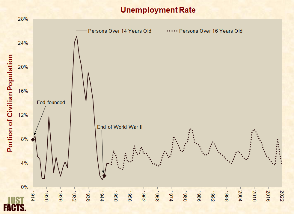
* The forthcoming facts about unemployment, inflation, interest rates, and economic growth cover the Federal Reserve’s tenure from 1914 (when available) to the latest available data. They also isolate the post-World War II period (1946–present) to remove the impact of the two world wars and the Great Depression. When available, data from the period prior to the Fed’s creation in 1913 is also provided.
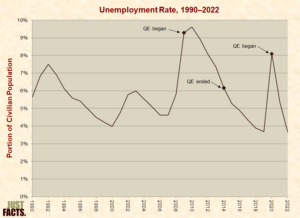
* During the Fed’s tenure, the average annual unemployment rate has ranged from 1% to 25%, with a median of 6% and an average of 7%. Post-World War II, the average annual unemployment rate has ranged from 3% to 10%, with a median and an average of 6%:
* Stable prices occur when the economy is not experiencing high or unexpected rates of inflation or deflation.[512] [513] [514]
* The average inflation rate:

* Wide variations in inflation can inflict serious damage on an economy.[521] [522] [523] [524] Per the U.S. Federal Reserve:
* A key measure of inflation volatility is its standard deviation—or how widely inflation varies from its average over a specified time.[526] [527] [528]
* Inflation’s standard deviation:
* Since 1879, the 5-year standard deviation of the Consumer Price Index has varied as follows:
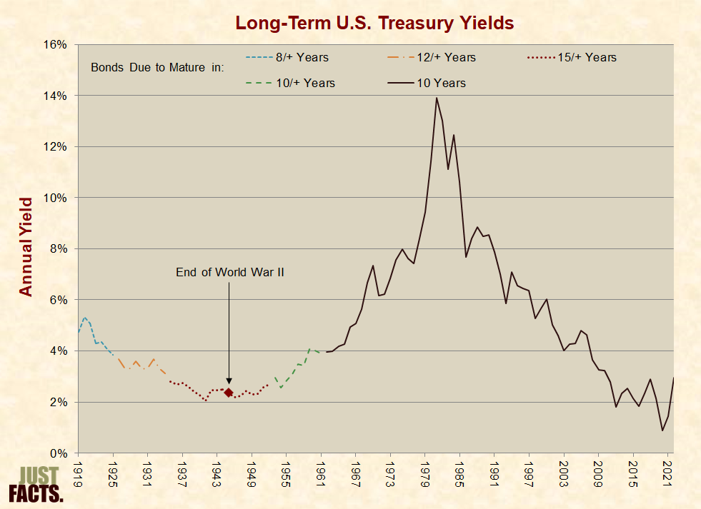
* Low interest rates help encourage spending in the economy by making it cheaper to borrow money.[533] [534]
* For the Fed’s tenure starting in 1919, annual interest rates on long-term federal bonds have ranged from 1% to 14%, with an average of 5% and a median of 4%. Post-World War II, they have ranged from 1% to 14%, with an average and a median of 5%:[535]
* Gross domestic product (GDP) measures the value of the goods and services produced by an economy during a specific time period. GDP is defined by the equation: Hours worked × Labor productivity.[538] [539]
* The growth rate of inflation-adjusted GDP is a key indicator of the health of an economy. A strong growth rate is often associated with higher rates of employment, while low or negative rates may accompany employment declines.[540]
* Average annual inflation-adjusted GDP growth was 4.0% prior to the Fed’s creation, 3.3% during the Fed’s full tenure, and 2.9% post-World War II:
* Quantitative easing is an unconventional Federal Reserve policy implemented during the Great Depression of the 1930s, the Great Recession that began in 2007, and the Covid-19 pandemic of 2020.[542] [543] [544] [545] [546] [547] [548] [549]
* During recessions, the Federal Reserve seeks to encourage economic activity by enacting policies to reduce the federal funds rate, which is the interest rate that banks charge each other for short-term loans. This rate has wide-ranging ripple effects on the economy.[550] [551] [552]
* From 1998 to 2006, home prices rose at unprecedented rates, and in 2007, they began to sharply decline.[553] As housing prices fell, financial institutions lost money because of borrowers defaulting on mortgages. These losses had “large spillover effects” on other parts of the economy. This led to the Great Recession that began in December 2007 and ended in 2009.[554] [555] [556]
* In a financial crisis like the Great Recession, the Federal Reserve may push the federal funds rate close to zero, as it did in December of 2008. Since the rate could not be reduced any further, and economic conditions did not improve, the Federal Reserve implemented quantitative easing.[557]
* During the quantitative easing of the Covid-19 pandemic, the Fed created trillions of dollars of new money to purchase financial assets, such as:[563] [564] [565]
* The stated purpose of quantitative easing (QE) during the Great Recession was to help the economy by reducing interest rates.[568]
* In January 2009, as the Fed initiated QE, then-Federal Reserve Chairman Ben Bernanke said the program’s main purpose was to make it easier and less costly for households and businesses to borrow money. “If the program works as planned,” he said, “it should lead to lower rates and greater availability of consumer and small business credit.”[569] [570] [571]
* With easier and cheaper access to credit, businesses are able to make investments, such as buying new equipment. Per an article published by the Federal Reserve Bank of St. Louis in 2011, “over time, new business investments should bolster economic activity, create new jobs, and reduce the unemployment rate.”[572]
* By making large-scale purchases of long-term federal debt, the Fed reduced the amount of debt available for sale to the public, which placed downward pressure on interest rates.[573] [574]
* The Fed also purchased mortgage-related investments and debt from government-sponsored enterprises like Fannie Mae, Freddie Mac, and the Federal Home Loan Banks. The purpose of these purchases was to reduce mortgage rates in order to support the housing sector.[575] [576] Chairman Bernanke said that “bringing down mortgage rates” stimulates “home-buying, construction, and related industries.”[577]
* Bernanke also stated that the Fed was “compelled” to implement QE because “many financial institutions” had incurred “substantial losses” in the housing market crash, and these firms still owned a “large quantity” of “troubled” and “illiquid assets of uncertain value.” These were called “toxic assets” and consisted largely of subprime and other high-risk mortgages that had fueled the housing boom and subsequent crash.[578] [579] [580] [581]
* Since financial institutions had suffered large losses and still owned stockpiles of bad investments that they could not sell without taking further losses, these firms could not effectively loan, borrow, or trade. Bernanke said this was problematic because “our economic system is critically dependent on the free flow of credit.”[582]
* In order to open the flow of credit, the Fed began purchasing toxic assets from financial institutions and providing large loans to these firms. This provided the firms with additional cash and “reduced the total amount of risky assets investors held.”[583] [584] [585]
* As the Fed began implementing QE, Chairman Bernanke stated that:
* When the Fed implemented QE during the Covid-19 pandemic of 2020, Federal Reserve Chairman Jerome Powell said the program’s main purpose was to “safeguard financial markets” and:
* At the beginning of the Great Recession, the Federal Reserve set up an emergency lending program to stimulate the flow of money in the economy. From December 2007 to September 2008, the Fed funded loans to banks and financial firms by selling off $315 billion of its federal bonds.[590] [591] [592]
* In September 2008, the Fed ran out of federal bonds to sell but continued to make loans by creating new money. These new loans increased the Fed’s assets from less than $1 trillion to over $2 trillion in approximately 3 months. Fed Chairman Ben Bernanke referred to this policy as “credit easing.”[593] [594]
* In November 2008, the Federal Reserve announced its plan to begin a quantitative easing (QE) program. The original plan was to purchase large amounts of mortgage-related investments and debt belonging to housing-related government-sponsored enterprises like Fannie Mae, Freddie Mac, and the Federal Home Loan Banks. The stated goal was to make mortgages cheaper and more available to the public.[595]
* In March of 2009, the Fed announced its plan to expand the size and scope of its purchases to include long-term government debt. The stated goal was to help improve credit conditions outside of the housing industry.[596]
* From March 2009 to March 2010, during what is now called QE1, the Fed purchased:
* Due to continued low inflation and economic weakness, the Federal Reserve initiated a second round of large-scale asset purchases called QE2. From November 2010 to June 2011, it purchased $600 billion of long-term federal debt.[599]
* From September 2011 to December 2012, the Fed implemented a Maturity Extension Program, which is also known as “Operation Twist.” The Fed sold short-term bonds and purchased an equal amount of long-term federal bonds. The goal was to reduce long-term interest rates without further expanding the Fed’s balance sheet.[600] [601]
* In September 2012, the Fed began QE3—a phase of large-scale asset purchases without a set end date or total cost estimate. It began purchasing $40 billion of mortgage-related investments each month, then in January 2013 added $45 billion of long-term federal bonds per month. Monthly purchases were tapered down until QE3 ended in October 2014 with a total cost of approximately $1.6 trillion.[602] [603] [604]
* In March 2020, the Fed responded to the Covid-19 pandemic and state government shutdowns of “nonessential businesses” with an effective QE.[605] [606] [607] Per Fed Chairman Jerome Powell: [608]
* From the inception of the Federal Reserve in 1913 through 2007,[610] the Fed accumulated $1.3 trillion of inflation-adjusted net assets. Due to QE and related policies that the Fed has implemented since then, its assets grew:
* From the inception of the Federal Reserve in 1913 through 2007,[616] the Fed accumulated net assets equal to 6% of the nation’s annual economic output, or gross domestic product (GDP). Due to QE and related policies that the Fed has implemented since then, its assets grew:
[617] [618] [619] [620] [621] [622]
* Since 1933, the portion of the national debt borrowed from the Federal Reserve has varied as follows:

NOTE: When interpreting the facts in this section, it is important to realize that association does not prove causation, and it is often difficult to determine causation in economics and other social sciences. This is because numerous variables might affect a certain outcome, and there is frequently no objective way to identify all of these factors and determine which is causing the others and to what degree.
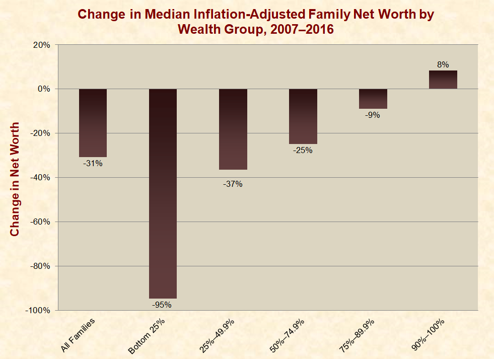
* Net worth is the difference between people’s assets and liabilities.[627]
* From 2007 to 2016, during and after the Great Recession and implementation of quantitative easing, the inflation-adjusted median net worth of U.S. families declined for all wealth groups except the top 10%:
* Market income consists of non-government income, such as labor income, business income, and capital gains.[629]
* From 2007 to 2016, during and after the Great Recession and implementation of quantitative easing, inflation-adjusted market income for the:
* From 2007 to 2016, during and after the Great Recession and implementation of quantitative easing, the annual unemployment rate fell from about 5% to about 4%:
* The labor force participation rate is the portion of people aged 16 and older who are “either working or actively seeking work.”[640] [641] [642]
* From 2007 to 2016, during and after the Great Recession and implementation of quantitative easing, the annual labor force participation rate fell from 66% to 63%:

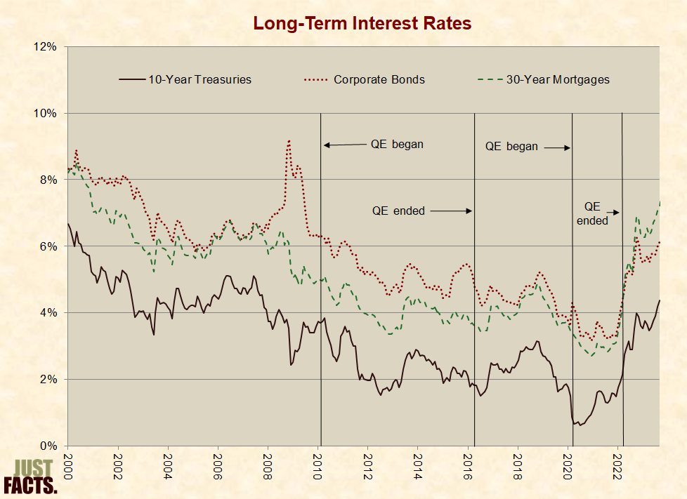
* Mortgage rates began declining when the Federal Reserve announced its plan to purchase mortgage-related investments in November of 2008, even though it had not made any purchases yet.[646] [647]
* From 2007 to 2016, during and after the Great Recession and implementation of quantitative easing, interest rates on:
* Inflation is a general rise in prices for goods and services due to a decline in a currency’s value or purchasing power.[652] [653] [654] The most widely used measure of inflation is the Consumer Price Index (CPI).[655]
* In 2009, the annual change in CPI dropped below zero to –0.4%. Inflation since 2010 has been positive, which offset fears of a deflationary crisis.[656] [657]
* Some economists worried that the money created during QE would cause high inflation.[658] [659] However, from 2007 to 2016, the average inflation rate was lower than the 10-year rolling average over the preceding 4 decades:
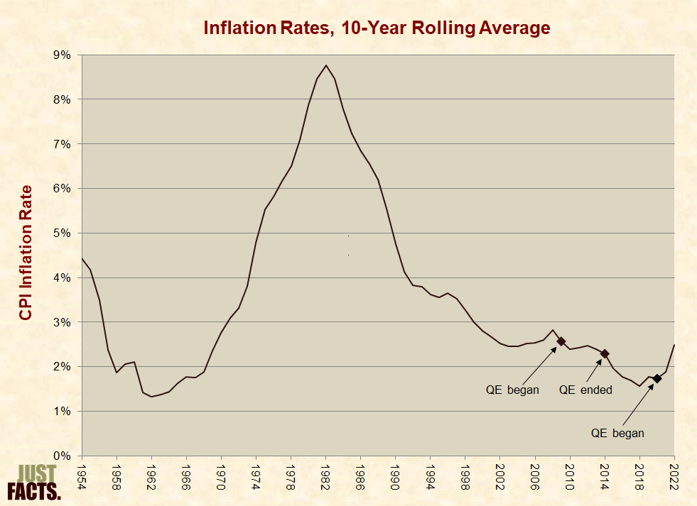
* Inflation likely remained low because the newly created money stayed in banks’ reserves and was not circulated into the economy. If banks begin loaning out these funds, the money supply will expand, and inflation may increase.[663] [664] [665] [666]
* When governments create more money than required by their economies, this doesn’t always raise the prices of consumer products and services. Instead, the additional money can inflate the prices of assets like stocks, real estate, and commodities. This is called “asset inflation.”[667] [668] [669] [670] [671]
* Since quantitative easing’s purpose is to reduce interest rates,[672] its implementation may cause asset inflation. For instance, lower interest rates result in:
* Asset inflation can manifest in economic measures like:
* Asset inflation increases the wealth of those who already own assets, which makes those assets less affordable for others.[688] [689] [690] [691] [692]
* Per the journal Environment and Planning, asset inflation:
* One way to measure asset inflation is to compare a country’s net wealth to the size of its economy.[694] [695] Since 2007, the total net worth of U.S. households has increased from 488% of the nation’s annual economic output to 571%:
* Gross domestic product (GDP) measures the value of the goods and services produced by an economy during a specific time period. GDP is defined by the equation: Hours worked × Labor productivity.[701] [702]
* From 2007 to 2016, during and after the Great Recession and implementation of quantitative easing, inflation-adjusted economic growth did not reach its average of 3.4% over the prior half century:
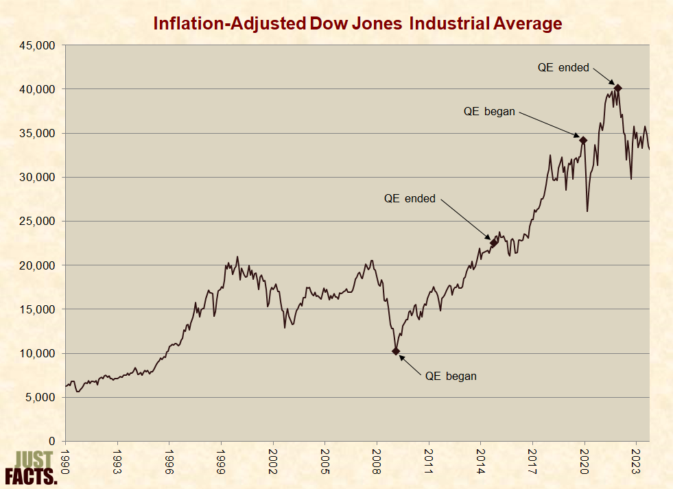
* The Dow Jones Industrial Average is an indicator that measures the value of a group of large, fiscally sound U.S. companies from various industries.[706] [707]
* From 2007 to 2016, during and after the Great Recession and implementation of quantitative easing, the Dow Jones inflation-adjusted average rose about 18%:[708]
* In 2021, Democratic President Joe Biden asserted he was “very fastidious about not talking to” the Federal Reserve in order to maintain the Fed’s independence.[713]
* In 2021, Biden nominated Jerome Powell to a second term as chair of the Federal Reserve in order to ensure “stability and independence” at the Fed.[714] [715]
* In 2022, amid rapidly rising inflation,[716] Biden reiterated the Fed’s “primary responsibility to control inflation” and that he “won’t meddle with the Fed, but” he “will tackle high prices.”[717] [718]
* As a 2016 presidential candidate, Republican Donald Trump criticized the Federal Reserve, saying that it had created “a big, fat, ugly bubble,” and was supporting “a very false economy” with its policies.[719]
* In a 2015 interview, Trump stated that the United States used to be solid “because it was based on a gold standard.” He also stated that it would be difficult to implement the gold standard “at this point” because “we do not have the gold.”[720]
* After taking office, Trump repeatedly said he doesn’t like a “strong” dollar, meaning he doesn’t want the exchange rate to rise excessively.[721] [722]
* In 2017, Trump named Jerome Powell to chair the Federal Reserve. Powell expected to continue the policies put in place by his predecessors.[723] [724]
* In 2019, prior to the Covid-19 pandemic and economic recession,[725] [726] Trump urged the Fed to lower interest rates and resume quantitative easing to boost the economy.[727] [728] [729]
* Senator Rand Paul (R-KY) has criticized the Federal Reserve’s actions during the financial crisis. In 2016, he wrote that the Fed’s power has been “unchecked” and “arguably unconstitutional.”[730]
* Paul proposed legislation in 2011, 2013, 2015, 2017, 2019, 2021, and 2023 entitled the Federal Reserve Transparency Act and commonly known as “Audit the Fed.” Each version of the bill would require the Government Accountability Office to complete an audit of the Federal Reserve Board and Federal Reserve banks.[731] [732] [733] [734] [735] [736] [737]
* In 2020, then Senate Minority Leader Charles “Chuck” Schumer (D-NY) stated that the Fed “must make decisions on an objective economic analysis and judgement.”[738] [739]
* In 2017, Schumer was disappointed when Fed Chairwoman Janet Yellen was not nominated for a second term. He previously advocated for her original nomination in 2013.[740] [741]
* In 2014, Schumer stated that the Federal Reserve should “be careful” about raising interest rates because of the “overwhelming problem” of slow job growth.[742]
* Schumer supported Ben Bernanke’s nomination as chairman in 2005 and later applauded Bernanke’s “steady hand” during the financial crisis.[743] [744]
* Schumer has voted against the “Audit the Fed” bill.[745]
* Senator Ted Cruz (R-TX) cosponsored the 2013 and 2015 “Audit the Fed” bills.[746] [747]
* During a November 2015 Republican presidential debate, Cruz referred to the Federal Reserve as “philosopher kings” and called for “sound money and monetary stability, ideally tied to gold.”[748]
* In a December 2015 hearing with Chairwoman Janet Yellen, Cruz blamed the Federal Reserve’s policies for the 2008 financial crisis.[749]
* Senator Bernie Sanders (I-VT) has criticized the Federal Reserve, calling it a “rigged economic system.” In 2015—when he was a candidate for the Democratic presidential nomination—he wrote that the Fed should undergo a “full and independent audit” every year. He further wrote that “banking industry executives” serving on the Fed’s boards have “conflicts of interest” and should be replaced with “representatives from all walks of life.”[750]
* Sanders has also criticized actions of the Fed. For example, he disagreed with the Fed’s decision to begin raising interest rates in 2015 while unemployment was still over 4%. Rather than paying interest to banks, he proposed that the Fed should charge the banks “a fee that would be used to provide direct loans to small businesses.”[751]
* In 2009, Democratic President Barack Obama nominated Ben Bernanke for a second term as Chairman of the Federal Reserve Board. Bernanke was first appointed by Republican President George W. Bush.[752]
* At the end of Bernanke’s term, Obama nominated Janet Yellen as Chairwoman of the Federal Reserve Board.[753]
* During his tenure, Obama defended the Fed’s quantitative easing program.[754] His administration opposed the 2015 “Audit the Fed” legislation.[755] [756]
* In 2015, U.S. Rep. Kevin Brady (R-TX) introduced a bill that would establish a Centennial Monetary Commission. The Commission would assess the Federal Reserve’s historical impact on the U.S. economy and recommend policies for the future.[757]
* In 2012, Brady proposed the Sound Dollar Act, which would have limited the Fed’s priorities to promoting long-term price stability and establishing a way to measure whether that goal is achieved.[758]
* U.S. Rep. Bill Huizenga (R-MI) proposed the Fed Oversight Reform and Modernization (FORM) Act of 2015. It would require the Federal Reserve to adopt a rules-based monetary policy of its choosing. The Fed could stop following the rule, provided it explains its decision to Congress.[759]
* In 2013, U.S. Rep. Nancy Pelosi (D-CA) supported Janet Yellen’s nomination as Chairwoman of the Federal Reserve, and in 2017 praised Yellen’s tenure. Pelosi called on Yellen’s successor, Jerome Powell, to continue Yellen’s policies.[760] [761]
* Pelosi opposes “Audit the Fed” bills, saying in a 2012 press conference that Congress should not monitor the Federal Reserve “in terms of monetary policy.”[762]
* As a candidate for the Republican presidential nomination in 2011, former Speaker of the House Newt Gingrich heavily criticized the Federal Reserve. He partially blamed the Federal Reserve Board for the Great Recession and weak recovery. He also promised to fire its leadership, demand a full audit, and limit their mandate.[763] [764] [765]
* Gingrich advocated creating a gold commission—similar to the one convened under President Reagan—to consider reinstating a gold standard.[766]
* In a February 2018 commentary, Gingrich warned that the Fed’s attitude and policies will obstruct economic growth.[767]
* In 2008, U.S. Rep. Paul Ryan (R-WI) proposed legislation to set price stability as the Fed’s sole long-term goal, which would eliminate full employment from the Fed’s dual mandate.[768]
* In 2009, Ryan wrote that the Federal Reserve should base monetary policy on a set of “commodities” or should “explicitly embrace inflation” goals.[769]
* Democratic President Bill Clinton nominated Reagan appointee Alan Greenspan to a third term as Federal Reserve chairman in 1996.[770] In 2000, he nominated Greenspan again.[771]
* In 1993, the Clinton administration made a policy not to comment on or interfere with the Federal Reserve’s policies and actions.[772] [773]
* In 1994, Clinton signed the Riegle–Neal Interstate Banking and Branching Efficiency Act into law. This law made it easier for banks to open branches and acquire other banks across state lines. He praised the act for helping banks “better meet the needs of our people.”[774]
* Steve Forbes, the editor of Forbes magazine, ran for president as a Republican in 1996 and 2000, advocating for using the gold price to guide U.S. monetary policy.[775] [776] [777]
* Forbes critiques monetary and exchange rates policy in his column, and in 2014 released the book Money: How the Destruction of the Dollar Threatens the Global Economy—and What We Can Do About It.[778] [779]
* During his campaign for the 1980 presidential election, Republican Ronald Reagan called for a return to the gold standard.[780] He was quoted as believing that “no great nation in history that went off the gold standard remained great.”[781]
* As president, Reagan supported the creation of the U.S. Gold Commission, which in 1982 recommended against restoring the gold standard.[782]
* Reagan publicly supported the Federal Reserve’s unpopular policy decisions during the recession of 1981–82. These policies effectively ended The Great Inflation.[783] [784] [785] [786]
* In 1980, Congress voted to create the U.S. Gold Commission to study whether to reinstate a gold standard in the United States. Senator Jesse Helms (R-NC) and U.S. Rep. Ron Paul (R-TX) sponsored the measure.[787]
* The commission majority report rejected restoring a monetary link between the dollar and gold.[788] Paul co-authored the commission’s minority report, which argued for restoring a gold link. The report was released as a book, The Case for Gold.[789] [790]
* In 2011, Paul sponsored a bill to repeal the Federal Reserve Act and abolish the Federal Reserve Board and banks.[791]
* Paul highlighted his critique of the Federal Reserve during his runs for president and authored the book End the Fed.[792] [793]
* U.S. Rep. Jack Kemp (R-NY), also U.S. Housing Secretary and 1996 vice presidential candidate, advocated for using the price of gold to guide monetary policy.[794] [795]
* In 1984, Kemp introduced legislation to define the dollar relative to gold and require the Treasury to exchange gold for dollars.[796]
[1] Article: “Money.” Encyclopedia Britannica, 1998. <www.britannica.com>
“A commodity accepted by general consent as a medium of economic exchange. It is the medium in which prices and values are expressed; as currency, it circulates anonymously from person to person and country to country, thus facilitating trade, and it is the principal measure of wealth.”
[2] Textbook: Macroeconomics (6th edition). By N. Gregory Mankiw. Worth Publishers, 2006.
Pages 77–78:
Money has three purposes. It is a store of value, a unit of account, and a medium of exchange.
As a store of value, money is a way to transfer purchasing power from the present to the future. If I work today and earn $100, I can hold the money and spend it tomorrow, next week, or next month. Of course, money is an imperfect store of value: if prices are rising, the amount you can buy with any given quantity of money is falling. Even so, people hold money because they can trade the money for goods and services for some time in the future.
As a unit of account, money provides the terms in which prices are quoted and debts are recorded. Microeconomics teaches us that resources are allocated according to relative prices—the prices of good relative to other goods—yet stores post their prices in dollars and cents. A car dealer tells you that a car costs $20,000, not 400 shirts (even though it may amount to the same thing). Similarly, most debts require the debtor to deliver a specified number of dollars in the future, not a specified amount of some commodity. Money is the yardstick with which we measure economic transactions.
As a medium of exchange, money is what we use to buy goods and services. “This note is legal tender for all debts, public and private” is printed on the U.S. dollar. When we walk into stores, we are confident that the shopkeepers will accept our money in exchange for the items they are selling.
[3] Webpage: “All About Money.” European Commission. Accessed June 3, 2018 at <ec.europa.eu>
“Many thousands of years ago, our European ancestors lived as hunters and farmers. They did not have the banknotes and coins that we use today. Instead, they would exchange goods with each other: for example, a hunter could exchange animal skins with a farmer for grain, or a fisherman could exchange decorative seashells for a polished stone axe with a hunter. This exchange is known as barter.”
Pages 9–10:
Throughout by far the greater part of man’s development, barter necessarily constituted the sole means of exchanging goods and services. …
Commodities were chosen as preferred barter items for a number of reasons—some because they were conveniently and easily stored, some because they had high value densities and were easily portable, some because they were more durable (or less perishable).
[5] Webpage: “The Story of Money: 02—Common Products as Money.” Federal Reserve Bank of Atlanta. Accessed August 8, 2017 at <www.frbatlanta.org>
“Trading everyday items made barter easier. It reconciled the wants of buyer and seller, simplified payments, and introduced standard measures. Common goods used in trade are known as commodity money. Cows as a form of money … Tea as a form of money … Raw metals as a form of money.”
[6] Webpage: “The Story of Money: 03—Value in Use, Value in Exchange.” Federal Reserve Bank of Atlanta. Accessed August 8, 2017 at <www.frbatlanta.org>
In some forms, money has value in use: you can eat or wear it, chop wood with it, or use it to make something else. In other forms, money has value in exchange: it works because we agree that the money represents a certain value. The silver in this “tiger tongue” made it intrinsically valuable. This Luristan bronze arm ring is a 7,000-year-old form of money. Dried grain was useful as money and food. Arrowheads were popular in trade. Throwing knives were used in the Congo as tools and money. Cowrie shell necklaces were used for jewelry and exchange. Kissi pennies are still used in parts of West Africa.
[7] Textbook: Macroeconomics (6th edition). By N. Gregory Mankiw. Worth Publishers, 2006.
Page 78: “To better understand the functions of money, try to imagine an economy without it: a barter economy. In such a world, trade requires the double coincidence of wants—the unlikely happenstance of two people each having a good that the other wants at the right time and place to make an exchange. A barter economy permits only simple transactions.”
[8] Webpage: “Cowry Shells, a Trade Currency.” By Ingrid Van Damme. Museum of the National Bank of Belgium, January 11, 2007. <www.nbbmuseum.be>
Long before our era the cowry shell was known as an instrument of payment and a symbol of wealth and power. This monetary usage continued until the 20th century. …
The cowry which is indigenous in the warm waters of the Indian and Pacific Oceans travelled by land and by sea and gradually spread out its realm. It became the most commonly used means of payment of the trading nations of the Old World. The cowry was accepted in large parts of Asia, Africa, Oceania and in some scattered places in Europe. Chinese bronze objects, the oldest dating back to the 13th century B.C., inform us about this monetary usage. This tradition has also left its traces in the written Chinese language.
[9] Book: A History of Money: From Ancient Times to the Present Day (3rd edition). By Glyn Davies. University of Wales Press, 2002.
Page 46: “The Chinese at the end of the Stone Age began for instance to manufacture both bronze and copper ‘cowries’; and these dumpy imitations, which must have represented very high values at least when they were first introduced, are considered by some numismatists to be among the earliest examples of quasi-coinage, although this depends on how strictly one defines the term.”
Page 56:
We have already noted how metal cowries, of bronze or copper, were cast in China as symbols of objects already long accepted as money. A similar process took place with regard to spades, hoes and adzes (variants of the most common tools) and also of knives. The common characteristic of all these metallic moneys was not only that they were cast but that they were almost invariably composed of base metals.
[10] Article: “The Importance of the Lydian Stater as the World’s First Coin.” By Everett Millman. World History Encyclopedia, March 27, 2015. <www.worldhistory.org>
The Lydian Stater was the official coin of the Lydian Empire, introduced before the kingdom fell to the Persian Empire. The earliest staters are believed to date to around the second half of the 7th century BCE, during the reign of King Alyattes (r. 619–560 BCE). According to a consensus of numismatic historians, the Lydian stater was the first coin officially issued by a government in world history and was the model for virtually all subsequent coinage.
[11] Webpage: “The Origins of Coinage.” British Museum. Accessed August 8, 2017 at <www.britishmuseum.org>
The earliest coins are found mainly in the parts of modern Turkey that formed the ancient kingdom of Lydia, but are made from a naturally occurring mixture of gold and silver called electrum. …
Although irregular in size and shape, these early electrum coins were minted according to a strict weight-standard. The denominations ranged from one stater (weighing about 14.1 grams) down through half-staters, thirds, sixths, twelfths, 1/24ths and 1/48ths to 1/96th stater (about 0.15gm).
[12] Book: A History of Money: From Ancient Times to the Present Day (3rd edition). By Glyn Davies. University of Wales Press, 2002.
Page 66:
From its birthplace in Lydia and Ionia the knowledge and use of coins spread rapidly east into the Persian empire and west through the rest of the Ionian and Aegean islands to mainland Greece, and then to its western colonies, especially Sicily. It also spread northward to Macedonia, Thrace and the Black Sea, but it was only partially, reluctantly and belatedly accepted in Egypt. Mainland Italy also was at first rather slow in accepting the Greek financial innovations, in contrast to the speed with which they were adopted by Sicily. Apart from these two limited exceptions of mainland Italy and Lower Egypt, the use of coinage spread rapidly around the countries bordering the central and eastern Mediterranean and over the widespread and growing Persian empire through Mesopotamia into India. …
The rapid eastward spread of coins from Lydia was not so much because of Lydian traders going east but rather a case of the spoils of war through the Persians moving quickly west.
[13] Book: A History of Money: From Ancient Times to the Present Day (3rd edition). By Glyn Davies. University of Wales Press, 2002.
Pages 106–107:
Shortly following Diocletian’s abdication in 305 Constantine took over an initially disputed control of much of the western empire in 306, and eventually established his authority throughout the empire…. Early in Constantine’s reign he issued a coin that is in some ways the most famous single coin in history—the gold solidus, which was to be produced, at a rate of 72 to the pound weight, for some seven hundred years. No other coin has remained pure and unchanged in weight for anything like so long a period, for when Rome fell it continued to be issued from the Byzantine capital….
[14] Book: A History of Money: From Ancient Times to the Present Day (3rd edition). By Glyn Davies. University of Wales Press, 2002.
Page 125: “The first true English penny … thus dates from 765. However, it was Offa’s conquest of Kent … that enabled Offa so to increase the production of these magnificent coins that their fame soon spread all over northern Europe….”
[15] Book: A History of Money: From Ancient Times to the Present Day (3rd edition). By Glyn Davies. University of Wales Press, 2002.
Pages 143–144:
Henry [II]’s reform restored the prestige of English money, the quality of which was jealously safeguarded from any further major decline until the mid-sixteenth century. This was so unlike the situation on the Continent that the term “the pound sterling” emerged into common usage with its well-known praiseworthy connotations. …
… Hence “sterling” would be the natural description for English money, which from the tenth century onward tended generally to be of higher quality than that of its continental neighbours, and therefore referred specifically to the penny coins weighing 22 1/2 grains troy of silver at least pure to 925 parts in a thousand, 240 of which made the Tower pound weight or the pound sterling in value. It is also significant to note that the term “pound sterling” was in common use throughout Europe in the Middle Ages, with all its connotations of solidity, stability and quality—long before the issue of a pound coin—when silver was almost the only metal used in British coinage and the penny was almost the only, and certainly the main, coin. … So long as full-bodied gold and silver coins were issued in Britain, that is right up to the First World War, so long did the term “the pound sterling” maintain its prestigious significance, that is for a period spanning well over 800 years, from 1078 to 1914.
[16] Book: A History of Money: From Ancient Times to the Present Day (3rd edition). By Glyn Davies. University of Wales Press, 2002.
Page 174: “Sterling was therefore much more widely used than simply within the domestic economy, being a preferred silver currency over much of northern Europe, though playing very much a secondary role in international trade when compared with the gold florins of Florence or Ghent, or the ducats of Venice.”
[17] Article: “The Banknote, a Chinese Invention?” By Coralie Boeykens. Museum of the National Bank of Belgium, November 30, 2021. <www.nbbmuseum.be>
Since the 7th century AD, paper has been used as currency in China. It was probably money lenders who first started the system by giving a certain value to the paper being exchanged in transactions taking place in their stalls. At the same time, merchants were developing the habit of depositing their metallic coins with their corporation in exchange for bearer notes called Hequan. …
Under the Tang Dynasty (618—907), there was a growing need for metallic currency. The notion of credit was already familiar with the Chinese, who were ready to accept a piece of paper giving a measure of value. The origin of this transition to paper money seems to be linked with money lenders. From their stalls, they effectively used the medium of paper for their transactions, as these documents were worth a certain sum of money.
We also know that, around the 6th century, the copper that was needed to make Chinese coins (copper cash coins) became increasingly scarce. So, coins given as an offering or burial money for the dead to pay their passage to the other world were replaced by a note. But can we consider this as an exchange currency in this specific case? Of course not, but it is remarkable that also here paper replaces metal very smoothly.
At the end of the Tang period, traders got used to depositing their values with their corporations. In exchange, they received bearer notes or the so-called Hequan. These Hequan were a real success, and the idea was taken up by the authorities, who called on merchants to deposit their metallic money in the Government Treasury in exchange for official “compensation notes”, called Fey-thsian or flying money.
Under the Song Dynasty (960-1276), booming business in the region of Tchetchuan likewise resulted in a shortage of copper money. Some merchants issued private currency called “Zhu Quan” in mulberry paper. These notes were covered by a monetary reserve which initially consisted of coins and salt, later of gold and silver. This was the first legal tender currency. In 1024, the government itself gave the issuing monopoly and under the Yuan Dynasty (1279-1367), paper money became the only legal tender. …
The most interesting description of this paper money comes from Marco Polo (1254-1324), the famous Venetian traveller who set off to discover the Far East. The banknote that he describes dates from the Yuan period, during which the Mongol chief Kublai Khan reigned (1214–1294). Thanks to his report, we now know about the fascinating world of paper money production. “It is in the city of Khanbalik that the Great Khan possesses his Mint. … This paper currency is circulated in every part of the Great Khan’s dominions, nor dares any person, at the peril of his life, refuse to accept it in payment.”
Marco Polo was amused at the thought that, whereas in Europe alchemists had struggled in vain for centuries to turn base metals into gold, in China, the emperors had very simply turned paper into money. Once back home, Marco Polo amply reported about his experiences and adventures in the Chinese Empire but when he talked about paper money, nobody believed him. …
… In fact, if we keep to the concept of paper money as notes issued with a monetary reserve as a warranty, the first documents date from the 10th century. That means the Chinese had a headstart of no less than seven centuries on the Western world!
[18] Article: “Dollar.” Encyclopedia Britannica, 1998. <www.britannica.com>
The word itself is a modified form of the Germanic word thaler, a shortened form of Joachimst(h)aler, the name of a silver coin first struck in 1519 under the direction of the count of Schlick, who had appropriated a rich silver mine discovered in St. Joachimsthal (Joachim’s dale), Bohemia. These coins were current in Germany from the 16th century onward, with the various spelling modifications such as daler, dalar, daalder, and tallero. Only in 1873 was the thaler replaced by the mark as the German monetary unit.
[19] Article: “Peso.” Encyclopedia Britannica, July 20, 1998. <www.britannica.com>
“Originally divided into eight reales, the peso subsequently became the basis of the silver coinage of the Spanish empire after the monetary reform of 1772–86. In the Americas it was called ‘piece of eight,’ or ‘Spanish milled dollar,’ and was, in fact, equivalent to the U.S. silver dollar.”
[20] Book: A History of Money: From Ancient Times to the Present Day (3rd edition). By Glyn Davies. University of Wales Press, 2002.
Page 461:
[T]he colonies continued … with a marked and growing preference for the Spanish peso minted in Mexico City and Lima and the Portuguese eight-real piece. Both these large silver coins were practically identical in weight and fineness, being based on imitation of the famous “thalers” which had been produced from the silver mines in Joachimsthal in Bohemia for centuries—hence the designations “pieces of eight” and “dollars.”
[21] Article: “A Short History of the British Pound.” By Chris Parker. World Economic Forum, June 27, 2016. <www.weforum.org>
1717
The United Kingdom defined sterling’s value in terms of gold rather than silver for the first time.
Sir Isaac Newton, as Master of the Mint, set the gold price of £4.25 per fine ounce that lasted two hundred years, except during the Napoleonic wars when gold cash payments were suspended.
[22] Book: A History of Money: From Ancient Times to the Present Day (3rd edition). By Glyn Davies. University of Wales Press, 2002.
Page 469: “That Act [the Coinage Act of 1792] officially adopted the dollar as the American unit of account (so confirming Confederate legislation). … Thirdly, the dollar was officially to be bimetallist, being defined as equivalent to 371.25 grains of silver or 24.75 grains of gold. The mint ratio was thus 15:1—a rate that in practice was found slightly to overvalue silver.”
[23] Book: A History of Money: From Ancient Times to the Present Day (3rd edition). By Glyn Davies. University of Wales Press, 2002.
Page 356:
In 1816 gold became at last legally recognized as the official standard of value for the pound, though it was not until the restoration of convertibility in 1821 that the domestic gold standard was in full operation. We have also traced how the Bank of England came to be the monopolistic issuer of bank notes with a fixed fiduciary issue of £14 million and also came to hold the main gold reserves of the centralizing banking system.
[24] Book: A History of Money: From Ancient Times to the Present Day (3rd edition). By Glyn Davies. University of Wales Press, 2002.
Page 357:
[T]he major trading countries had become so favourably impressed [with Britain’s management of the gold standard] that they too gave up their flirtations with silver and bimetallism and adopted full gold standards with internal circulation of full-bodied gold coinage and more or less freely allowed imports and exports of gold, as the rules of the international gold standard system demanded. Following the new German Empire’s decision in 1871 to base its mark on gold, Holland, Austro–Hungary, Russia and the Scandinavian countries soon did likewise, while in 1878 France abandoned its bimetallic experiments in favour of gold. Thus by the end of the 1870s, without being consciously planned, the international gold standard system had fallen fittingly into place (though internally the USA still flirted with bimetallism).
[25] Book: A History of Money: From Ancient Times to the Present Day (3rd edition). By Glyn Davies. University of Wales Press, 2002.
Page 496:
Around the same time [1878] two further aspects of the money question were being resolved, namely the demonetization of silver and the resumption of convertibility into specie, the specie concerned being gold. By the Coinage Act of 1873 … the USA was now virtually on the gold standard. The gold premium carried by notes was clearly falling during the early 1870s, so that the government felt it safe, by the [Specie Payment] Resumption Act of January 1875, to promise full redemption by 1 January 1879.
[26] Article: “Resumption Act of 1875.” Encyclopedia Britannica, 1998. <www.britannica.com>
On Jan. 14, 1875, Congress passed the Resumption Act, which called for the secretary of the Treasury to redeem legal-tender notes in specie beginning Jan. 1, 1879. … Specie resumption proceeded on schedule, however, and Treasury Secretary John Sherman accumulated enough gold to meet the expected demand. When the public realized that the paper money was “good as gold,” there was no rush to redeem, and greenbacks continued as the accepted currency.
[27] Book: A History of Money: From Ancient Times to the Present Day (3rd edition). By Glyn Davies. University of Wales Press, 2002.
Pages 498–499:
[G]old supplies helped to stimulate the world economy and led to a doubling of America’s monetary gold stock from 1890 to 1900 (and a trebling between the earlier date and 1914). This was the economic reality that moved the balance of opinion decisively away from bimetallism and led at last to the confident enactment of the Gold Standard Act of March 1900: gold monometallism had, belatedly, legally captured what was to be its most powerful convert.
[28] Webpage: “What is the Fed: History.” Federal Reserve Bank of San Francisco.
Accessed October 20, 2021 at <www.frbsf.org>
As the industrial economy expanded following the Civil War, the weaknesses of the nation’s decentralized banking system became more serious. Bank panics or “runs” occurred regularly. Many banks did not keep enough cash on hand to meet customer needs during these periods of heavy demand, and were forced to shut down. News of one bank running out of cash would often cause a panic at other banks, as worried customers rushed to withdraw money before their bank failed. If a large number of banks were unable to meet the sudden demand for cash, it would sometimes trigger a massive series of bank failures. In 1907, a particularly severe panic ended only when a private individual, the financier J.P. Morgan, used his personal wealth to arrange emergency loans for banks.
The 1907 financial panic fueled a reform movement. Many Americans had become convinced that the nation needed a central bank to oversee the nation’s money supply and provide an “elastic” currency that could expand and contract in response to fluctuations in the economy’s demand for money and credit. After several years of negotiation and discussion, Congress established the Federal Reserve System in 1913.
[29] Article: “The International Gold Standard and U.S. Monetary Policy from World War I to the New Deal.” By Leland Crabbe. Federal Reserve Bulletin, June 1989. <fraser.stlouisfed.org>
To be on the gold standard a country needed to maintain the convertibility between notes and gold and to allow gold to flow freely across its borders. In the early days of the war, Austria, Hungary, France, Germany, and Russia all went off the gold standard as they suspended specie payments and instituted legal or de facto embargoes on the export of gold by private citizens. Like the British Treasury, the governments of these warring countries exported gold and borrowed heavily to finance the war, but these tactics raised only a fraction of the large sums of money that the war required. Because new taxes did not and could not make up the difference, the continental belligerents financed a large share of the war by printing money, which caused prices to soar and complicated the return of these countries to the gold standard after the war.
[30] Article: “The International Gold Standard and U.S. Monetary Policy from World War I to the New Deal.” By Leland Crabbe. Federal Reserve Bulletin, June 1989. <fraser.stlouisfed.org>
Page 426: “In 1919, almost every country regarded the gold standard as an essential institution; but, among the world powers, only the United States could be counted as a gold-standard country. … By default, the Federal Reserve assumed the office of manager of the gold standard.”
[31] Article: “The International Gold Standard and U.S. Monetary Policy from World War I to the New Deal.” By Leland Crabbe. Federal Reserve Bulletin, June 1989. <fraser.stlouisfed.org>
Page 429: “After the war, Britain and all European countries wanted to restore the legal gold-backing for their currencies. … Although determined to restore the prewar gold parity, the British had to wait for price deflation and sterling appreciation. While they waited, the formal embargo of exports on gold protected the Bank of England’s gold reserve.”
Page 431:
On April 28, 1925, Winston Churchill, then Chancellor of the Exchequer, returned Britain to the gold standard by announcing that the Gold and Silver (Export Control) Act, which was due to expire at year-end, would not be renewed. On May 13, Parliament passed the Gold Standard Act of 1925, which obligated the Bank of England to sell gold bullion in exchange for notes at the prewar par of 77s. 10.5d. per standard ounce. At the end of 1925, thirty-nine countries had returned to par, had devalued their currency, or had achieved de facto stabilization with the dollar.
[32] Article: “Great Depression.” By Richard H. Pells and Christina D. Romer. Encyclopedia Britannica, 1998. Last revised 7/3/23. <www.britannica.com>
Great Depression, worldwide economic downturn that began in 1929 and lasted until about 1939. It was the longest and most severe depression ever experienced by the industrialized Western world, sparking fundamental changes in economic institutions, macroeconomic policy, and economic theory. …
… Great Britain struggled with low growth and recession during most of the second half of the 1920s. The country did not slip into severe depression, however, until early 1930, and its peak-to-trough decline in industrial production was roughly one-third that of the United States. …
… The British economy stopped declining soon after Great Britain abandoned the gold standard in September 1931, although genuine recovery did not begin until the end of 1932.
[33] Article: “A Short History of the British Pound.” By Chris Parker. World Economic Forum, June 27, 2016. <www.weforum.org>
1931
Sterling came off the gold standard and the pound promptly dropped considerably.
£1 equivalent to $3.69.
[34] Book: A History of Money: From Ancient Times to the Present Day (3rd edition). By Glyn Davies. University of Wales Press, 2002.
Page 389:
When sterling went off gold, almost all those countries which carried on the lion’s share of their trade with Britain followed Britain off gold—otherwise they would have priced their goods out of the large market which Britain provided. These countries included all the Commonwealth (except Canada), Ireland, the Scandinavian countries, Egypt, Iraq, Portugal and Siam (Thailand), and a number of South American countries like Argentina.
[35] Report: “Brief History of the Gold Standard in the United States.” By Craig K. Elwell. Congressional Research Service, June 23, 2011. <crsreports.congress.gov>
Page 10:
Under the authority of the Thomas Amendment, the market price of gold was allowed to increase to $35 by January 1934. At that time, the Gold Reserve Act44 was passed, and the President thereby empowered to fix the new value of the dollar at not less than 60% of its previous value.45 The Gold Reserve Act also gave legislative force to the nationalization of gold. Under its terms, title to all bullion and coin was vested in the U.S. government, gold coin was withdrawn from circulation, and the Treasury Secretary was given control of all trading in gold. Private holdings of gold were outlawed (except for numismatic and various industrial/artistic uses).46
46 The profit from the devaluation allowed the Treasury to retire most of the remaining national bank notes by redeeming the federal bonds that back[ed] them.
[36] Article: “The International Gold Standard and U.S. Monetary Policy from World War I to the New Deal.” By Leland Crabbe. Federal Reserve Bulletin, June 1989. <fraser.stlouisfed.org>
Page 436: “An internal run on deposits and an external demand for gold combined to assault the gold standard in the United States after the abandonment of the gold standard in Britain.”
Page 438: “In January 1934, the United States relegated gold to a subordinate role in monetary policy. On January 15, the Roosevelt Administration sent legislation to the Congress vesting title of all monetary gold in the United States in the Treasury….”
Page 439:
The shift in the focus of U.S. monetary policy toward domestic objectives culminated with the Gold Reserve Act, which greatly diminished the influence of the gold standard. While the act restored the commitment by the United States to buy gold at a fixed price, it restricted sales to those involving international settlements. Americans could no longer redeem dollars for gold. The act allowed the President to change the gold content of the dollar at any time.
[37] Book: A History of Money: From Ancient Times to the Present Day (3rd edition). By Glyn Davies. University of Wales Press, 2002.
Page 516: “Eventually in January 1934 the Gold Standard Act of 1900 was replaced by the Gold Reserve Act. This raised the official price of gold from its old level of $20.67 to $35 per fine ounce—a substantial devaluation of 69.33 per cent. In this new gold standard the internal circulation of gold was ended and all private and bank-held gold was transferred to the Treasury.”
[38] Article: “Creation of the Bretton Woods System.” By Sandra Kollen Ghizoni. Federal Reserve Bank of Richmond, Federal Reserve History, November 22, 2013. <www.federalreservehistory.org>
A new international monetary system was forged by delegates from forty-four nations in Bretton Woods, New Hampshire, in July 1944. … The countries agreed to keep their currencies fixed but adjustable (within a 1 percent band) to the dollar, and the dollar was fixed to gold at $35 an ounce. …
In 1958, the Bretton Woods system became fully functional as currencies became convertible. Countries settled international balances in dollars, and US dollars were convertible to gold at a fixed exchange rate of $35 an ounce. The United States had the responsibility of keeping the price of gold fixed and had to adjust the supply of dollars to maintain confidence in future gold convertibility.
[39] Article: “Creation of the Bretton Woods System.” By Sandra Kollen Ghizoni. Federal Reserve Bank of Richmond, Federal Reserve History, November 22, 2013. <www.federalreservehistory.org>
The 730 delegates at Bretton Woods agreed to establish two new institutions. The International Monetary Fund (IMF) would monitor exchange rates and lend reserve currencies to nations with balance-of-payments deficits. The International Bank for Reconstruction and Development, now known as the World Bank Group, was responsible for providing financial assistance for the reconstruction after World War II and the economic development of less developed countries.
[40] Article: “The Great Inflation.” By Michael Bryan. Federal Reserve Bank of Richmond, Federal Reserve History, November 22, 2013. <www.federalreservehistory.org>
As the world’s reserve currency, the U.S. dollar had an additional problem. As global trade grew, so too did the demand for U.S. dollar reserves. For a time, the demand for U.S. dollars was satisfied by an increasing balance of payments shortfall, and foreign central banks accumulated more and more dollar reserves. Eventually, the supply of dollar reserves held abroad exceeded the U.S. stock of gold, implying that the United States could not maintain complete convertibility at the existing price of gold—a fact that would not go unnoticed by foreign governments and currency speculators.
As inflation drifted higher during the latter half of the 1960s, U.S. dollars were increasingly converted to gold, and in the summer of 1971, President Nixon halted the exchange of dollars for gold by foreign central banks. …
With the last link to gold severed, most of the world’s currencies, including the US dollar, were now completely unanchored. Except during periods of global crisis, this was the first time in history that most of the monies of the industrialized world were on an irredeemable paper money standard.
[41] Article: “The Great Inflation.” By Michael Bryan. Federal Reserve Bank of Richmond, Federal Reserve History, November 22, 2013. <www.federalreservehistory.org>
The Great Inflation was the defining macroeconomic period of the second half of the twentieth century. Lasting from 1965 to 1982, it led economists to rethink the policies of the Fed and other central banks. …
In 1964, inflation measured a little more than 1 percent per year. It had been in this vicinity over the preceding six years. Inflation began ratcheting upward in the mid-1960s and reached more than 14 percent in 1980. …
… The origins of the Great Inflation were policies that allowed for an excessive growth in the supply of money—Federal Reserve policies. …
… [O]ne critical and erroneous assumption to the implementation of stabilization policy of the 1960s and 1970s was that there existed a stable, exploitable relationship between unemployment and inflation. Specifically, it was generally believed that permanently lower rates of unemployment could be “bought” with modestly higher rates of inflation. …
The late 1960s and the early 1970s were a turbulent time for the US economy. President Johnson’s Great Society legislation brought about major spending programs across a broad array of social initiatives at a time when the US fiscal situation was already being strained by the Vietnam War. These growing fiscal imbalances complicated monetary policy.
In order to avoid monetary policy actions that might interfere with the funding plans of the Treasury, the Federal Reserve followed a practice of conducting “even-keel” policies. In practical terms, this meant the central bank would not implement a change in policy and would hold interest rates steady during the period between the announcement of a Treasury issue and its sale to the market. …
A more disruptive force was the repeated energy crises that increased oil costs and sapped U.S. growth. …
Motivated by a mandate to create full employment with little or no anchor for the management of reserves, the Federal Reserve accommodated large and rising fiscal imbalances and leaned against the headwinds produced by energy costs. These policies accelerated the expansion of the money supply and raised overall prices without reducing unemployment.
[42] Article: “The Great Inflation: A Historical Overview and Lessons Learned.” By David A. Lopez. Federal Reserve Bank of St. Louis, Economic Research Division, Page One Economics Newsletter, October 2012. <files.stlouisfed.org>
Certain economists attribute the Great Inflation primarily to monetary policy mistakes rather than other purported causes, such as high oil prices and defense spending during the Vietnam War. In the 1960s, Fed officials—and prominent economists—generally believed expansionary monetary policy could propel the economy toward full employment. In other words, they believed that elevated levels of inflation brought about by expansionary monetary policy would be tolerable as long as the policy spurred economic growth and brought unemployment down to its natural rate. …
… The Great Inflation showed that tolerating high levels of inflation in an effort to stimulate the economy would ultimately prove detrimental.
[43] Article: “How the Fed Seeks to Influence Interest Rates.” By Charles Davidson. Federal Reserve Bank of Atlanta Economy Matters, July 11, 2017. <www.frbatlanta.org>
It mostly comes down to one number.
That number is the federal funds rate, the interest rate financial institutions charge one another for overnight loans made from balances held at Federal Reserve banks.
But when the Fed’s policy-setting Federal Open Market Committee (FOMC) decides to adjust the fed funds rate, not all interest rates throughout the economy change instantaneously. Rather, monetary policy is “transmitted,” through various channels, to an array of very short-term interest rates and financial market prices. These changes, in turn, ripple through the financial system to influence rates on all kinds of loans to consumers and businesses.
Simply put, when interest rates rise, people tend to borrow less and prices tend to stabilize. When interest rates fall, people and businesses tend to borrow and spend more, which can stimulate the economy.
[44] Article: “The Great Inflation.” By Michael Bryan. Federal Reserve Bank of Richmond, Federal Reserve History, November 22, 2013. <www.federalreservehistory.org>
In 1979, Paul Volcker, formerly the president of the Federal Reserve Bank of New York, became chairman of the Federal Reserve Board. When he took office in August, year-over-year inflation was running above 11 percent, and national joblessness was just a shade under 6 percent. By this time, it was generally accepted that reducing inflation required greater control over the growth rate of reserves specifically, and broad money more generally. …
Over time, greater control of reserve and money growth, while less than perfect, produced a desired slowing in inflation. This tighter reserve management was augmented by the introduction of credit controls in early 1980 and with the Monetary Control Act. Over the course of 1980, interest rates spiked, fell briefly, and then spiked again. Lending activity fell, unemployment rose, and the economy entered a brief recession between January and July. Inflation fell but was still high even as the economy recovered in the second half of 1980.
But the Volcker Fed continued to press the fight against high inflation with a combination of higher interest rates and even slower reserve growth. The economy entered recession again in July 1981, and this proved to be more severe and protracted, lasting until November 1982. Unemployment peaked at nearly 11 percent, but inflation continued to move lower and by recession’s end, year-over-year inflation was back under 5 percent. In time, as the Fed’s commitment to low inflation gained credibility, unemployment retreated and the economy entered a period of sustained growth and stability. The Great Inflation was over.
[45] Article: “Recession of 1981–82.” By Tim Sablik. Federal Reserve Bank of Richmond, Federal Reserve History, November 22, 2013. <www.federalreservehistory.org>
In late 1980 and early 1981, the Fed once again tightened the money supply, allowing the federal funds rate to approach 20 percent. …
The economy officially entered a recession in the third quarter of 1981, as high interest rates put pressure on sectors of the economy reliant on borrowing, like manufacturing and construction. … As the recession worsened, Volcker faced repeated calls from Congress to loosen monetary policy, but he maintained that failing to bring down long-run inflation expectations now would result in “more serious economic circumstances over a much longer period of time” (Monetary Policy Report 1982, 67).
Ultimately, this persistence paid off. By October 1982, inflation had fallen to 5 percent and long-run interest rates began to decline.
[46] Article: “How the Fed Seeks to Influence Interest Rates.” By Charles Davidson. Federal Reserve Bank of Atlanta Economy Matters, July 11, 2017. <www.frbatlanta.org>
It mostly comes down to one number.
That number is the federal funds rate, the interest rate financial institutions charge one another for overnight loans made from balances held at Federal Reserve banks.
But when the Fed’s policy-setting Federal Open Market Committee (FOMC) decides to adjust the fed funds rate, not all interest rates throughout the economy change instantaneously. Rather, monetary policy is “transmitted,” through various channels, to an array of very short-term interest rates and financial market prices. These changes, in turn, ripple through the financial system to influence rates on all kinds of loans to consumers and businesses.
Simply put, when interest rates rise, people tend to borrow less and prices tend to stabilize. When interest rates fall, people and businesses tend to borrow and spend more, which can stimulate the economy.
[47] Article: “The Great Moderation.” By Craig S. Hakkio. Federal Reserve Bank of Richmond, Federal Reserve History, November 22, 2013. <www.federalreservehistory.org>
“The Great Moderation from the mid-1980s to 2007 was a welcome period of relative calm after the volatility of the Great Inflation. Under the chairmanships of Volcker (ending in 1987), Greenspan (1987–2006) and Bernanke (starting in 2006), inflation was low and relatively stable, while the period contained the longest economic expansion since World War II.”
[48] Article: “The Great Recession and Its Aftermath.” By John Weinberg. Federal Reserve Bank of Richmond, Federal Reserve History, November 22, 2013. <www.federalreservehistory.org>
The recession and crisis followed an extended period of expansion in U.S. housing construction, home prices, and housing credit. This expansion began in the 1990s and continued unabated through the 2001 recession, accelerating in the mid-2000s. … Roughly 40 percent of net private sector job creation between 2001 and 2005 was accounted for by employment in housing-related sectors.
The expansion in the housing sector was accompanied by an expansion in home mortgage borrowing by U.S. households.
[49] Article: “The Great Recession and Its Aftermath.” By John Weinberg. Federal Reserve Bank of Richmond, Federal Reserve History, November 22, 2013. <www.federalreservehistory.org>
The period known as the Great Moderation came to an end when the decade-long expansion in U.S. housing market activity peaked in 2006 and residential construction began declining. In 2007, losses on mortgage-related financial assets began to cause strains in global financial markets, and in December 2007 the US economy entered a recession. … [I]n the fall of 2008, the economic contraction worsened, ultimately becoming deep enough and protracted enough to acquire the label “the Great Recession.” …
… Average home prices in the United States more than doubled between 1998 and 2006, the sharpest increase recorded in US history, and even larger gains were recorded in some regions. …
The expansion in the housing sector was accompanied by an expansion in home mortgage borrowing by US households. Mortgage debt of US households rose from 61 percent of GDP [gross domestic product] in 1998 to 97 percent in 2006.
After home prices peaked in the beginning of 2007, according to the Federal Housing Finance Agency House Price Index, the extent to which prices might eventually fall became a significant question for the pricing of mortgage-related securities because large declines in home prices were viewed as likely to lead to an increase in mortgage defaults and higher losses to holders of such securities. … Ultimately, home prices fell by over a fifth on average across the nation from the first quarter of 2007 to the second quarter of 2011. This decline in home prices helped to spark the financial crisis of 2007–08, as financial market participants faced considerable uncertainty about the incidence of losses on mortgage-related assets.
[50] “The Financial Crisis Inquiry Report.” U.S. Financial Crisis Inquiry Commission, January 2011. <www.gpo.gov>
Page 215:
For 2007, the National Association of Realtors announced that the number of sales of existing homes had experienced the sharpest fall in 25 years. That year, home prices declined 9%. In 2008, they would drop a stunning 17%. Overall, by the end of 2009, prices would drop 28% from their peak in 2006. …
Mortgages in serious delinquency, defined as those 90 or more days past due or in foreclosure, had hovered around 1% during the early part of the decade, jumped in 2006, and kept climbing. By the end of 2009, 9.7% of mortgage loans were seriously delinquent.
Page 226:
Through 2007 and into 2008, as the rating agencies downgraded mortgage-backed securities and CDOs [collateralized debt obligations], and investors began to panic, market prices for these securities plunged. Both the direct losses as well as the market wide contagion and panic that ensued would lead to the failure or near failure of many large financial firms across the system. The drop in market prices for mortgage-related securities reflected the higher probability that the underlying mortgages would actually default (meaning that less cash would flow to the investors) as well as the more generalized fear among investors that this market had become illiquid. Investors valued liquidity because they wanted the assurance that they could sell securities quickly to raise cash if necessary. Potential investors worried they might get stuck holding these securities as market participants looked to limit their exposure to the collapsing mortgage market.
Pages 227–228:
The large drop in market prices of the mortgage securities had large spillover effects to the financial sector, for a number of reasons. For example … when the prices of mortgage-backed securities and CDOs fell, many of the holders of those securities marked down the value of their holdings—before they had experienced any actual losses. In addition, rather than spreading the risks of losses among many investors, the securitization market had concentrated them. …
… A set of large, systemically important firms with significant holdings or exposure to these securities would be found to be holding very little capital to protect against potential losses. And most of those companies would turn out to be considered by the authorities too big to fail in the midst of a financial crisis.
Page 255:
When the mortgage market collapsed and financial firms began to abandon the commercial paper and repo lending markets, some institutions depending on them for funding their operations failed or, later in the crisis, had to be rescued. These markets and other interconnections created contagion, as the crisis spread even to markets and firms that had little or no direct exposure to the mortgage market.
[51] Speech: “The Crisis and the Policy Response.” By Ben S. Bernanke. Board of Governors of the Federal Reserve System, January 13, 2009. <www.federalreserve.gov>
For almost a year and a half the global financial system has been under extraordinary stress—stress that has now decisively spilled over to the global economy more broadly. The proximate cause of the crisis was the turn of the housing cycle in the United States and the associated rise in delinquencies on subprime mortgages, which imposed substantial losses on many financial institutions and shook investor confidence in credit markets. However, although the subprime debacle triggered the crisis, the developments in the U.S. mortgage market were only one aspect of a much larger and more encompassing credit boom whose impact transcended the mortgage market to affect many other forms of credit. Aspects of this broader credit boom included widespread declines in underwriting standards, breakdowns in lending oversight by investors and rating agencies, increased reliance on complex and opaque credit instruments that proved fragile under stress, and unusually low compensation for risk-taking.
The abrupt end of the credit boom has had widespread financial and economic ramifications. Financial institutions have seen their capital depleted by losses and write-downs and their balance sheets clogged by complex credit products and other illiquid assets of uncertain value. Rising credit risks and intense risk aversion have pushed credit spreads to unprecedented levels, and markets for securitized assets, except for mortgage securities with government guarantees, have shut down. Heightened systemic risks, falling asset values, and tightening credit have in turn taken a heavy toll on business and consumer confidence and precipitated a sharp slowing in global economic activity. The damage, in terms of lost output, lost jobs, and lost wealth, is already substantial.
[52] Webpage: “US Business Cycle Expansions and Contractions.” National Bureau of Economic Research. Last updated March 14, 2023. <www.nber.org>
“Contractions (recessions) start at the peak of a business cycle and end at the trough. … Peak Month (Peak Quarter) [=] December 2007 (2007Q4) … Trough Month (Trough Quarter) [=] June 2009 (2009Q2)”
[53] Article: “The Great Recession.” By Robert Rich. Federal Reserve Bank of Richmond, Federal Reserve History, November 22, 2013. <www.federalreservehistory.org>
The Federal Reserve’s response to the crisis evolved over time and took a number of nontraditional avenues. Initially, the Fed employed “traditional” policy actions by reducing the federal funds rate from 5.25 percent in September 2007 to a range of 0–0.25 percent in December 2008. … The sharp reduction in those periods reflected a marked downgrade in the economic outlook and the increased downside risks to both output and inflation (including the risk of deflation).
[54] Webpage: “How Does the Federal Reserve Affect Inflation and Employment?” Board of Governors of the Federal Reserve System. Last updated August 27, 2020. <www.federalreserve.gov>
The primary tool the Federal Reserve uses to conduct monetary policy is the federal funds rate—the rate that banks pay for overnight borrowing in the federal funds market. Changes in the federal funds rate influence other interest rates that in turn influence borrowing costs for households and businesses as well as broader financial conditions.
For example, when interest rates go down, it becomes cheaper to borrow, so households are more willing to buy goods and services, and businesses are in a better position to purchase items to expand their businesses, such as property and equipment. Businesses can also hire more workers, influencing employment. And the stronger demand for goods and services may push wages and other costs higher, influencing inflation.
During economic downturns, the Fed may lower the federal funds rate to its lower bound near zero. In such times, if additional support is desired, the Fed can use other tools to influence financial conditions in support of its goals.
[55] Article: “Quantitative Easing: How Well Does This Tool Work?” by Stephen D. Williamson. Federal Reserve Bank of St. Louis Regional Economist, August 18, 2017. <www.stlouisfed.org>
Quantitative easing (QE)—large-scale purchases of assets by central banks—led to a large increase in the Federal Reserve’s balance sheet during the global financial crisis (2007–2008) and in the long recovery from the 2008–2009 recession. … QE consists of large-scale asset purchases by central banks, usually of long-maturity government debt but also of private assets, such as corporate debt or asset-backed securities. Typically, QE occurs in unconventional circumstances, when short-term nominal interest rates are very low, zero or even negative. …
Traditionally, the interest rate that the Fed targets is the federal funds (fed funds) rate. Suppose, though, that the fed funds rate target is zero, but inflation is below the Fed’s 2 percent target and aggregate output is lower than potential. If the effective lower bound were not a binding constraint, the Fed would choose to lower the fed funds rate target, but it cannot. What then? The Fed faced such a situation at the end of 2008, during the financial crisis, and resorted to unconventional monetary policy, including a series of QE experiments that continued into late 2014. …
At the 2010 Jackson Hole conference, then-Fed Chairman Ben Bernanke attempted to articulate the Fed’s rationale for QE.1 Bernanke’s view was that, with short-term nominal interest rates at zero, purchases by the central bank of long-maturity assets would act to push up the prices of those securities because the Fed was reducing their net supply. Thus, long-maturity bond yields should go down, for example, if the Fed purchases long-maturity Treasury securities.
[56] Webpage: “Quantitative Easing.” Bank of England. Last updated September 17, 2018. <www.bankofengland.co.uk>
Money is either physical, like banknotes, or digital, like the money in your bank account. Quantitative easing [QE] involves us creating digital money. We then use it to buy things like government debt in the form of bonds. You may also hear it called “QE” or “asset purchases”—these are the same thing.
The aim of QE is simple: by creating this “new” money, we aim to boost spending and investment in the economy.
[57] Speech: “The Crisis and the Policy Response.” By Ben S. Bernanke. Board of Governors of the Federal Reserve System, January 13, 2009. <www.federalreserve.gov>
For almost a year and a half the global financial system has been under extraordinary stress—stress that has now decisively spilled over to the global economy more broadly. The proximate cause of the crisis was the turn of the housing cycle in the United States and the associated rise in delinquencies on subprime mortgages, which imposed substantial losses on many financial institutions and shook investor confidence in credit markets. However, although the subprime debacle triggered the crisis, the developments in the U.S. mortgage market were only one aspect of a much larger and more encompassing credit boom whose impact transcended the mortgage market to affect many other forms of credit. Aspects of this broader credit boom included widespread declines in underwriting standards, breakdowns in lending oversight by investors and rating agencies, increased reliance on complex and opaque credit instruments that proved fragile under stress, and unusually low compensation for risk-taking.
The abrupt end of the credit boom has had widespread financial and economic ramifications. Financial institutions have seen their capital depleted by losses and write-downs and their balance sheets clogged by complex credit products and other illiquid assets of uncertain value. Rising credit risks and intense risk aversion have pushed credit spreads to unprecedented levels, and markets for securitized assets, except for mortgage securities with government guarantees, have shut down. …
… A continuing barrier to private investment in financial institutions is the large quantity of troubled, hard-to-value assets that remain on institutions’ balance sheets. The presence of these assets significantly increases uncertainty about the underlying value of these institutions and may inhibit both new private investment and new lending. …
… Our economic system is critically dependent on the free flow of credit, and the consequences for the broader economy of financial instability are thus powerful and quickly felt. Indeed, the destructive effects of financial instability on jobs and growth are already evident worldwide.
[58] Working paper: “The Macroeconomic Effects of the Federal Reserve’s Unconventional Monetary Policies.” By Eric M. Engen, Thomas Laubach, and David Reifschneider. Board of Governors of the Federal Reserve System, Division of Research & Statistics and Monetary Affairs, January 14, 2015. <www.federalreserve.gov>
Page 4:
The FOMC’s [Federal Open Market Committee] QE [quantitative easing] programs were mostly comprised of large-scale asset purchases (LSAPs) of longer-term Treasury and agency mortgage-backed securities (MBS), but also included the maturity extension program (MEP)…. Cumulatively, the Federal Reserve’s holdings of Treasury notes and bonds along with agency MBS and agency debt rose from around $500 billion prior to the financial crisis to over $4 trillion when the most-recent LSAP program concluded in October 2014.
[59] Article: “The Road to Normal: New Directions in Monetary Policy.” By Stephen Williamson. Federal Reserve Bank of St. Louis Annual Report 2015, April 8, 2016. <www.stlouisfed.org>
Page 10 :
Quantitative easing … involves the purchase of long-term assets (for example, 30-year Treasury bonds, which mature 30 years from the date of issue), and those assets need not be government-issued securities. …
… QE1 [the first quantitative easing program] involved the purchase of long-term Treasury securities, agency securities and mortgage-backed securities [MBS]. MBS are tradeable securities, backed by underlying private mortgages.
[60] “95th Annual Report, 2008.” Board of Governors of the Federal Reserve System, June 2009. <www.federalreserve.gov>
Pages 55–56:
To help reduce the cost and increase the availability of residential mortgage credit, the Federal Reserve announced on November 25 a program to purchase up to $100 billion in direct obligations of housing-related government-sponsored enterprises (GSEs) and up to $500 billion in MBS [mortgage-backed securities] backed by Fannie Mae, Freddie Mac, the Federal Home Loan Banks, and Ginnie Mae. Purchases of agency debt obligations began in December, and purchases of MBS began in January.
The program to purchase GSE direct obligations has initially focused on fixed-rate, noncallable, senior benchmark securities issued by Fannie Mae, Freddie Mac, and the Federal Home Loan Banks.
[61] Article: “The Great Recession and Its Aftermath.” By John Weinberg. Federal Reserve Bank of Richmond, Federal Reserve History, November 22, 2013. <www.federalreservehistory.org>
“While the U.S. economy bottomed out in the middle of 2009, the recovery in the years immediately following was by some measures unusually slow.”
[62] Calculated with the dataset: “Table 1.1.1 Percent Change From Preceding Period in Real Gross Domestic Product [Percent].” U.S. Department of Commerce, Bureau of Economic Analysis. Last revised May 30, 2018. <apps.bea.gov>
NOTE: An Excel file containing the data and calculations is available upon request.
[63] Article: “How Many Workers Are Employed in Sectors Directly Affected by Covid-19 Shutdowns, Where Do They Work, and How Much Do They Earn?” By Matthew Dey and Mark A. Loewenstein. U.S. Bureau of Labor Statistics Monthly Labor Review, April 2020. <www.bls.gov>
Page 1:
To reduce the spread of coronavirus disease 2019 (Covid-19), nearly all states have issued stay-at-home orders and shut down establishments deemed nonessential. Answering the following questions is crucial to assessing the potential labor market impacts of the shutdown policy: How many jobs are in the industries that are shut down? Where are these jobs located? What wages do they pay?
We provide answers to these questions by using data from the U.S. Bureau of Labor Statistics (BLS) Quarterly Census of Employment and Wages (QCEW) and Occupational Employment Statistics (OES) programs.1
[64] Working paper: “Tracking Labor Market Developments During the Covid-19 Pandemic: A Preliminary Assessment.” By Tomas Cajner and others. Board of Governors of the Federal Reserve System, Division of Research & Statistics and Monetary Affairs, April 15, 2020 <www.federalreserve.gov>
Page 2 (of PDF):
Many traditional official statistics are not suitable for measuring high-frequency developments that evolve over the course of weeks, not months. In this paper, we track the labor market effects of the Covid-19 pandemic with weekly payroll employment series based on microdata from ADP [a payroll processing firm]. These data are available essentially in real-time, and allow us to track both aggregate and industry effects. Cumulative losses in paid employment through April 4 are currently estimated at 18 million; just during the two weeks between March 14 and March 28 the U.S. economy lost about 13 million paid jobs. For comparison, during the entire Great Recession less than 9 million private payroll employment jobs were lost. In the current crisis, the most affected sector is leisure and hospitality, which has so far lost or furloughed about 30 percent of employment, or roughly 4 million jobs.
[65] Press release: “Federal Reserve Issues FOMC [Federal Open Market Committee] Statement.” Board of Governors of the Federal Reserve System, March 3, 2020. <www.federalreserve.gov>
The fundamentals of the U.S. economy remain strong. However, the coronavirus poses evolving risks to economic activity. In light of these risks and in support of achieving its maximum employment and price stability goals, the Federal Open Market Committee decided today to lower the target range for the federal funds rate by 1/2 percentage point, to 1 to 1‑1/4 percent. The Committee is closely monitoring developments and their implications for the economic outlook and will use its tools and act as appropriate to support the economy.
[66] Press release: “Federal Reserve Issues FOMC [Federal Open Market Committee] Statement.” Board of Governors of the Federal Reserve System, March 15, 2020. <www.federalreserve.gov>
The effects of the coronavirus will weigh on economic activity in the near term and pose risks to the economic outlook. In light of these developments, the Committee decided to lower the target range for the federal funds rate to 0 to 1/4 percent. The Committee expects to maintain this target range until it is confident that the economy has weathered recent events and is on track to achieve its maximum employment and price stability goals. …
The Federal Reserve is prepared to use its full range of tools to support the flow of credit to households and businesses and thereby promote its maximum employment and price stability goals. To support the smooth functioning of markets for Treasury securities and agency mortgage-backed securities that are central to the flow of credit to households and businesses, over coming months the Committee will increase its holdings of Treasury securities by at least $500 billion and its holdings of agency mortgage-backed securities by at least $200 billion.
[67] Report: “Federal Reserve: Tapering of Asset Purchases.” Congressional Research Service. By Marc Labonte. Updated January 27, 2022. <crsreports.congress.gov>
Page 1:
In November 2021, the Federal Reserve (Fed) announced that it would begin to “taper” its large-scale asset purchases, popularly known as “quantitative easing” (QE), by $15 billion per month (see Table 1). In light of the further increase in inflation, it announced in December that it would double the monthly reduction in purchases in January. In January 2022, the Fed announced that purchases would end in March, at which point its balance sheet will stop growing.
Pages 2–3:
Asset purchases rapidly increased in response to financial unrest caused by the pandemic’s onset in the spring of 2020, with securities holdings increasing by about $2 trillion in two months. MBS [mortgage-backed securities] purchases resumed then, and for the first time the Fed purchased agency CMBS (MBS backed by commercial mortgages) in relatively small amounts. Beginning in June 2020, the Fed purchased $120 billion of securities per month—a faster rate than the rounds of QE following the financial crisis. In December 2020, it pledged to continue purchases at this rate “until substantial further progress has been made toward its maximum employment and price stability goals.” When tapering was first announced, the unemployment rate had fallen from 6.7% to 4.8% and the Fed’s targeted inflation measure had risen from 1.3% to 4.3%. Since March 2020, the Fed’s securities holdings have doubled to $8.9 trillion.
During every period of asset purchases except 2019 to March 2020, the federal funds rate (a short-term interest rate that is the main target of monetary policy) was near zero. QE allowed the Fed to provide additional stimulus when the economy faced deep recessions by reducing Treasury and mortgage rates when short-term rates were constrained by the “zero lower bound.”
[68] Report: “What Did the Fed Do In Response To the Covid-19 Crisis?” By Eric Millstein and David Wessel. Brookings Institute, December 17, 2021. <www.brookings.edu>
Quantitative easing (QE): The Fed resumed purchasing massive amounts of debt securities, a key tool it employed during the Great Recession. Responding to the acute dysfunction of the Treasury and mortgage-backed securities (MBS) markets after the outbreak of Covid-19, the Fed’s actions initially aimed to restore smooth functioning to these markets, which play a critical role in the flow of credit to the broader economy as benchmarks and sources of liquidity. On March 15, 2020, the Fed shifted the objective of QE to supporting the economy. It said that it would buy at least $500 billion in Treasury securities and $200 billion in government-guaranteed mortgage-backed securities over “the coming months.” On March 23, 2020, it made the purchases open-ended, saying it would buy securities “in the amounts needed to support smooth market functioning and effective transmission of monetary policy to broader financial conditions,” expanding the stated purpose of the bond buying to include bolstering the economy. In June 2020, the Fed set its rate of purchases to at least $80 billion a month in Treasuries and $40 billion in residential and commercial mortgage-backed securities until further notice. The Fed updated its guidance in December 2020 to indicate it would slow these purchases once the economy had made “substantial further progress” toward the Fed’s goals of maximum employment and price stability. In November 2021, judging that test had been met, the Fed began tapering its pace of asset purchases by $10 billion in Treasuries and $5 billion in MBS each month. At the subsequent FOMC [Federal Open Market Committee] meeting in December 2021, the Fed doubled its speed of tapering, reducing its bond purchases by $20 billion in Treasuries and $10 billion in MBS each month.
[69] Report: “What’s the Fed Doing in Response to the Covid-19 Crisis? What More Could It Do?” By Jeffrey Cheng, Dave Skidmore, and David Wessel. Brookings Institution, April 30, 2020. <www.brookings.edu>
The Fed resumed purchasing massive amounts of securities, a key tool employed during the Great Recession, when the Fed bought trillions of long-term securities. Treasury and mortgage-backed securities markets have become dysfunctional since the outbreak of COVID-19, and the Fed’s actions aim to restore smooth market functioning so that credit can continue to flow. The Fed initially said it would buy at least $500 billion in Treasury securities and $200 billion in government-guaranteed mortgage-backed securities over “the coming months.” But, on March 23, it made the purchases open-ended. It also expanded purchases to include commercial mortgage-backed securities. And, it issued forward guidance to reassure markets that it will “purchase Treasury securities and agency mortgage-backed securities in the amounts needed to support smooth market functioning and effective transmission of monetary policy to broader financial conditions and the economy.” Although the Fed is not calling it “quantitative easing” (QE), everyone else is calling it that.
[70] “Statement Regarding Treasury Securities and Agency Mortgage-Backed Securities Operations.” Federal Reserve Bank of New York, March 23, 2020. <www.newyorkfed.org>
Effective March 23, 2020, the Federal Open Market Committee (FOMC) directed the Open Market Trading Desk (the Desk) at the Federal Reserve Bank of New York to increase the System Open Market Account (SOMA) holdings of Treasury securities and agency mortgage-backed securities (MBS) in the amounts needed to support the smooth functioning of markets for Treasury securities and agency MBS. The FOMC also directed the Desk to purchase agency commercial mortgage-backed securities (CMBS).
Consistent with this directive, the Desk has updated its plans regarding purchases of Treasury securities and agency MBS during the week of March 23, 2020. Specifically, the Desk plans to conduct operations totaling approximately $75 billion of Treasury securities and approximately $50 billion of agency MBS each business day this week, subject to reasonable prices. The Desk will begin agency CMBS purchases this week.
The Desk stands ready to adjust the size and composition of its purchase operations as appropriate to support the smooth functioning of the Treasury, agency MBS, and agency CMBS markets.
Detailed information on the purchase schedules for Treasury securities and agency MBS can be found on the Treasury Securities Operational Details and Agency MBS Operation Schedule pages, respectively. Additional details on eligible securities and the overall size and scope of agency CMBS purchases will be released in coming days.
[71] Report: “Federal Reserve: Emergency Lending.” By Marc Labonte. Congressional Research Service. Updated March 27, 2020. <crsreports.congress.gov>
Page 6:
The financial crisis that began in 2007 and deepened in 2008 was the worst since the Great Depression. The federal policy response was swift, large, creative, and controversial, creating unprecedented tools to grapple with financial instability. Particularly notable were the actions taken by the Federal Reserve (Fed) under its broad emergency lending authority, Section 13(3) of the Federal Reserve Act (12 U.S.C. 344). …
Using its normal powers, the Fed faces statutory limitations on whom it may lend to, what it may accept as collateral, and for how long it may lend. Because many of the actions it took during the crisis did not meet these limitations, Section 13(3) was used to authorize most of the Fed’s emergency facilities created during the crisis to provide credit to nonbank financial firms. More controversially, the Fed also invoked Section 13(3) to prevent the failure of—some would say to “bail out”—Bear Stearns and American International Group (AIG), two financial firms that it deemed “too big to fail.” The Federal Reserve also lent extensively to banks through the discount window and newly created facilities and undertook “quantitative easing” (large scale purchases of Treasury and mortgage-backed securities) during the crisis.2 …
In response to the financial turmoil caused by the coronavirus disease 2019 (COVID-19), the Fed reopened some of these programs in 2020. It has also taken other actions to promote economic activity and financial stability that are not taken under Section 13(3).
[72] Article: “Quantitative Easing: How Well Does This Tool Work?” by Stephen D. Williamson. Federal Reserve Bank of St. Louis Regional Economist, 2017. <www.stlouisfed.org>
Quantitative easing (QE)—large-scale purchases of assets by central banks—led to a large increase in the Federal Reserve’s balance sheet during the global financial crisis (2007–2008) and in the long recovery from the 2008–2009 recession. … QE consists of large-scale asset purchases by central banks, usually of long-maturity government debt but also of private assets, such as corporate debt or asset-backed securities. Typically, QE occurs in unconventional circumstances, when short-term nominal interest rates are very low, zero or even negative. …
Traditionally, the interest rate that the Fed targets is the federal funds (fed funds) rate. Suppose, though, that the fed funds rate target is zero, but inflation is below the Fed’s 2 percent target and aggregate output is lower than potential. If the effective lower bound were not a binding constraint, the Fed would choose to lower the fed funds rate target, but it cannot. What then? The Fed faced such a situation at the end of 2008, during the financial crisis, and resorted to unconventional monetary policy, including a series of QE experiments that continued into late 2014. …
At the 2010 Jackson Hole conference, then-Fed Chairman Ben Bernanke attempted to articulate the Fed’s rationale for QE.1 Bernanke’s view was that, with short-term nominal interest rates at zero, purchases by the central bank of long-maturity assets would act to push up the prices of those securities because the Fed was reducing their net supply. Thus, long-maturity bond yields should go down, for example, if the Fed purchases long-maturity Treasury securities.
[73] Press release: “Federal Reserve Issues FOMC [Federal Open Market Committee] Statement.” Board of Governors of the Federal Reserve System, June 16, 2021. <www.federalreserve.gov>
The Committee decided to keep the target range for the federal funds rate at 0 to 1/4 percent and expects it will be appropriate to maintain this target range until labor market conditions have reached levels consistent with the Committee’s assessments of maximum employment and inflation has risen to 2 percent and is on track to moderately exceed 2 percent for some time. In addition, the Federal Reserve will continue to increase its holdings of Treasury securities by at least $80 billion per month and of agency mortgage‑backed securities by at least $40 billion per month until substantial further progress has been made toward the Committee’s maximum employment and price stability goals. These asset purchases help foster smooth market functioning and accommodative financial conditions, thereby supporting the flow of credit to households and businesses.
[74] Report: “Virtual Currencies: Key Definitions and Potential AML/CFT [anti-money laundering and counter-terrorist financing] Risks.” Financial Action Task Force, June 2014. <www.fatf-gafi.org>
Page 4:
Virtual currency is a digital representation5 of value that can be digitally traded and functions as (1) a medium of exchange; and/or (2) a unit of account; and/or (3) a store of value, but does not have legal tender status (i.e., when tendered to a creditor, is a valid and legal offer of payment)6 in any jurisdiction.7 … [F]iat currency (a.k.a. “real currency,” “real money,” or “national currency”) … is the coin and paper money of a country that is designated as its legal tender; circulates; and is customarily used and accepted as a medium of exchange in the issuing country. … [E]-money … is a digital representation of fiat currency used to electronically transfer value denominated in fiat currency. E-money is a digital transfer mechanism for fiat currency—i.e., it electronically transfers value that has legal tender status.
Digital currency can mean a digital representation of either virtual currency (non-fiat) or e-money (fiat) and thus is often used interchangeably with the term “virtual currency.”
[75] Webpage: “Digital Assets.” U.S. Internal Revenue Service. Last updated September 29, 2023. <www.irs.gov>
Digital assets are broadly defined as any digital representation of value which is recorded on a cryptographically secured distributed ledger or any similar technology as specified by the Secretary. …
Digital assets are not real currency (also known as “fiat”) because they are not the coin and paper money of the United States or a foreign country and are not digitally issued by a government’s central bank.
A digital asset that has an equivalent value in real currency, or acts as a substitute for real currency, has been referred to as convertible virtual currency.
A cryptocurrency is an example of a convertible virtual currency that can be used as payment for goods and services, digitally traded between users, and exchanged for or into real currencies or digital assets.
[76] Report: “Virtual Currencies: Key Definitions and Potential AML/CFT [anti-money laundering and counter-terrorist financing] Risks.” Financial Action Task Force, June 2014. <www.fatf-gafi.org>
Page 4:
Virtual currency is a digital representation5 of value that can be digitally traded and functions as (1) a medium of exchange; and/or (2) a unit of account; and/or (3) a store of value, but does not have legal tender status (i.e., when tendered to a creditor, is a valid and legal offer of payment)6 in any jurisdiction.7 It is not issued nor guaranteed by any jurisdiction, and fulfills the above functions only by agreement within the community of users of the virtual currency. Virtual currency is distinguished from fiat currency (a.k.a. “real currency,” “real money,” or “national currency”), which is the coin and paper money of a country that is designated as its legal tender; circulates; and is customarily used and accepted as a medium of exchange in the issuing country. …
Convertible (or open) virtual currency has an equivalent value in real currency and can be exchanged back-and-forth for real currency.9 Examples include: Bitcoin; e-Gold (defunct); Liberty Reserve (defunct); Second Life Linden Dollars; and WebMoney.10
Non-convertible (or closed) virtual currency is intended to be specific to a particular virtual domain or world, such as a Massively Multiplayer Online Role-Playing Game (MMORPG) or Amazon.com, and under the rules governing its use, cannot be exchanged for fiat currency. Examples include: Project Entropia Dollars; Q Coins; and World of Warcraft Gold.
[77] Webpage: “Virtual Currencies.” Internal Revenue Service. Last reviewed or updated November 14, 2017. <www.irs.gov>
The Internal Revenue Service (IRS) is aware that “virtual currency” may be used to pay for goods or services, or held for investment. Virtual currency is a digital representation of value that functions as a medium of exchange, a unit of account, and/or a store of value. In some environments, it operates like “real” currency—i.e., the coin and paper money of the United States or of any other country that is designated as legal tender, circulates, and is customarily used and accepted as a medium of exchange in the country of issuance—but it does not have legal tender status in any jurisdiction.
[78] Report: “Virtual Currencies: Key Definitions and Potential AML/CFT [anti-money laundering and counter-terrorist financing] Risks.” Financial Action Task Force, June 2014. <www.fatf-gafi.org>
Page 5:
Decentralised Virtual Currencies (a.k.a. crypto-currencies) are distributed,13 open-source, math-based peer-to-peer virtual currencies that have no central administrating authority, and no central monitoring or oversight. Examples: Bitcoin; LiteCoin; and Ripple.14
Cryptocurrency refers to a math-based, decentralised convertible virtual currency that is protected by cryptography—i.e., it incorporates principles of cryptography to implement a distributed, decentralised, secure information economy.
[79] Article: “Bitcoin.” By Erik Gregersen. Encyclopedia Britannica, June 9, 2022. <www.britannica.com>
“Nakamoto was concerned that traditional currencies were too reliant on the trustworthiness of banks to work properly. Nakamoto proposed a digital currency, Bitcoin, that could serve as a medium of exchange without relying on any financial institutions or governments.”
[80] Speech: “Cryptocurrencies, Digital Currencies, and Distributed Ledger Technologies: What Are We Learning?” By Lael Bainard. Board of Governors of the Federal Reserve System, May 15, 2018. <www.federalreserve.gov>
Digital currencies use automation via computer processing power, networking via the internet, and cryptography to transfer value from one person to another. What is innovative is that the computer code behind these transactions uses automated checks and balances to validate the sender and receiver, and whether there is enough value in the sender’s account to make the payment. Traditionally, this validation would be done by banks and payment networks. Instead, with a cryptocurrency, this validation could be done by anyone with enough computing power and resources to participate. Importantly, this technology is not owned or managed by any entity—regulated or not—that would be responsible for its maintenance, security, and reliability.
[81] Article: “Bitcoin: A Peer-to-Peer Electronic Cash System.” By Satoshi Nakamoto. Bitcoin. Accessed August 14, 2018 at <bitcoin.org>
Page 1:
Commerce on the Internet has come to rely almost exclusively on financial institutions serving as trusted third parties to process electronic payments. While the system works well enough for most transactions, it still suffers from the inherent weaknesses of the trust based model. …
What is needed is an electronic payment system based on cryptographic proof instead of trust, allowing any two willing parties to transact directly with each other without the need for a trusted third party. Transactions that are computationally impractical to reverse would protect sellers from fraud, and routine escrow mechanisms could easily be implemented to protect buyers. In this paper, we propose a solution to the double-spending problem using a peer-to-peer distributed timestamp server to generate computational proof of the chronological order of transactions.
[82] Webpage: “How Does Bitcoin Work?” Bitcoin. Accessed August 15, 2018 at <bitcoin.org>
Transactions—Private Keys
A transaction is a transfer of value between Bitcoin wallets that gets included in the block chain. Bitcoin wallets keep a secret piece of data called a private key or seed, which is used to sign transactions, providing a mathematical proof that they have come from the owner of the wallet. The signature also prevents the transaction from being altered by anybody once it has been issued. All transactions are broadcast to the network and usually begin to be confirmed within 10–20 minutes, through a process called mining.
Processing—Mining
Mining is a distributed consensus system that is used to confirm pending transactions by including them in the block chain. It enforces a chronological order in the block chain, protects the neutrality of the network, and allows different computers to agree on the state of the system. To be confirmed, transactions must be packed in a block that fits very strict cryptographic rules that will be verified by the network. These rules prevent previous blocks from being modified because doing so would invalidate all the subsequent blocks.
[83] Speech: “Cryptocurrencies, Digital Currencies, and Distributed Ledger Technologies: What Are We Learning?” By Lael Bainard. Board of Governors of the Federal Reserve System, May 15, 2018. <www.federalreserve.gov>
“The past decade has seen a wave of important new developments in digital technologies for payments, clearing, and settlement. Cryptocurrencies represent the leading edge of this digital wave. And it was the advent a decade ago of Bitcoin, the first cryptocurrency, that first gave shape to the vision of a decentralized digital currency.”
[84] Article: “Bitcoin.” By Erik Gregersen. Encyclopedia Britannica, June 9, 2022. <www.britannica.com>
“Bitcoin, digital currency created by an anonymous computer programmer or group of programmers known as Satoshi Nakamoto in 2009. Owners of Bitcoins can use various Web sites to trade them for physical currencies, such as U.S. dollars or euros, or can exchange them for goods and services from a number of vendors.”
[85] Webpage: “XRP: The Digital Asset for Payments.” Ripple. Accessed September 4, 2018 at <ripple.com>
“Built for enterprise use, XRP offers banks and payment providers a reliable, on-demand option to source liquidity for cross-border payments. … Established in 2012.”
[86] Paper: “Building Network Effects on Ripple.” Ripple, November 30, 2015. <ripple.com>
Page 6: “Using XRP as a bridge asset, complex cross-currency payments can be executed without additional trading parties, translating to lower costs for even exotic corridors.”
[87] Article: “Bitcoin.” By Erik Gregersen. Encyclopedia Britannica, June 9, 2022. <www.britannica.com>
“Transactions are put together in groups called blocks. The blocks are organized in a chronological sequence called the blockchain. Blocks are added to the chain using a mathematical process that makes it extremely difficult for an individual user to hijack the blockchain.”
[88] Webpage: “How Does Bitcoin Work?” Bitcoin. Accessed August 15, 2018 at <bitcoin.org>
Balances—Block Chain
The block chain is a shared public ledger on which the entire Bitcoin network relies. All confirmed transactions are included in the block chain. It allows Bitcoin wallets to calculate their spendable balance so that new transactions can be verified thereby ensuring they’re actually owned by the spender. The integrity and the chronological order of the block chain are enforced with cryptography.
[89] Speech: “Cryptocurrencies, Digital Currencies, and Distributed Ledger Technologies: What Are We Learning?” By Lael Bainard. Board of Governors of the Federal Reserve System, May 15, 2018. <www.federalreserve.gov>
“For instance, Bitcoin relies on the blockchain, which is run by anonymous computers all over the world linked together through a ledger of anonymized transactions.”
[90] Webpage: “Frequently Asked Questions.” Bitcoin. Accessed August 15, 2018 at <bitcoin.org>
Transparent and neutral—All information concerning the Bitcoin money supply itself is readily available on the block chain for anybody to verify and use in real-time. No individual or organization can control or manipulate the Bitcoin protocol because it is cryptographically secure. This allows the core of Bitcoin to be trusted for being completely neutral, transparent and predictable. …
Much of the trust in Bitcoin comes from the fact that it requires no trust at all. Bitcoin is fully open-source and decentralized. This means that anyone has access to the entire source code at any time. Any developer in the world can therefore verify exactly how Bitcoin works. All transactions and bitcoins issued into existence can be transparently consulted in real-time by anyone. All payments can be made without reliance on a third party and the whole system is protected by heavily peer-reviewed cryptographic algorithms like those used for online banking. No organization or individual can control Bitcoin, and the network remains secure even if not all of its users can be trusted.
[91] Article: “Bitcoin.” By Erik Gregersen. Encyclopedia Britannica, June 9, 2022. <www.britannica.com>
So that no Bitcoin can be spent more than once at the same time, the time and amount of each transaction is recorded in a ledger file that exists at each node of the network. The identities of the users remain relatively anonymous, but everyone can see that certain Bitcoins were transferred. … The blockchain technology that underpins Bitcoin has attracted considerable attention, even from skeptics of Bitcoin, as a basis for allowing trustworthy record-keeping and commerce without a central authority.
[92] Speech: “The Use of Distributed Ledger Technologies in Payment, Clearing, and Settlement.” By Lael Brainard. Board of Governors of the Federal Reserve System, April 14, 2016. <www.federalreserve.gov>
In the extreme, distributed ledger technologies are seen as enabling a much larger universe of financial actors to transact directly with other financial actors and to exchange assets versus funds (that is, to “clear” and settle the underlying transactions) virtually instantaneously without the help of intermediaries both within and across borders. This dramatic reduction in frictions would be facilitated by distributed ledgers shared across various networks of financial actors that would keep a complete and accurate record of all transactions, and meet appropriate goals for transparency, privacy, and security.
[93] Webpage: “Top 9 Frequently Asked Questions About Ripple and XRP.” Ripple, January 18, 2018. <ripple.com>
The XRP Ledger is where XRP transactions occur and are recorded. The software that maintains the Ledger is open source and executes continually on a distributed network of servers operated by a variety of organizations. It’s an open-source code base that actively develops and maintains the ledger. …
… While Ripple contributes to the open-source code of the XRP Ledger, we don’t own, control, or administer the XRP Ledger. The XRP Ledger is decentralized. …
All transactions on XRP Ledger are publicly viewable.
[94] Report: “Credit Cards, Rising Interchange Fees Have Increased Costs for Merchants, but Options for Reducing Fees Pose Challenges.” U.S. Government Accountability Office, November 19, 2009. <www.gao.gov>
Page 9:
Acquiring institutions provide the means for merchants to accept credit cards, by forwarding the request for authorization through the card network to the cardholder’s issuing institution. The issuing institution authorizes the transaction by verifying that the account is valid and that the cardholder has a sufficient amount of credit for the sale. For merchants accepting cards in their stores, authorization generally occurs automatically through electronic point-of-sale terminals that read cards. Acquiring institutions clear and settle card purchases by providing payment from the issuing institution to the merchant’s account, except for the interchange fees and their own service fees. According to industry estimates, the process takes between 24 and 72 hours for the merchant to receive payment.
[95] Webpage: “Frequently Asked Questions.” Bitcoin. Accessed August 26, 2018 at <bitcoin.org>
It is possible to send and receive bitcoins anywhere in the world at any time. No bank holidays. No borders. No bureaucracy. Bitcoin allows its users to be in full control of their money. …
Receiving notification of a payment is almost instant with Bitcoin. However, there is a delay before the network begins to confirm your transaction by including it in a block. A confirmation means that there is a consensus on the network that the bitcoins you received haven’t been sent to anyone else and are considered your property. Once your transaction has been included in one block, it will continue to be buried under every block after it, which will exponentially consolidate this consensus and decrease the risk of a reversed transaction. Each confirmation takes between a few seconds and 90 minutes, with 10 minutes being the average.
[96] Webpage: “XRP: The Digital Asset for Payments.” Ripple. Accessed August 26, 2018 at <ripple.com>
“Payments settle in 4 seconds. … XRP consistently handles 1,500 transactions per second, 24x7, and can scale to handle the same throughput as Visa.”
[97] Report: “Virtual Currencies: Key Definitions and Potential AML/CFT [anti-money laundering and counter-terrorist financing] Risks.” Financial Action Task Force, June 2014. <www.fatf-gafi.org>
Pages 8–9:
Virtual currency has the potential to improve payment efficiency and reduce transaction costs for payments and fund transfers. For example, Bitcoin functions as a global currency that can avoid exchange fees, is currently processed with lower fees/charges than traditional credit and debit cards, and may potentially provide benefit to existing online payment systems, like Paypal.16 Virtual currency may also facilitate micro-payments, allowing businesses to monetise very low-cost goods or services sold on the Internet, such as onetime game or music downloads. At present, as a practical matter, such items cannot be sold at an appropriately low per/unit cost because of the higher transaction costs associated with e.g., traditional credit and debit.
[98] Webpage: “Frequently Asked Questions.” Bitcoin. Accessed September 5, 2018 at <bitcoin.org>
There is no fee to receive bitcoins, and many wallets let you control how large a fee to pay when spending. Higher fees can encourage faster confirmation of your transactions. Fees are unrelated to the amount transferred, so it’s possible to send 100,000 bitcoins for the same fee it costs to send 1 bitcoin. Additionally, merchant processors exist to assist merchants in processing transactions, converting bitcoins to fiat currency and depositing funds directly into merchants’ bank accounts daily. As these services are based on Bitcoin, they can be offered for much lower fees than with PayPal or credit card networks. …
Transactions can be processed without fees, but trying to send free transactions can require waiting days or weeks. Although fees may increase over time, normal fees currently only cost a tiny amount. By default, all Bitcoin wallets listed on Bitcoin.org add what they think is an appropriate fee to your transactions; most of those wallets will also give you chance to review the fee before sending the transaction.
Transaction fees are used as a protection against users sending transactions to overload the network and as a way to pay miners for their work helping to secure the network. The precise manner in which fees work is still being developed and will change over time. Because the fee is not related to the amount of bitcoins being sent, it may seem extremely low or unfairly high. Instead, the fee is relative to the number of bytes in the transaction, so using multisig or spending multiple previously-received amounts may cost more than simpler transactions. If your activity follows the pattern of conventional transactions, you won’t have to pay unusually high fees.
[99] Report: “Credit Cards, Rising Interchange Fees Have Increased Costs for Merchants, but Options for Reducing Fees Pose Challenges.” U.S. Government Accountability Office, November 19, 2009. <www.gao.gov>
Page 18: “[A] recent survey of 750 small business owners found that merchants with fewer than 250 employees paid an average of 3.2 percent to accept American Express Cards and 2.5 percent for Discover cards, compared with the average merchant discount fee (which includes the interchange fee and acquiring costs) that these merchants reported of 2.3 percent for MasterCard and Visa.”
[100] Webpage: “Become an XRP Ledger Gateway.” Ripple. Accessed September 5, 2018 at <bit.ly>
“XRP Ledger payments are irreversible, but many electronic money systems like credit cards or PayPal are not.”
[101] Webpage: “Frequently Asked Questions.” Bitcoin. Accessed August 31, 2018 at <bitcoin.org>
Bitcoin transactions are secure, irreversible, and do not contain customers’ sensitive or personal information. This protects merchants from losses caused by fraud or fraudulent chargebacks….
Mining creates the equivalent of a competitive lottery that makes it very difficult for anyone to consecutively add new blocks of transactions into the block chain. … This also prevents any individual from replacing parts of the block chain to roll back their own spends, which could be used to defraud other users. Mining makes it exponentially more difficult to reverse a past transaction by requiring the rewriting of all blocks following this transaction.
[102] Webpage: “Virtual Currencies.” U.S. Internal Revenue Service. Accessed October 12, 2023 at <bit.ly>
“Virtual currency is a digital representation of value…. In some environments, it operates like ‘real’ currency (i.e., the coin and paper money of the United States or of any other country that is designated as legal tender, circulates, and is customarily used and accepted as a medium of exchange in the country of issuance), but it does not have legal tender status in the U.S.”
[103] Webpage: “Digital Assets.” U.S. Internal Revenue Service. Last updated September 29, 2023. <www.irs.gov>
Digital assets are broadly defined as any digital representation of value which is recorded on a cryptographically secured distributed ledger or any similar technology as specified by the Secretary. …
Digital assets are not real currency (also known as “fiat”) because they are not the coin and paper money of the United States or a foreign country and are not digitally issued by a government’s central bank.
A digital asset that has an equivalent value in real currency, or acts as a substitute for real currency, has been referred to as convertible virtual currency.
A cryptocurrency is an example of a convertible virtual currency that can be used as payment for goods and services, digitally traded between users, and exchanged for or into real currencies or digital assets.
[104] Webpage: “Countries Which Allow Cryptocurrency As Legal Tender.” CoinMarketCap. Accessed October 12, 2023 at <coinmarketcap.com>
“Countries with Crypto as a Legal Tender … Central African Republic … El Salvador”
[105] Speech: “Cryptocurrencies, Digital Currencies, and Distributed Ledger Technologies: What Are We Learning?” By Lael Bainard. Board of Governors of the Federal Reserve System, May 15, 2018. <www.federalreserve.gov>
“And while a typical cryptocurrency may be used in payments, it is not legal tender, in contrast to U.S. currency.”
[106] Before 2021, no nation recognized bitcoin as legal tender, but El Salvador and Central African Republic began doing so in 2021 and 2022, respectively. [Article: “Central African Republic Becomes Second Country to Adopt Bitcoin as Legal Tender.” By Ryan Browne. CNBC, April 28, 2022. Updated 4/29/22. <www.cnbc.com>: “The Central African Republic has become the second country in the world to adopt bitcoin as official currency, after El Salvador took the same step last year.”]
[107] Webpage: “Frequently Asked Questions.” Bitcoin. Accessed August 15, 2018 at <bitcoin.org>
Why Do Bitcoins Have Value?
Bitcoins have value because they are useful as a form of money. Bitcoin has the characteristics of money (durability, portability, fungibility, scarcity, divisibility, and recognizability) based on the properties of mathematics rather than relying on physical properties (like gold and silver) or trust in central authorities (like fiat currencies). In short, Bitcoin is backed by mathematics. With these attributes, all that is required for a form of money to hold value is trust and adoption. In the case of Bitcoin, this can be measured by its growing base of users, merchants, and startups. As with all currency, bitcoin’s value comes only and directly from people willing to accept them as payment.
[108] Article: “Cryptocurrency.” By James Surowiecki. MIT [Massachusetts Institute of Technology] Technology Review, August 23, 2011. <www.technologyreview.com>
“Tens of thousands of bitcoins are traded each day (some for goods and services, others in exchange for other currencies), and several hundred businesses, mostly in the digital world, now take bitcoins as payment.”
[109] Webpage: “Frequently Asked Questions.” Bitcoin. Accessed August 26, 2018 at <bitcoin.org>
The price of a bitcoin is determined by supply and demand. When demand for bitcoins increases, the price increases, and when demand falls, the price falls. There is only a limited number of bitcoins in circulation and new bitcoins are created at a predictable and decreasing rate, which means that demand must follow this level of inflation to keep the price stable. Because Bitcoin is still a relatively small market compared to what it could be, it doesn’t take significant amounts of money to move the market price up or down, and thus the price of a bitcoin is still very volatile.
[110] Webpage: “Some Things You Need to Know.” Bitcoin. Accessed August 15, 2018 at <bitcoin.org>
Bitcoin Price Is Volatile
The price of a bitcoin can unpredictably increase or decrease over a short period of time due to its young economy, novel nature, and sometimes illiquid markets. Consequently, keeping your savings with Bitcoin is not recommended at this point. Bitcoin should be seen like a high risk asset, and you should never store money that you cannot afford to lose with Bitcoin. If you receive payments with Bitcoin, many service providers can convert them to your local currency.
[111] Speech: “Cryptocurrencies, Digital Currencies, and Distributed Ledger Technologies: What Are We Learning?” By Lael Bainard. Board of Governors of the Federal Reserve System, May 15, 2018. <www.federalreserve.gov>
“But there are also serious challenges. For instance, cryptocurrencies have exhibited periods of extreme volatility. If you purchased Bitcoin in December 2017 at a value of over $19,000, your electronic claims would be worth close to half that today. Indeed, Bitcoin’s value has been known to fluctuate by one-quarter in one day alone.”
[112] Webpage: “Lael Brainard.” Board of Governors of the Federal Reserve System. Accessed October 13, 2023 at <www.federalreservehistory.org>
“Lael Brainard took office as a member of the Board of Governors of the Federal Reserve System in June 2014 to fill an unexpired term ending January 31, 2026. On May 23, 2022, she was sworn in as Vice Chair for a term ending May 15, 2026. She resigned February 18, 2023.”
[113] Speech: “Cryptocurrencies, Digital Currencies, and Distributed Ledger Technologies: What Are We Learning?” By Lael Bainard. Board of Governors of the Federal Reserve System, May 15, 2018. <www.federalreserve.gov>
This combination of a new asset, which is not a liability of any individual or institution, and a new recordkeeping and transfer technology, which is not maintained by any single individual or institution, illustrates the powerful capabilities of today’s technologies. But there are also serious challenges. For instance, cryptocurrencies have exhibited periods of extreme volatility. If you purchased Bitcoin in December 2017 at a value of over $19,000, your electronic claims would be worth close to half that today. Indeed, Bitcoin’s value has been known to fluctuate by one-quarter in one day alone. Such extreme fluctuations limit an asset’s ability to fulfill two of the classic functions of money: to act as a stable store of value that people can hold and use predictably in the future, and to serve as a meaningful unit of account that can be used to assign a comparable value of goods and services.
[114] Article: “Inflation.” By David Ranson. Concise Encyclopedia of Economics. Accessed September 19, 2018 at <www.econlib.org>
“Inflation is the loss in purchasing power of a currency unit such as the dollar, usually expressed as a general rise in the prices of goods and services.”
[115] Article: “Inflation: Prices on the Rise.” By Ceyda Öner. International Monetary Fund, November 6, 2017. <www.imf.org>
Page 30:
Inflation is the rate of increase in prices over a given period of time. Inflation is typically a broad measure, such as the overall increase in prices or the increase in the cost of living in a country. But it can also be more narrowly calculated—for certain goods, such as food, or for services, such as a haircut, for example. Whatever the context, inflation represents how much more expensive the relevant set of goods and/or services has become over a certain period, most commonly a year.
[116] Speech: “Deflation: Making Sure ‘It’ Doesn’t Happen Here.” By Ben S. Bernanke. Federal Reserve Board, November 21, 2002. <www.federalreserve.gov>
“Since World War II, inflation—the apparently inexorable rise in the prices of goods and services—has been the bane of central bankers.”
[117] Book: This Time is Different: Eight Centuries of Financial Folly. By Carmen M. Reinhart (University of Maryland) and Kenneth S. Rogoff (Harvard University). Princeton University Press, 2009.
Page 175: “[G]overnments engage in massive monetary expansion, in part because they can thereby gain a seigniorage tax on real money balances (by inflating down the value of citizen’s currency and issuing more to meet demand). But they also want to reduce, or even wipe out, the real value of public debts outstanding.”
Page 400: “Seigniorage is simply the real income a government can realize by exercising its monopoly on printing currency. The revenue can be broken down into the quantity of currency needed to meet the growing transactions demand at constant prices and the remaining growth, which causes inflation, thereby lowering the purchasing power of existing currency.”
[118] Article: “Inflation: Prices on the Rise.” By Ceyda Öner. International Monetary Fund, November 6, 2017. <www.imf.org>
Page 31: “Long-lasting episodes of high inflation are often the result of lax monetary policy. If the money supply grows too big relative to the size of an economy, the unit value of the currency diminishes; in other words, its purchasing power falls and prices rise.”
[119] Article: “Money.” By Stephen Clayton. Federal Reserve Bank of Dallas, Everyday Economics, November 2015. <www.dallasfed.org>
Page 15: “Low and predictable inflation, around 2 percent, is actually beneficial to the economy, but too much inflation, caused by an overabundance of money, will cause the purchasing power to go down and can damage economic stability.”
[120] Speech: “Deflation: Making Sure ‘It’ Doesn’t Happen Here.” By Ben S. Bernanke. Federal Reserve Board, November 21, 2002. <www.federalreserve.gov>
Like gold, U.S. dollars have value only to the extent that they are strictly limited in supply. But the U.S. government has a technology, called a printing press (or, today, its electronic equivalent), that allows it to produce as many U.S. dollars as it wishes at essentially no cost. By increasing the number of U.S. dollars in circulation, or even by credibly threatening to do so, the U.S. government can also reduce the value of a dollar in terms of goods and services, which is equivalent to raising the prices in dollars of those goods and services.
[121] Article: “The Banknote, a Chinese Invention?” By Coralie Boeykens. Museum of the National Bank of Belgium, November 30, 2021. <www.nbbmuseum.be>
The names of Hung Wu (the founder of the Ming Dynasty) and the Minister of Finance featured on all notes issued between 1380 and 1560. The notes were issued in values of 100-200-300-400-500 wen and 1 guan, each guan being worth 1000 copper coins or 1 liang (1 tael) of silver and 4 kuan equalled 1 liang of gold.
Unfortunately, these notes were issued continuously without withdrawing the old ones from circulation, which led to an inflationary spiral. While, to begin with, in 1380, one guan was worth 1000 copper coins, in 1535, one guan valued merely 0.28 of a copper coin!
[122] Book: This Time is Different: Eight Centuries of Financial Folly. By Carmen M. Reinhart (University of Maryland) and Kenneth S. Rogoff (Harvard University). Princeton University Press, 2009.
Page xxvii: “Our aim here is to be expansive, systematic, and quantitative: our empirical analysis covers sixty-six countries over nearly eight centuries.”
Page 65: “Governments can also default on domestic public debt through high and unanticipated inflation, as the United States and many European countries famously did in the 1970s.”
Page 175: “[I]nflation has long been the weapon of choice in sovereign defaults on domestic debt and, where possible, on international debt.”
Page 77: “Inflation conditions often continue to worsen after an external default.”
Page 398: “Domestic defaults produce even worse inflation outcomes; see chapter 9.”
Page 175: “[G]overnments engage in massive monetary expansion, in part because they can thereby gain a seigniorage tax on real money balances (by inflating down the value of citizen’s currency and issuing more to meet demand). But they also want to reduce, or even wipe out, the real value of public debts outstanding.”
Page 400: “Seigniorage is simply the real income a government can realize by exercising its monopoly on printing currency. The revenue can be broken down into the quantity of currency needed to meet the growing transactions demand at constant prices and the remaining growth, which causes inflation, thereby lowering the purchasing power of existing currency.”
[123] Article: “Inflation and the Real Value of Debt: A Double-Edged Sword.” By Christopher J. Neely. Federal Reserve Bank of St. Louis, On the Economy, August 1, 2022. <www.stlouisfed.org>
An increase in the price level directly reduces the real value of government debt, as well as the ratio of debt to GDP [gross domestic product], because—holding other things constant—higher prices increase nominal GDP. Thus, surprise inflation transfers wealth from holders of U.S. government debt—who include both Americans and non-Americans—to U.S. taxpayers.3
This transfer is not an unalloyed good even for U.S. taxpayers, however, because unexpected inflation will tend to raise the cost of servicing future U.S. debt—i.e., nominal yields—by increasing the expected rate of inflation and the risk premium associated with inflation. …
Possible Effects of Recent Inflation
In summary, the recent burst of inflation in the U.S. and the rest of the developed world will have two effects: It will immediately reduce the real value of existing debts, but it will also tend to raise expected inflation—and therefore yields—perhaps for years to come, which will increase the cost of borrowing in the future. The Federal Reserve’s credibility with the market will determine the extent to which the cost of borrowing increases and stays high. If markets believe that the Fed will quickly reduce inflation, then long rates will not rise too much and soon will return to levels consistent with the Fed’s inflation target of 2% in the personal consumption expenditures (PCE) price index.
[124] Report: “Inflation and Its Effects.” By Phillip L. Swagel. Congressional Budget Office, September 1, 2021. <www.cbo.gov>
Pages 1–2:
Although many aspects of the individual income tax system are indexed for inflation, some are specified in nominal dollars and therefore do not vary with inflation. Among the more important are the child tax credit ($2,000 per child from 2022 to 2025), the income thresholds over which taxpayers must include Social Security benefits in their adjusted gross income ($25,000 for single taxpayers and $32,000 for married taxpayers filing joint returns), and the income thresholds over which taxpayers must begin paying the net investment income tax ($200,000 for single taxpayers and $250,000 for married taxpayers filing joint returns). Because those items are not indexed, higher inflation will cause the real value of the child tax credit to decline and will subject a greater share of Social Security benefits and investment income to taxation.
In 2022, if inflation caused nominal income to increase by 1 percent, and if the inflation-indexed parameters of the tax system also increased by 1 percent, individual income taxes would increase by 1.1 percent, CBO [Congressional Budget Office] estimates. Put another way, a 1 percent inflationary increase in nominal income would cause the average tax rate among all taxpayers to rise by 0.01 percentage point. The increase in the average tax rate would be smaller for taxpayers with the lowest and highest income and larger for taxpayers between those two extremes.
[125] Book: Is U.S. Government Debt Different? Edited by Franklin Allen and others. Penn Law, Wharton, FIC Press, 2012. <finance.wharton.upenn.edu>
Chapter 5: “Origins of the Fiscal Constitution.” By Michael W. McConnell (Director of the Constitutional Law Center at Stanford Law School). Pages 45–53.
Pages 49–50:
Section Four of the Amendment states: “The validity of the public debt of the United States, authorized by law, including debts incurred for payment of pensions and bounties for services in suppressing insurrection or rebellion, shall not be questioned.” This was designed to prevent a southern Democratic majority from repudiating the Civil War debt. … The Supreme Court has interpreted the provision only once, in Perry v. United States2, the so-called Gold Clause Cases. The Court allowed Congress to renege on its contractual agreement to pay the debt in gold; this is when U.S. public debt became denominated in dollars. Effectively, this means that even if Section Four forbids Congress to declare a formal default, it could accomplish much the same thing by inflating the debt away.
[126] Speech: “Deflation: Making Sure ‘It’ Doesn’t Happen Here.” By Ben S. Bernanke. Federal Reserve Board, November 21, 2002. <www.federalreserve.gov>
Like gold, U.S. dollars have value only to the extent that they are strictly limited in supply. But the U.S. government has a technology, called a printing press (or, today, its electronic equivalent), that allows it to produce as many U.S. dollars as it wishes at essentially no cost. By increasing the number of U.S. dollars in circulation, or even by credibly threatening to do so, the U.S. government can also reduce the value of a dollar in terms of goods and services, which is equivalent to raising the prices in dollars of those goods and services. We conclude that, under a paper-money system, a determined government can always generate higher spending and hence positive inflation.
Of course, the U.S. government is not going to print money and distribute it willy-nilly, although as we will see later, there are practical policies that approximate this behavior.
[127] Article: “Credit-Driven Asset Inflation and Intergenerational Wealth Transfers.” By Georgy Trofimov. Pages 1–12. Journal of Macroeconomic Dynamics Research, January 2015. <www.researchgate.net>
Page 1:
For several decades the United States and other advanced economies have experienced credit expansion and asset inflation of unprecedented scale and duration. The American financial system’s assets have inflated at an annual average rate that in real terms exceeds the long-term rate of economic growth by 2.5 percentage points. The long-term tendency of credit growth and asset inflation has sustained several boom and bust cycles and has led to the volume of the financial system’s assets being four times the economy’s annual output. It is important to understand the fundamental economic factors underlying this striking phenomenon.
On hindsight one can see that the credit expansion and asset inflation in the United States were the consequences of the monetary policy conducted by the Federal Reserve after the transition from the gold-backed dollar to fiat money in 1971 and of the rapid development of new types of financial institutions after financial deregulation of the 1980s. In the three decades since the mid-1980s, the U.S. monetary policy has demonstrated a substantial shift toward credit easing, which facilitated the financial system’s increase in the credit supply and fueled asset inflation. This policy of easing allowed the Fed to fulfill more or less successfully its mandates of ensuring economic growth, low inflation, and financial stability. The credit-fueled asset inflation provided short-term stimulus to aggregate expenditures and support to financial institutions while the rate of inflation of consumer prices remained quite low. Since the 1990s, asset inflation in the United States has also been fueled by the rapid accumulation of dollar-denominated official reserves by the central banks of some emerging-market economies via the creation of non-dollar fiat money. On the downside, the expansionist monetary policy conducted by the Federal Reserve and other central banks has led to a colossal debt overhang in the American economy that threatens long-term financial stability and undermines long-term economic growth (White, 2012).
Page 11: “A combination of high asset price inflation as a stimulus for economic activity with low consumer price inflation as an explicit policy goal implies robustly high asset inflation in real terms.”
[128] Paper: “Asset Inflation in Selected Countries.” By Yosuke Shigemi. Bank of Japan Monetary and Economic Studies, 1995. Pages 89–130. <www.imes.boj.or.jp>
Pages 89–91:
In the latter half of the 1980s, not only Japan but also many other countries including the United States, the United Kingdom, Nordic countries, and Australia experienced big changes in asset prices, or so-called “asset price inflation” and “asset price deflation.” … While there is no doubt that easy monetary conditions in those countries were a common background factor behind asset price inflation, there appear to be significant differences in terms of scale and timing in each country. …
[C]omparing the background to asset price inflation in each country, such as progress of financial liberalization, monetary ease, and tax system especially vis-à-vis asset transactions, the following conclusions are obtained …
a) Financial liberalization itself was not always immediately followed by rapid asset price inflation. However, when financial liberalization was promoted under easy monetary conditions, asset price inflation was both rapid and substantial.
b) This was mainly because easy monetary conditions promoted rapid credit expansion which was more easy as a result of financial liberalization:
i) Financial liberalization resulted in the relaxation of liquidity constraints for borrowers.
ii) Financial institutions had a strong incentive to expand lending to new non-traditional customers (especially, in the real estate industry) in order to maintain their asset size in a more competitive environment. Such credit expansion resulted in the acceleration of asset inflation.
c) Japan and Nordic countries, where monetary ease and tax distortion (which gives an advantage when investing in real estate) existed simultaneously, experienced serious asset price inflation.
[129] Report: “The Rise and Rise of the Global Balance Sheet.” By Jonathan Woetzel and others. McKinsey Global Institute, November 2021. <www.mckinsey.com>
Page 145:
Over the past 20 years, the global financial balance sheet has not expanded much relative to real assets and so may simply reflect increases in real asset stocks and valuations. Yet “cheap money” in response to a massive financial dislocation, while it did not generate goods price inflation, may have contributed to asset price increases. Loose monetary policy following the 2008 financial crisis and four decades of declining interest rates have gone hand in hand with rising asset prices. As our research has shown, the financial system has created nearly $2 in debt and about $4 in financial liabilities for every new dollar invested, and much of financing has found its way into increasing prices of existing assets. Loan-to-value ratios have stayed at about 80 percent, and if asset valuations did revert to historical averages relative to GDP, many assets with financial liabilities held against them could end up underwater.
[130] Article: “Asset Prices, Monetary Policy, and the Business Cycle.” By Garry J. Schinasi. International Monetary Fund Finance and Development, June 1995. Pages 20–23. <www.elibrary.imf.org>
Pages 20–22:
Why were inflationary pressures in the 1980s concentrated in asset markets and not distributed more broadly in goods and labor markets? One important reason is that the transmission of monetary policy to goods, labor, and asset markets was affected by demographic and structural changes, including tax reforms that favored investment in real estate and other assets, and financial liberalization that encouraged financial innovation and home ownership. Excess liquidity and credit were channeled to large institutions, affluent individuals, and other groups that responded to economic incentives by borrowing to accumulate assets. …
Once asset price inflation began, expectations of additional capital gains fueled demand. To the extent that past price increases determined expectations of future price increases, the real cost of borrowing for investment in asset markets was often negative in Japan, the United Kingdom, and the United States.
Page 23:
What have we learned? … Even though asset prices are more volatile than other measures of inflation, central banks should pay more attention to asset price movements when there are corroborating signs of excess liquidity. Inflationary pressures can be concentrated in asset markets before surfacing in conventional price indices.
[131] Report: “Inflation: Causes, Costs, and Current Status.” Congressional Research Service, March 26, 2013. <www.everycrsreport.com>
Page 9:
Rising uncertainty about future prices is believed to produce several possible “real” effects. First, individuals appear to shift from buying assets denominated in nominal terms (for example, bonds) to so-called real assets such as residential structures, and precious metals, art work, etc. Because some of these assets are in fairly fixed supply, the resulting capital gain produced by the shift could conceivably raise private sector wealth by a sufficient amount to cause a fall in the saving rate. Second, to compensate for the perceived greater uncertainty, lenders appear to require a greater real reward for supplying funds for investment. Third, contracts tend to be shortened.
The first two developments lead to rising real interest rates, which tend to reduce the rate of investment and capital formation. The third development leads businessmen to prefer shorter lived assets.
[132] Book: Conditional Cash Transfers in Latin America. Edited by Michelle Adato and John Hoddinott. Johns Hopkins University Press, 2010.
Chapter 6: “The Economics of Conditional Cash Transfers.” By Jere R. Behrman and Emmanuel Skoufias. Pages 127–158.
Page 136:
The sectors that provide services related to human capital investments may produce inefficiently because regulations preclude efficient production of an efficient basket of commodities. For example, regulations that limit hours during which schools are open, limit textbook choices, impose quality standards based on different conditions in other economies, or limit the provision of services to public providers may result in much greater costs of achieving specific investments than would be possible with fewer regulations.
[133] Textbook: Macroeconomics: A Contemporary Introduction (10th edition). By William A. McEachern. South-Western Cengage Learning, 2014.
Page 84: “Sometimes public officials force a price above the equilibrium level. For example, the federal government regulates some agriculture prices in an attempt to ensure farmers a higher and more stable income than they would otherwise earn. To achieve a higher price, the government imposes a price floor, or a minimum selling price that is above the equilibrium price.”
[134] Report: “The Budgetary Effects of the Raise the Wage Act of 2021.” Congressional Budget Office, February 2021. <www.cbo.gov>
Page 1:
If enacted at the end of March 2021, the Raise the Wage Act of 2021 (S. 53, as introduced on January 26, 2021) would raise the federal minimum wage, in annual increments, to $15 per hour by June 2025 and then adjust it to increase at the same rate as median hourly wages. In this report, the Congressional Budget Office estimates the bill’s effects on the federal budget.
Page 8:
Higher wages would increase the cost to employers of producing goods and services. Employers would pass some of those increased costs on to consumers in the form of higher prices, and those higher prices, in turn, would lead consumers to purchase fewer goods and services. Employers would consequently produce fewer goods and services, and as a result, they would tend to reduce their employment of workers at all wage levels.
Page 10:
In CBO’s [Congressional Budget Office’s] assessment, the Raise the Wage Act of 2021 would change the relative prices of goods and services. The largest price increases, relative to the average increase, would be for goods or services whose production required a larger-than-average share of low-wage work, such as food prepared in restaurants. For goods and services that used less low-wage labor in their supply chains, prices would rise less.
Page 15: “Under current law, the federal minimum wage is $7.25.”
[135] Article: “Inflation: Prices on the Rise.” By Ceyda Öner. International Monetary Fund, November 6, 2017. <www.imf.org>
Page 31:
Pressures on the supply or demand side of the economy can also be inflationary. Supply shocks that disrupt production, such as natural disasters, or raise production costs, such as high oil prices, can reduce overall supply and lead to “cost–push” inflation, in which the impetus for price increases comes from a disruption to supply. The food and fuel inflation of 2008 was such a case for the global economy—sharply rising food and fuel prices were transmitted from country to country by trade. Conversely, demand shocks, such as a stock market rally, or expansionary policies, such as when a central bank lowers interest rates or a government raises spending, can temporarily boost overall demand and economic growth. If, however, this increase in demand exceeds an economy’s production capacity, the resulting strain on resources is reflected in “demand–pull” inflation. Policymakers must find the right balance between boosting demand and growth when needed without overstimulating the economy and causing inflation.
[136] Book: Fifty Major Economists. By Steven Pressman. Routledge, 2006.
Pages 79–80:
[I]n the 1970s when OPEC [Organization of Petroleum Exporting Countries] raised oil prices, consumers wound up paying more for gasoline and heating oil. With more consumer dollars going to energy-related products, less could be spent on other goods. As a result, producers of these other goods had to cut back production and lay off workers. These layoffs, in turn, would further reduce consumer spending, leading to further production cutbacks and layoffs.
In addition, the energy shock affected the costs of producing goods. Even those goods using little energy in production still require energy when transported from where they are produced to where consumers buy them. Similarly, the parts required for production have to be transported from elsewhere. On the other hand, the layoffs due to reduced spending will push down wages. Consequently, the rising costs of energy should increase the price of some goods (those using little energy and much labor). Consumers will tend to cut back their spending on those goods whose prices rise, and will buy more goods whose prices fall or remain stable.
[137] Textbook: Energy Economics: Concepts, Issues, Markets and Governance. By Subhes C. Bhattacharyya. Springer-Verlag, 2011.
Page 1: “Energy being an ingredient for any economic activity, its availability or lack of it affects the society and consequently, there are greater societal concerns and influences affecting the sector.”
Page 4: “The key role of the energy sector in the economic activities of any economy arises because of the mutual interdependence between economic activities and energy. For example, the energy sector uses inputs from various other sectors (industry, transport, households, etc.) and is also a key input for most of the sectors.”
Page 429:
[with rising] oil prices …
2. The cost of production of goods and services rises, which puts pressure on profits of the firms. The effect depends on the energy intensity of production: normally developed countries with lower energy intensity are expected to face lower pressure than the developing countries.
3. Higher costs of goods and services put pressure on general price levels, fueling inflation.
4. Higher costs and inflation, and lower profit margins would put pressures on demand, wages and employment, affecting the economic activities.
5. Effects on economic activities influence financial markets, interest rates and exchange rates.
[138] Article: “Understanding Deflation.” By Tao Wu. Federal Reserve Bank of San Francisco Economic Letters, April 2, 2004. <www.frbsf.org>
“Deflation refers not to falling prices anywhere in the economy, but to a decline in the general price level across the economy.”
[139] Book: Deflation: Current and Historical Perspectives. Edited by Richard C. K. Burdekin and Pierre L. Siklos. Cambridge University Press, 2004.
Page 6:
[I]t is still true that sustained deflation is only possible when the rate of money growth falls behind the rate of growth of output and money demand. Just as the inflation of the 1970s could not be ascribed to supply shocks alone, but rather required central bank accommodation of these supply shocks through loose monetary policy, sustained deflation must surely imply a similar failure of central bank policy in the opposite direction.
[140] Article: “U.S. Historical Experience with Deflation.” By Christopher J. Neely. Federal Reserve Bank of St. Louis Economic Synopses, October 19, 2010. <files.stlouisfed.org>
“What causes deflation? Central banks can influence the money supply to determine the average inflation rate over a long period….”
[141] Speech: “Deflation: Making Sure ‘It’ Doesn’t Happen Here.” By Ben S. Bernanke. Federal Reserve Board, November 21, 2002. <www.federalreserve.gov>
Deflation per se occurs only when price declines are so widespread that broad-based indexes of prices, such as the consumer price index, register ongoing declines.
The sources of deflation are not a mystery. Deflation is in almost all cases a side effect of a collapse of aggregate demand—a drop in spending so severe that producers must cut prices on an ongoing basis in order to find buyers.1 Likewise, the economic effects of a deflationary episode, for the most part, are similar to those of any other sharp decline in aggregate spending—namely, recession, rising unemployment, and financial stress.
1 Conceivably, deflation could also be caused by a sudden, large expansion in aggregate supply arising, for example, from rapid gains in productivity and broadly declining costs. I don’t know of any unambiguous example of a supply-side deflation, although China in recent years is a possible case. Note that a supply-side deflation would be associated with an economic boom rather than a recession.
[142] Article: “U.S. Historical Experience with Deflation.” By Christopher J. Neely. Federal Reserve Bank of St. Louis Economic Synopses, October 19, 2010. <files.stlouisfed.org>
Many people associate deflation with difficult economic times—slow growth and/or high unemployment—such as in Japan since the early 1990s or in the United States during the Great Depression. …
What causes deflation? Central banks can influence the money supply to determine the average inflation rate over a long period, but other factors can affect the inflation rate over shorter periods. These include technological improvements that reduce production costs and/or changes in demand for cash and other safe assets, perhaps associated with a financial crisis.
[143] Speech: “Deflation: Making Sure ‘It’ Doesn’t Happen Here.” By Ben S. Bernanke. Federal Reserve Board, November 21, 2002. <www.federalreserve.gov>
Deflation per se occurs only when price declines are so widespread that broad-based indexes of prices, such as the consumer price index, register ongoing declines.
The sources of deflation are not a mystery. Deflation is in almost all cases a side effect of a collapse of aggregate demand—a drop in spending so severe that producers must cut prices on an ongoing basis in order to find buyers.1
1 Conceivably, deflation could also be caused by a sudden, large expansion in aggregate supply arising, for example, from rapid gains in productivity and broadly declining costs. I don’t know of any unambiguous example of a supply-side deflation, although China in recent years is a possible case. Note that a supply-side deflation would be associated with an economic boom rather than a recession.
[144] Article: “U.S. Historical Experience with Deflation.” By Christopher J. Neely. Federal Reserve Bank of St. Louis Economic Synopses, October 19, 2010. <files.stlouisfed.org>
Many people associate deflation with difficult economic times—slow growth and/or high unemployment—such as in Japan since the early 1990s or in the United States during the Great Depression. …
What causes deflation? Central banks can influence the money supply to determine the average inflation rate over a long period, but other factors can affect the inflation rate over shorter periods. These include technological improvements that reduce production costs and/or changes in demand for cash and other safe assets, perhaps associated with a financial crisis.
[145] Webpage: “M2 (M2SL).” Federal Reserve Bank of St. Louis, Economic Research Division. Updated October 24, 2023. <fred.stlouisfed.org>
Beginning May 2020, M2 consists of M1 plus (1) small-denomination time deposits (time deposits in amounts of less than $100,000) less IRA [individual retirement account] and Keogh balances at depository institutions; and (2) balances in retail MMFs [money market funds] less IRA and Keogh balances at MMFs. Seasonally adjusted M2 is constructed by summing savings deposits (before May 2020), small-denomination time deposits, and retail MMFs, each seasonally adjusted separately, and adding this result to seasonally adjusted M1.
[146] Webpage: “Money Stock Measures – H.6 Release.” Board of Governors of the Federal Reserve. Updated October 24, 2023. <www.federalreserve.gov>
Table 1 Money Stock Measures. … M11 … M22 … Currency in circulation3 … Reserve balances4 … Monetary base5 … Total reserves6 … Total ($M) borrowings7 … Nonborrowed reserves8 …
1. M1 consists of (1) currency outside the U.S. Treasury, Federal Reserve Banks, and the vaults of depository institutions; (2) demand deposits at commercial banks (excluding those amounts held by depository institutions, the U.S. government, and foreign banks and official institutions) less cash items in the process of collection and Federal Reserve float; and (3) other liquid deposits, consisting of other checkable deposits (or OCDs, which comprise negotiable order of withdrawal, or NOW, and automatic transfer service, or ATS, accounts at depository institutions, share draft accounts at credit unions, and demand deposits at thrift institutions) and savings deposits (including money market deposit accounts). Seasonally adjusted M1 is constructed by summing currency, demand deposits, and other liquid deposits, each seasonally adjusted separately.
2. M2 consists of M1 plus (1) small-denomination time deposits (time deposits in amounts of less than $100,000) less individual retirement account (IRA) and Keogh balances at depository institutions; and (2) balances in retail money market funds (MMFs) less IRA and Keogh balances at MMFs. Seasonally adjusted M2 is constructed by summing small-denomination time deposits and retail MMFs, each seasonally adjusted separately, and adding the result to seasonally adjusted M1.
3. Currency in circulation consists of Federal Reserve notes and coin outside the U.S. Treasury and Federal Reserve Banks.
4. Reserve balances are balances held by depository institutions in master accounts and excess balance accounts at Federal Reserve Banks.
5. Monetary base equals currency in circulation plus reserve balances.
6. Total reserves equal reserve balances plus, before April 2020, vault cash used to satisfy reserve requirements.
7. Total borrowings in millions of dollars from the Federal Reserve are borrowings from the discount window’s primary, secondary, and seasonal credit programs and other borrowings from emergency lending facilities. For borrowings included, see “Loans” in table 1 of the H.4.1 statistical release.
8. Nonborrowed reserves equal total reserves less total borrowings from the Federal Reserve. …
Table 2 Seasonally Adjusted Components of M1 and Non-M1 M2. … Currency1 … Demand deposits2 … Other liquid deposits3 … Small-denomination time deposits4 … Retail money market funds5 …
1. Currency consists of Federal Reserve notes and coin outside the U.S. Treasury, Federal Reserve Banks, and the vaults of depository institutions.
2. Demand deposits at domestically chartered commercial banks, U.S. branches and agencies of foreign banks, and Edge Act corporations (excluding those amounts held by depository institutions, the U.S. government, and foreign banks and official institutions) less cash items in the process of collection and Federal Reserve float.
3. Other liquid deposits consist of negotiable order of withdrawal (NOW) and automatic transfer service (ATS) balances at depository institutions, share draft accounts at credit unions, demand deposits at thrift institutions, and savings deposits, including money market deposit accounts.
4. Small-denomination time deposits are those issued in amounts of less than $100,000. Individual retirement account (IRA) and Keogh account balances at depository institutions are subtracted from small-denomination time deposits.
5. IRA and Keogh account balances at money market funds are subtracted from retail money market funds.other checkable deposits
[147] Paper: “An Evaluation of the Non-Neutrality of Money.” By Tito Moreira and others. PLoS One, March 2, 2016. <journals.plos.org>
Page 10: “All data in this paper come from the economic database of Federal Reserve Bank of St. Louis (FRED)…. In this paper, we use the monetary aggregate M2 to represent the quantity of money. This broader concept is the measure of money supply commonly used in monetary studies.”
[148] Statistical release: “Money Stock Measures.” Board of Governors of the Federal Reserve. March 16, 2006. <www.federalreserve.gov>
M3 consists of M2 plus (1) balances in institutional money market mutual funds; (2) large-denomination time deposits (time deposits in amounts of $100,000 or more); (3) repurchase agreement (RP) liabilities of depository institutions, in denominations of $100,000 or more, on U.S. government and federal agency securities; and (4) Eurodollars held by U.S. addressees at foreign branches of U.S. banks worldwide and at all banking offices in the United Kingdom and Canada. Large-denomination time deposits, RPs, and Eurodollars exclude those amounts held by depository institutions, the U.S. government, foreign banks and official institutions, and money market mutual funds. Seasonally adjusted M3 is constructed by summing institutional money funds, large-denomination time deposits, RPs, and Eurodollars, each seasonally adjusted separately, and adding this result to seasonally adjusted M2.
[149] Statistical release: “Money Stock Measures.” Board of Governors of the Federal Reserve. March 23, 2006. <www.federalreserve.gov>
As previously announced on November 10, 2005, the Board of Governors ceased publication of the M3 monetary aggregate with today’s release. The Board also ceased publishing the following components: large-denomination time deposits, repurchase agreements (RPs), and Eurodollars. The Board will continue to publish institutional money market mutual funds as a memorandum item in this release. …
M3 does not appear to convey any additional information about economic activity that is not already embodied in M2 and has not played a role in the monetary policy process for many years. Consequently, the Board judged that the costs of collecting the underlying data and publishing M3 outweigh the benefits.
[150] Calculated with data from:
a) Dataset: “Table 1.1.5. Gross Domestic Product.” United States Department of Commerce, Bureau of Economic Analysis. Last revised October 26, 2023. <apps.bea.gov>
Line 1: “Gross Domestic Product”
b) Dataset: “M2SL: M2, Billions of Dollars, Annual, Seasonally Adjusted.” Federal Reserve Bank of St. Louis, Economic Research Division. Updated October 24, 2023. <fred.stlouisfed.org>
c) Dataset: “M3SL: M3, Billions of Dollars, Annual, Seasonally Adjusted.” Federal Reserve Bank of St. Louis, Economic Research Division. Updated January 15, 2006. <fred.stlouisfed.org>
NOTE: An Excel file containing the data and calculations is available upon request.
[151] Webpage: “What Is Inflation and How Does the Federal Reserve Evaluate Changes in the Rate of Inflation?” Board of Governors of the Federal Reserve. Last updated September 9, 2016. <www.federalreserve.gov>
Inflation occurs when the prices of goods and services increase over time. Inflation cannot be measured by an increase in the cost of one product or service, or even several products or services. Rather, inflation is a general increase in the overall price level of the goods and services in the economy. Federal Reserve policymakers evaluate changes in inflation by monitoring several different price indexes. A price index measures changes in the price of a group of goods and services.
[152] Webpage: “What Is Inflation and How Does the Federal Reserve Evaluate Changes in the Rate of Inflation?” Board of Governors of the Federal Reserve. Last updated September 9, 2016. <www.federalreserve.gov>
The Fed often emphasizes the price inflation measure for personal consumption expenditures (PCE), produced by the Department of Commerce, largely because the PCE index covers a wide range of household spending. However, the Fed closely tracks other inflation measures as well, including the consumer price indexes and producer price indexes issued by the Department of Labor.
[153] Webpage: “Frequently Asked Questions (FAQs).” U.S. Department of Labor, Bureau of Labor Statistics. Last modified January 2, 2020. <www.bls.gov>
The CPI [Consumer Price Index] affects nearly all Americans because of the many ways it is used. …
As a means of adjusting dollar values: The CPI is often used to adjust consumers’ income payments (for example, Social Security); to adjust income eligibility levels for government assistance; and to automatically provide cost-of-living wage adjustments to millions of American workers. The CPI affects the income of about 80 million persons as a result of statutory action: 48.4 million Social Security beneficiaries, about 19.8 million food stamp recipients, and about 4.2 million military and federal Civil Service retirees and survivors. Changes in the CPI also affect the cost of lunches for 26.5 million children who eat lunch at school, while collective bargaining agreements that tie wages to the CPI cover over 2 million workers. Another example of how dollar values may be adjusted is the use of the CPI to adjust the federal income tax structure. These adjustments prevent inflation-induced increases in tax rates, an effect called “bracket creep.”
[154] Article: “Differences Between the Consumer Price Index and the Personal Consumption Expenditures Price Index.” U.S. Department of Labor, Bureau of Labor Statistics Beyond the Numbers, May 1, 2011. <www.bls.gov>
Page 1:
Weight effect. The relative weights assigned to each of the CPI [Consumer Price Index] and PCE [Personal Consumption Expenditures] categories of items are based on different data sources. The relative weights used in the CPI are based primarily on the Consumer Expenditure Survey, a household survey conducted for the BLS by the Census Bureau. The relative weights used in the PCE index are derived from business surveys—for example, the Census Bureau’s annual and monthly retail trade surveys, the Service Annual Survey, and the Quarterly Services Survey.
[155] Article: “PCE and CPI Inflation: What’s the Difference?” By Joseph G. Haubrich and Sara Millington. Federal Reserve Bank of Cleveland Economic Trends, April 17, 2014. <www.clevelandfed.org>
The two measures, though following broadly similar trends, are certainly not identical. In general, the CPI [Consumer Price Index] tends to report somewhat higher inflation. …
The first difference is sometimes called the weight effect. In calculating an index number, which is a sort of average, some prices get a heavier weight than others. People spend more on some items than others, so they are a larger part of the basket and thus get more weight in the index. For example, spending is affected more if the price of gasoline rises than if the price of limes goes up. The two indexes have different estimates of the appropriate basket. The CPI is based on a survey of what households are buying; the PCE [Personal Consumption Expenditures] is based on surveys of what businesses are selling. …
The largest difference tends to be the weight effect, which contributes to bigger changes in the CPI, while the scope effect tends to lessen the difference.
[156] Article: “Differences Between the Consumer Price Index and the Personal Consumption Expenditures Price Index.” U.S. Department of Labor, Bureau of Labor Statistics Beyond the Numbers, May 1, 2011. <www.bls.gov>
Page 2:
Scope effects. The CPI [Consumer Price Index] measures the change in the out-of-pocket expenditures of all urban households and the PCE [Personal Consumption Expenditures] index measures the change in goods and services consumed by all households, and nonprofit institutions serving households. This conceptual difference means that some items and expenditures in the PCE index are outside the scope of the CPI. For example, the expenditure weights for medical care services in the CPI are derived only from out-of-pocket expenses paid for by consumers. By contrast, medical care services in the PCE index include those services purchased out of pocket by consumers and those services paid for on behalf of consumers—for example, medical care services paid for by employers through employer-provided health insurance, as well as medical care services paid for by governments through programs such as Medicare and Medicaid. These differences can also be isolated and measured, and can be referred to as “scope effects.”
[157] Article: “PCE and CPI Inflation: What’s the Difference?” By Joseph G. Haubrich and Sara Millington. Federal Reserve Bank of Cleveland Economic Trends, April 17, 2014. <www.clevelandfed.org>
The two measures, though following broadly similar trends, are certainly not identical. In general, the CPI [Consumer Price Index] tends to report somewhat higher inflation. …
Another aspect of the baskets that leads to differences is referred to as coverage or scope. The CPI only covers out-of-pocket expenditures on goods and services purchased. It excludes other expenditures that are not paid for directly, for example, medical care paid for by employer-provided insurance, Medicare, and Medicaid. These are, however, included in the PCE [Personal Consumption Expenditures]. …
The largest difference tends to be the weight effect, which contributes to bigger changes in the CPI, while the scope effect tends to lessen the difference.
[158] Article: “Differences Between the Consumer Price Index and the Personal Consumption Expenditures Price Index.” U.S. Department of Labor, Bureau of Labor Statistics Beyond the Numbers, May 1, 2011. <www.bls.gov>
Page 1:
Formula effect. The CPI [Consumer Price Index] and the PCE [Personal Consumption Expenditures] index are constructed from different index-number formulas. The CPI index is an average based on a Laspeyres formula, whereas the PCE index is based on a Fisher-Ideal formula. A Fisher-Ideal index is considered a “superlative” index in that it reflects consumer substitution among detailed items as relative prices change. In practice, superlative indexes are difficult to implement in real time because such indexes require expenditure data for the period that is current, and such data are not available. For example, data on household consumer expenditures that are used to estimate the CPI are not available for the current period.
[159] Article: “PCE and CPI Inflation: What’s the Difference?” By Joseph G. Haubrich and Sara Millington. Federal Reserve Bank of Cleveland Economic Trends, April 17, 2014. <www.clevelandfed.org>
The two measures, though following broadly similar trends, are certainly not identical. In general, the CPI [Consumer Price Index] tends to report somewhat higher inflation. …
Finally, the indexes differ in how they account for changes in the basket. This is referred to as the formula effect, because the indexes themselves are calculated using different formulae.
[160] Calculated with data from:
a) Dataset: “CPI [Consumer Price Index]—All Urban Consumers (Current Series).” U.S. Department of Labor, Bureau of Labor Statistics. Accessed January 27, 2023 at <www.bls.gov>
“Series Id: CUUR0000SA0; Series Title: All Items in U.S. City Average, All Urban Consumers, Not Seasonally Adjusted; Area: U.S. City Average; Item: All Items; Base Period: 1982–84=100”
b) Dataset: “Table 2.3.4. Price Indexes for Personal Consumption Expenditures by Major Type of Product.” U.S. Department of Commerce, Bureau of Economic Analysis. Last revised January 26, 2023. <apps.bea.gov>
Line 1: “Personal consumption expenditures (PCE)”
NOTE: An Excel file containing the data and calculations is available upon request.
[161] Calculated with data from:
a) Dataset: “CPI [Consumer Price Index]—All Urban Consumers (Current Series).” U.S. Department of Labor, Bureau of Labor Statistics. Accessed January 27, 2023 at <www.bls.gov>
“Series Id: CUUR0000SA0; Series Title: All Items in U.S. City Average, All Urban Consumers, Not Seasonally Adjusted; Area: U.S. City Average; Item: All Items; Base Period: 1982–84=100”
b) Dataset: “Table 2.3.4. Price Indexes for Personal Consumption Expenditures by Major Type of Product.” U.S. Department of Commerce, Bureau of Economic Analysis. Last revised January 26, 2023. <apps.bea.gov>
Line 1: “Personal consumption expenditures (PCE)”
NOTE: An Excel file containing the data and calculations is available upon request.
[162] Webpage: “Producer Price Indexes: Frequently Asked Questions (FAQs).” U.S. Department of Labor, Bureau of Labor Statistics. Last modified December 13, 2021. <www.bls.gov>
What is the Producer Price Index (PPI)?
The Producer Price Index is a family of indexes that measures the average change over time in the selling prices received by domestic producers of goods and services. PPIs measure price change from the perspective of the seller. This contrasts with other measures, such as the Consumer Price Index (CPI), that measure price change from the purchaser’s perspective.
About 10,000 PPIs for individual products and groups of products are released each month. PPIs are available for the output of nearly all industries in the goods-producing sectors of the U.S. economy—mining, manufacturing, agriculture, fishing, and forestry—as well as natural gas, electricity, construction, and goods competitive with those made in the producing sectors, such as waste and scrap materials. …
When did the Wholesale Price Index become the Producer Price Index?
The Wholesale Price Index (WPI) was the name of the program from its inception in 1902 until 1978, when it was renamed the Producer Price Index. At the same time, emphasis was shifted from one index encompassing the whole economy to the SOP [Stage of Processing] system consisting of three main indexes covering stages of production in the economy. By changing emphasis, BLS [Bureau of Labor Statistics] minimized the double counting phenomenon inherent in aggregate commodity-based indexes. In 2014, PPI shifted from the SOP system to the FD-ID [Final Demand-Intermediate Demand] system. The FD-ID system expands primary aggregate index coverage beyond the SOP system through the addition of prices and weights for services, construction, government purchases, and exports.
The change in name from Wholesale Price Index to Producer Price Index did not include a change in index methodology, and the continuity of the price index data was unaffected. The name change reflects the theoretical model of the output price index that underlies the PPI. … In addition, the term Wholesale Price Index was misleading in that the index never measured price change in the wholesale market. No indexes were discontinued as a result of the changes in terminology or analytical emphasis.
[163] Calculated with data from:
a) Dataset: “PPI Commodity Data.” U.S. Department of Labor, Bureau of Labor Statistics. Accessed November 8, 2023 at <www.bls.gov>
“Series Id: WPUFD49207; Series Title: PPI Commodity Data for Final Demand-Finished Goods, Not Seasonally Adjusted; Group: Final Demand; Item: Finished Goods”
b) Dataset: “CPI [Consumer Price Index]—All Urban Consumers (Current Series).” U.S. Department of Labor, Bureau of Labor Statistics. Accessed January 27, 2023 at <www.bls.gov>
“Series Id: CUUR0000SA0; Series Title: All Items in U.S. City Average, All Urban Consumers, Not Seasonally Adjusted; Area: U.S. City Average; Item: All Items; Base Period: 1982–84=100”
NOTE: An Excel file containing the data and calculations is available upon request.
[164] Calculated with data from:
a) Dataset: “PPI Commodity Data.” U.S. Department of Labor, Bureau of Labor Statistics. Accessed November 8, 2023 at <www.bls.gov>
“Series Id: WPUFD49207; Series Title: PPI Commodity Data for Final Demand-Finished Goods, Not Seasonally Adjusted; Group: Final Demand; Item: Finished Goods”
b) Dataset: “CPI [Consumer Price Index]—All Urban Consumers (Current Series).” U.S. Department of Labor, Bureau of Labor Statistics. Accessed January 27, 2023 at <www.bls.gov>
“Series Id: CUUR0000SA0; Series Title: All Items in U.S. City Average, All Urban Consumers, Not Seasonally Adjusted; Area: U.S. City Average; Item: All Items; Base Period: 1982–84=100”
c) Dataset: “Table 2.3.4. Price Indexes for Personal Consumption Expenditures by Major Type of Product.” U.S. Department of Commerce, Bureau of Economic Analysis. Last revised January 26, 2023. <apps.bea.gov>
Line 1: “Personal consumption expenditures (PCE)”
NOTE: An Excel file containing the data and calculations is available upon request.
[165] Paper: “Inflation, Volatility and Growth.” By Ruth Judson and Athanasios Orphanides. Board of Governors of the Federal Reserve, Finance and Economics Discussion Series, July 1997. <www.federalreserve.gov>
Page 1:
In particular, the evidence presented suggests that both lower levels of inflation and greater stability of inflation appear conducive to economic growth. …
As is well known, data realities and identification problems severely limit the ability of researchers to pin down the causal links between inflation and growth. Single-country studies typically lack the variety of inflation experiences necessary for such undertakings. For example, in the case of most OECD [Organization for Economic Cooperation and Development] countries, a few key events—including the gyrations of energy prices in the 1970s and 1980s—had a strong influence on two decades of inflation movements. Extending the investigation to cross-country studies introduces the variety of inflation experiences desirable for identifying a relationship between inflation and output growth. However, specifying a sufficiently accurate structural model useful for discussing causality issues while encompassing the characteristics of individual countries remains problematic.
Page 2:
A separate, but empirically important issue is that it is difficult to separate the level of inflation from the volatility or unpredictability of inflation as the source of the possible negative relation between inflation and growth. As a policy matter, the distinction is important.2 If inflation volatility is the sole culprit, a high but predictably stable level of inflation achieved through indexation may be preferable to a lower but more volatile inflation resulting from an activist disinflation strategy or a cycle of doomed reform attempts. If, on the other hand, the level of inflation per se negatively affects growth, an activist disinflation strategy may be the only sensible choice. As an empirical matter, however, the long-run average level of inflation is strongly correlated with the inter-year variance of inflation, so separating the two effects is difficult when the data used are time-averages.
Pages 12–13:
When full use is made of the panel aspect of standard cross-country datasets, and when intra-country inflation volatility data are available, the following conclusions emerge from the data. First, inflation volatility is robustly and significantly negatively correlated with income growth across level of inflation, time, and type of country. Second, the level of inflation is significantly negatively correlated with growth, but apparently only for inflation levels higher than about 10 percent per year. Third, the level and the volatility of inflation appear to have independently significant influences on growth.
[166] Working paper: “Fiscal Policy and Inflation Volatility.” By Philipp C. Rother. European Central Bank, March 19, 2004. <papers.ssrn.com>
Page 7:
A lack of price stability exerts harmful effects on the economy not only through changes in the price level but also through increase price level uncertainty. High volatility of inflation over time raises such price level uncertainty. In a world with nominal contracts this induces risk premia for long-term arrangements, raises costs for hedging against inflation risks and leads to unanticipated redistribution of wealth. Thus, inflation volatility can impede growth even if inflation on average remains unrestrained.
Possible channels through which fiscal policies can affect inflation include their impact on aggregate demand, spillovers from public wages into private sector as well as taxes affecting marginal costs and private consumption. In addition, fiscal policy can affect inflation through public expectations regarding the ability of future governments to redeem the outstanding public debt.
Page 11:
[I]t has been noted that uncertainty of economic agents over prices of specific goods or good classes relative to other goods may affect economic decisions. Most importantly, investment could be negatively affected if producers have to base their decisions on uncertain projections of future relative prices (see Neumann and von Hagen (1991)).
… The different measures for inflation volatility include the unconditional volatility of monthly CPI [Consumer Price Index] and core inflation as well as conditional inflation volatility derived from GARCH [generalized autoregressive conditional heteroscedasticity] models for each individual country.
[167] Report: “Inflation: Causes, Costs, and Current Status.” Congressional Research Service, March 26, 2013. <www.everycrsreport.com>
Page 9:
Rising uncertainty about future prices is believed to produce several possible “real” effects. First, individuals appear to shift from buying assets denominated in nominal terms (for example, bonds) to so-called real assets such as residential structures, and precious metals, art work, etc. Because some of these assets are in fairly fixed supply, the resulting capital gain produced by the shift could conceivably raise private sector wealth by a sufficient amount to cause a fall in the saving rate. Second, to compensate for the perceived greater uncertainty, lenders appear to require a greater real reward for supplying funds for investment. Third, contracts tend to be shortened.
The first two developments lead to rising real interest rates, which tend to reduce the rate of investment and capital formation. The third development leads businessmen to prefer shorter lived assets.
[168] Article: “Does Inflation Hurt Long-Run Economic Growth?” Federal Reserve Bank of San Francisco, June 1998. <www.frbsf.org>
[H]igh inflation often is associated with high volatility of inflation and this can make people uncertain about what inflation will be in the future. That uncertainty can hinder economic growth. First, it adds an inflation risk premium to long-term interest rates and it complicates the planning and contracting by business and labor that are so essential to capital formation. Second, people may devote their energies to mitigating the tax and other effects of inflation rather than to developing products and processes that would raise overall living standards. Third, inflation may make it more difficult for households and firms to make correct decisions in response to the signals from market prices: thus when most prices are rising, and especially if they are volatile, it may be more difficult to distinguish between changes in relative prices (the cost of one item relative to another), which may require them to reallocate their spending, and changes in the overall price level, which should not induce such an adjustment.
[169] Webpage: “Monetary Policy Principles and Practice: Historical Approaches to Monetary Policy.” Board of Governors of the Federal Reserve System. Last updated March 8, 2018. <www.federalreserve.gov>
When prices change in unexpected ways, there can be transfers of purchasing power, such as between savers and borrowers; these transfers are arbitrary and may seem unfair. In addition, inflation volatility and uncertainty about the evolution of the price level complicates saving and investment decisions. Furthermore, high rates of inflation and deflation result in the need to more frequently rewrite contracts, reprint menus and catalogues, or adjust tax brackets and tax deductions. For all of those and other reasons, price stability--or low and stable inflation, as it is understood nowadays--contributes to higher standards of living for U.S. citizens
[170] Article: “Does Inflation Hurt Long-Run Economic Growth?” Federal Reserve Bank of San Francisco, June 1998. <www.frbsf.org>
[H]igh inflation often is associated with high volatility of inflation and this can make people uncertain about what inflation will be in the future. That uncertainty can hinder economic growth. First, it adds an inflation risk premium to long-term interest rates and it complicates the planning and contracting by business and labor that are so essential to capital formation. Second, people may devote their energies to mitigating the tax and other effects of inflation rather than to developing products and processes that would raise overall living standards. Third, inflation may make it more difficult for households and firms to make correct decisions in response to the signals from market prices: thus when most prices are rising, and especially if they are volatile, it may be more difficult to distinguish between changes in relative prices (the cost of one item relative to another), which may require them to reallocate their spending, and changes in the overall price level, which should not induce such an adjustment.
[171] Paper: “Is Moderate-to-High Inflation Inherently Unstable?” By Michael T. Kiley. International Journal of Central Banking, June 2007. Pages 173–201. <www.ijcb.org>
Pages 175–176:
There is a long history documenting a positive relationship between the level and variance of inflation. Okun (1971) and Taylor (1981) are classic examples. Both authors demonstrate through international cross-sectional comparisons that high inflation is volatile inflation. Kiley (2000) recently reports a similar correlation across forty-three countries.
For our purposes, it is important to emphasize that this finding is not driven by inclusion of very high inflation economies; rather, it is true of the G-7 economies over the past thirty years, as well as during the moderate inflation conditions of the last fifteen years.4
Page 177:
![[Scatter Plot of the Volatility of Inflation Against Its Level in the G-7]](http://www.justfacts.com/images/money/volatility_kiley.jpg)
In every country, the period of low inflation was also a period of more-stable inflation. This relationship is also apparent across countries: figure 1 presents the scatter plot of the fourteen country/time-period pairs for average inflation and its standard deviation. The simple correlation between the level and standard deviation of inflation is 0.7 in the fourteen country/time-period observations. This correlation is not driven by the high-inflation period—it remains 0.7 in the seven country-level observations over 1986–2000.
[172] Paper: “Inflation, Volatility and Growth.” By Ruth Judson and Athanasios Orphanides. Board of Governors of the Federal Reserve, Finance and Economics Discussion Series, July 1997. <www.federalreserve.gov>
Page 1:
In particular, the evidence presented suggests that both lower levels of inflation and greater stability of inflation appear conducive to economic growth. …
As is well known, data realities and identification problems severely limit the ability of researchers to pin down the causal links between inflation and growth. Single-country studies typically lack the variety of inflation experiences necessary for such undertakings. For example, in the case of most OECD [Organization for Economic Cooperation and Development] countries, a few key events—including the gyrations of energy prices in the 1970s and 1980s—had a strong influence on two decades of inflation movements. Extending the investigation to cross-country studies introduces the variety of inflation experiences desirable for identifying a relationship between inflation and output growth. However, specifying a sufficiently accurate structural model useful for discussing causality issues while encompassing the characteristics of individual countries remains problematic.
Page 2:
A separate, but empirically important issue is that it is difficult to separate the level of inflation from the volatility or unpredictability of inflation as the source of the possible negative relation between inflation and growth. As a policy matter, the distinction is important.2 If inflation volatility is the sole culprit, a high but predictably stable level of inflation achieved through indexation may be preferable to a lower but more volatile inflation resulting from an activist disinflation strategy or a cycle of doomed reform attempts. If, on the other hand, the level of inflation per se negatively affects growth, an activist disinflation strategy may be the only sensible choice. As an empirical matter, however, the long-run average level of inflation is strongly correlated with the inter-year variance of inflation, so separating the two effects is difficult when the data used are time-averages.
Pages 12–13:
When full use is made of the panel aspect of standard cross-country datasets, and when intra-country inflation volatility data are available, the following conclusions emerge from the data. First, inflation volatility is robustly and significantly negatively correlated with income growth across level of inflation, time, and type of country. Second, the level of inflation is significantly negatively correlated with growth, but apparently only for inflation levels higher than about 10 percent per year. Third, the level and the volatility of inflation appear to have independently significant influences on growth.
[173] Article: “Assessing the Recent Behavior of Inflation.” By Kevin J. Lansing. Federal Reserve Bank of San Francisco Economic Letter, July 20, 2015. Updated 10/9/2015. <www.frbsf.org>
One way to gauge whether a departure of inflation from target is statistically significant is to show how much uncertainty surrounds the 12-month mean. While the 12-month mean measures the recent level of inflation, the standard deviation of the 12-month mean measures the recent volatility of inflation. …
Consistent with standard econometric practice for judging statistical significance, adding and subtracting two times the standard deviation of the 12-month mean defines a range of inflation rates around the mean—known as an uncertainty band—that takes into account the fact that the 12-month mean inflation rate, like any economic statistic, is subject to temporary random shocks and measurement error.
[174] Webpage: “Standard Deviation.” U.S. Department of Health & Human Services, National Library of Medicine. Accessed July 15, 2021 at <www.nlm.nih.gov>
A standard deviation (or σ) is a measure of how dispersed the data is in relation to the mean. Low standard deviation means data are clustered around the mean, and high standard deviation indicates data are more spread out. A standard deviation close to zero indicates that data points are close to the mean, whereas a high or low standard deviation indicates data points are respectively above or below the mean.
[175] Paper: “Understanding the Dynamics of Inflation Volatility in Nigeria: A GARCH Perspective.” By Babatunde S. Omotosho and Sani I. Doguwa. CBN Journal of Applied Statistics, May 3, 2013. Pages 51–74. <www.cbn.gov.ng>
Page 1:
In statistical terms, volatility is often regarded as variance and it is a measure of the dispersion of a random variable from its mean value. Thus, inflation volatility relates to the fluctuations (or instability) in a chosen measure of inflation…. In Nigeria, for instance, monthly headline inflation is measured in terms of the year-on-year percentage change in the all-items Consumer Price Index (CPI) compiled by the National Bureau of Statistics (NBS) and fluctuations in such a measure characterizes inflation volatility in the country.
[176] Calculated with data from:
a) Book: Handbook of Labor Statistics 1971. U.S. Department of Labor, Bureau of Labor Statistics, 1971.
Page 253: “Table 111. Consumer Price Index, U.S. City Average for All Items, 1800–1970 and for Selected Groups, and Purchasing Power of the Consumer Dollar, 1913–70 (1967=100)”
b) Dataset: “CPI—All Urban Consumers (Current Series).” U.S. Department of Labor, Bureau of Labor Statistics. Accessed January 27, 2023 at <www.bls.gov>
“Series Id: CUUR0000SA0; Series Title: All Items in U.S. City Average, All Urban Consumers, Not Seasonally Adjusted; Area: U.S. City Average; Item: All Items; Base Period: 1982–84=100”
NOTE: An Excel file containing the data and calculations is available upon request.
[177] Article: “Public Comment on Inflation Measurement and the Chained-CPI.” By John Williams. Shadow Government Statistics, April 8, 2013. <www.shadowstats.com>
Maintaining Constant Standard of Living (Fixed-Basket Inflation) Versus Substitution in CPI [Consumer Price Index]
• Since the 1700s, consumer inflation has been estimated by measuring price changes in a fixed-weight basket of goods, effectively measuring the cost of living of maintaining a constant standard of living.
• Allowing substitution of lower-priced and lower-quality goods in the basket (i.e. more hamburger when steak prices rise) lowers the reported rate of inflation versus the fixed-basket measure.
[178] Commentary: “If You Want To Know The Real Rate Of Inflation, Don’t Bother With The CPI.” By Perianne Boring. Forbes, February 3, 2014. <www.forbes.com>
Common sense tells us the Consumer Price Index [CPI] is not an adequate measure of inflation. For the second year in a row the Consumer Price Index for All Urban Consumers (CPI-U) remained under 2 percent. On average, consumer prices increased 1.5 percent, according to the government. However, the government has incentives to keep this statistic as low as possible. …
… [T]he government makes the assumption that consumer spending habits change as economic conditions change, including rising prices. So if prices rise and consumers substitute products, the CPI formula could hold a bias that doesn’t report rising prices. Not a very accurate way to measure inflation.
[179] Article: “Public Comment on Inflation Measurement and the Chained-CPI.” By John Williams. Shadow Government Statistics, April 8, 2013. <www.shadowstats.com>
Homeowners’ Equivalent Rent, or Hedonic Adjustments to Imaginary Numbers. On the weighting front, it is worth considering that fully 24.0% of the total current CPI [Consumer Price Index]-U inflation reporting reflects the category of “homeowners’ equivalent rent of residences.” Instead of reflecting some measure of home prices, as was the case before 1983, the BLS [Bureau of Labor Statistics] estimates the cost of housing based on what homeowners theoretically would pay to themselves in order to rent their own homes from themselves. The BLS then estimates how much homeowners raise the rent on themselves each month. Starting in 1989, the BLS “improved” these estimates by beginning to adjust that imaginary series for hedonic quality adjustments.
[180] Article: “Inflation Bite Worse Than CPI Mark.” Economic Cycle Research Institute, May 16, 2004. <www.businesscycle.com>
Because of a statistical quirk, the CPI [Consumer Price Index] hedonic has actually undercounted inflation in the recent past and may overcount it in the near future.
Housing Price a Factor
The reason has to do with the price of housing, which composes more than 40 percent of the index. The CPI uses a complex rental equivalent formula that does not reflect the actual rise and fall in U.S. home prices. During the economic slowdown of recent years, low interest rates allowed more people to buy rather than rent. Fewer people were in the rental market, so rents dropped.
“Now, as interest rates rise, that downward pressure will be gone, rents will recover, and that’s what will move the CPI up,” Achuthan said.
[181] Commentary: “Response to BLS Article on CPI Misconceptions.” By John Williams. Shadow Government Statistics, September 10, 2008. <www.shadowstats.com>
“Quality adjustments of the hedonic, more-theoretical kind, however, have tended to reduce reported inflation meaningfully. … Since 1980, the aggregate change in annual CPI [Consumer Price Index] inflation reporting due to methodological shifts has been a reduction of roughly 700 basis points (7%).”
[182] Commentary: “The Fake World: Fake Growth, Fake Money, Fake Jobs, Fake Stability, Fake Inflation Numbers.” By Paul Singer. Infowars, November 4, 2014. <www.infowars.com>
[A]ll of the reported growth numbers are too high, because the official inflation number is too low. Over a long period of time, these figures have become politicized, always in the direction of under-reporting inflation. Constant repetition has resulted in most policymakers and economists now just accepting the adjustments and tricks that have become part of the reporting culture. From … ignoring house prices and using “rental equivalence”; to “hedonic adjustments” according to which, if your computer is “better” than last year’s, then you should subtract an amount from the actual price every year to reflect that improvement, even though it is subjective and not really quantifiable; to a handful of other nonsensical adjustments, inflation is understated.
[183] Article: “Addressing Misconceptions About the Consumer Price Index.” By John S. Greenlees and Robert B. McClelland. U.S. Bureau of Labor Statistics Monthly Labor Review, August 2008. <www.bls.gov>
Pages 7–9:
The BLS [Bureau of Labor Statistics] has been faced with two types of criticisms, one general and one specific, of the way in which quality adjustment is carried out in the CPI [Consumer Price Index]. The first criticism argues, explicitly or implicitly, that no adjustment should be made for the difference in quality between an item that is no longer sold and its replacement. … The second criticism is that, by expanding the use of hedonic quality adjustment over the past 10 years, the BLS has imposed arbitrary estimates of the “pleasure” consumers derive from new products, severely distorting the CPI as a result.
[184] Webpage: “John Williams’ Shadow Government Statistics.” Shadow Government Statistics. Accessed July 23, 2018 at <www.shadowstats.com>
“An old friend … asked me some years back to write a series of articles on the quality of government statistics. The response to those writings … was so strong that we started ShadowStats.com (Shadow Government Statistics) in 2004. The newsletter is published as part of my economic consulting services.”
[185] Article: “Public Comment on Inflation Measurement and the Chained-CPI.” By John Williams. Shadow Government Statistics, April 8, 2013. <www.shadowstats.com>
The substitution-related alterations to inflation methodologies were made beginning in the mid-1990s. The introduction of major hedonic concepts began in the 1980s. The aggregate impact of the reporting changes since 1980 has been to reduce the reported level of annual CPI [Consumer Price Index] inflation by roughly seven percentage points, where 5.1 percentage points come from the BLS’s [Bureau of Labor Statistics’] published estimates of the effects of the individual methodological changes on inflation, shown in the preceding table. The balance comes from ShadowStats estimates of the changes not formally estimated by the BLS. The effects are cumulative going forward in time.
[186] Article: “Addressing Misconceptions About the Consumer Price Index.” By John S. Greenlees and Robert B. McClelland. U.S. Bureau of Labor Statistics Monthly Labor Review, August 2008. <www.bls.gov>
Pages 5–7:
Among all the criticisms leveled at the CPI [Consumer Price Index], its use of the geometric mean formula to reflect consumer substitution behavior is undoubtedly the most frequently misunderstood and mischaracterized. …
To begin, it must be stated unequivocally that the BLS [Bureau of Labor Statistics] does not assume that consumers substitute hamburger for steak. Neither the CPI-U, nor the CPI-W used for wage and benefit indexation, allows for substitution between steak and hamburger, which are in different CPI item categories.12 Instead, the BLS uses a formula that implicitly assumes a degree of substitution among the close substitutes within an item-area component of the index. As an example, consumers are assumed to respond to price variations among the different items found within the category “apples in Chicago.” Other examples are “ground beef in Chicago,” “beefsteaks in Chicago,” and “eggs in Boston.”
There can be no doubt that consumers exhibit shifts in their purchasing patterns toward items that have fallen in relative price. This behavior is an observable feature of everyday life, not just a theoretical economic principle. Consider a carton of orange juice, which is a typical product found within the CPI item category “nonfrozen noncarbonated juices and drinks.” Suppose that a store lowers the price of one brand of orange juice, while leaving all other prices the same. In response, some consumers will consume more orange juice; some will buy the affected brand of orange juice rather than other brands; some will buy orange juice at this store rather than other stores; some will purchase orange juice instead of grapefruit juice; and some will buy orange juice now rather than later, using the opportunity to stock their refrigerators with a larger-than-usual supply of orange juice. There will be some consumers who do not increase their consumption of that particular brand of orange juice, but almost certainly, the aggregate purchases by all consumers will rise.14
There is also no dispute among economists that the price index formula used in all of the basic CPIs prior to 1999 (called the Laspeyres formula) tends to overstate changes in the cost of living; specifically, the change in a Laspeyres index is an “upper bound” on the change in the cost of maintaining a standard of living.15 This fundamental result is found throughout books on cost-of-living indexes, as well as in economics textbooks.16 It long predates the BLS decision to switch to a geometric mean formula for computing most of the basic CPIs.17
A simple, if extreme, example suffices to get the point across. Suppose that a person buys four candy bars each week: two chocolate bars and two peanut bars. The bars cost $1 each, so her total spending per week on candy bars is $4. Now suppose that, for some reason, the price of chocolate bars quadruples to $4, while peanut bars remain at $1. The goal of the CPI is to measure how much the consumer needs to spend each week to consider herself just as well off as she was before the price increase. A Laspeyres price index calculates the cost of the original purchase quantities: two candy bars of each type. Therefore, the answer according to the Laspeyres formula is that the consumer would need $10 to be as well off as before.18
The Laspeyres answer is correct, however, only if the consumer is completely unconcerned with changes in price and always chooses to purchase chocolate and peanut bars in equal numbers, regardless of which is cheaper. The Laspeyres answer is called an upper bound because the right answer cannot be greater than $10; the consumer certainly will be at least as well off as she was before if she can continue to purchase two bars of each type. At the other extreme, the right answer cannot be lower than $4. In the unlikely case that the consumer is entirely indifferent between types of candy bar, she could respond to the increase in the price of chocolate bars by buying four peanut bars instead of two of each type, and she would be no worse off than she was before, even if she still had only $4 to spend. Of course, neither the Laspeyres upper-bound answer of $10 nor the lower-bound answer of $4 is realistic. In the real world, people make tradeoffs on the basis of both price and their preferences, and the actual answer lies in between the two bounds. With $7, for example, our consumer could afford to buy seven peanut bars, one for every day of the week. Thus, $7 might be sufficient to make her as satisfied at the new prices of candy as she was with $4 at the old prices. Put another way, we can be confident that, for some consumers, the Laspeyres result of $10 would overstate the amount they need to maintain their original level of candy satisfaction. The geometric mean formula adopted by the BLS for use in most CPIs gives a somewhat lower answer than the Laspeyres formula, because it puts less weight on the prices that have increased the most (in this case, the price of chocolate bars) and more weight on the prices that have increased less. As it turns out, the geometric mean would say that $8 is the amount needed to keep the average consumer at the original satisfaction level. With $8, the consumer could purchase one chocolate bar and four peanut bars, offsetting the reduced number of chocolate bars by an increase in the total number of candy bars.19
… [T]he objective is to calculate the amount of money necessary to maintain a constant level of satisfaction, or what one might term a constant standard of living. Critics of the BLS often erroneously assert that reflecting substitution behavior in the CPI amounts to tracking a declining standard of living. Their argument can be summarized as follows: “the BLS assumes that if steak becomes too expensive, consumers will shift to buying hamburger, so the CPI reflects a tradeoff of hamburger for steak, not steak for steak.” The trouble is that that logic fails to recognize the point made at the beginning of this section: that the BLS employs the geometric mean formula only within basic CPIs, such as the index for ground beef in Chicago. Still, despite the fact that it is wrong, the idea that the CPI’s use of the geometric mean reflects substitution between hamburger and steak has attained the status of a sort of urban legend, repeated by numerous bloggers and commentators.
When the price of a certain type of beefsteak rises, CPI-U and CPI-W methods allow only for substitution to other types of beefsteak, not to hamburger or other, cheaper alternatives to steak. A 1998 article in the Monthly Labor Review emphasizes, “the geometric mean formula will not be used to combine the basic indexes in the CPI, such as those for ice cream products and apples, into the overall index.”20 As mentioned earlier, those indexes are combined into the overall CPI-U or CPI-W under the assumption that there is no substitution between ice cream products and apples or between steak and hamburger.
[187] Article: “Addressing Misconceptions About the Consumer Price Index.” By John S. Greenlees and Robert B. McClelland. U.S. Bureau of Labor Statistics Monthly Labor Review, August 2008. <www.bls.gov>
Page 15: “The introduction of the geometric mean formula to account for product substitution has decreased the rate of change of the CPI [Consumer Price Index] by less than 0.3 percentage point annually, not by 3 percentage points annually as some have claimed.”
[188] Webpage: “Frequently Asked Questions (FAQs).” U.S. Department of Labor, Bureau of Labor Statistics. Last modified January 2, 2020. <www.bls.gov>
“The CPI [Consumer Price Index] also does not include investment items, such as stocks, bonds, real estate, and life insurance. (These items relate to savings and not to day-to-day consumption expenses.)”
[189] Article: “Addressing Misconceptions About the Consumer Price Index.” By John S. Greenlees and Robert B. McClelland. U.S. Bureau of Labor Statistics Monthly Labor Review, August 2008. <www.bls.gov>
Pages 10–11:
In 1983, the BLS [Bureau of Labor Statistics] shifted the treatment of homeownership in the CPI [Consumer Price Index]-U to rental equivalence. The rental equivalence method is grounded in economic theory, receives broad support from academic economists, and is the most widely used method among the member nations of the Organization for Economic Cooperation and Development (OECD).37 The U.N. [United Nations] System of National Accounts 1993 guidelines recommend using the method for measuring household consumption, and it is also used in constructing international comparisons of living standards.38 …
The CPI for owners’ equivalent rent of primary residence (OER) is based on estimating the market rents for owner-occupied housing units.39 The cost of homeownership is treated as what economists call an opportunity cost: the amount owner-occupants would receive if they did not consume the services of their homes, but instead rented the homes out. In essence, the BLS measures the value of shelter as the amount of money people give up by using it. For renters, that means the amount they pay for renting the home. For homeowners, it means the amount they lose by not renting out their house. …
Using house prices instead of rents to measure homeowner cost is known as the asset, or acquisitions, approach.40 Such an approach has some intuitive appeal and is similar to the treatment of any other CPI commodity. Its long-recognized flaw, however, is that owner-occupied housing combines both consumption and investment elements…. As has routinely been noted by magazine writers, creators of television commercials, and investment advisers, a house is frequently a family’s major investment. The CPI is designed to exclude investment items, and real estate is one of these exclusions, along with stocks, bonds, and whole-life insurance. The logic behind excluding house prices from the CPI is suggested by the fact that homeowners are often pleased when the price of their housing assets increases, as they are when stock prices rise, whereas consumers are seldom pleased when the prices of food, energy, or other consumer goods rise. Currently, the squeeze many homeowners feel as home values decline while the prices of food and gasoline rise is evidence that simply inserting home prices in the CPI-U—which would lower the estimated rate of inflation—would be inappropriate. …
The 1996 “Boskin Commission” supported the rental equivalence approach to homeownership, even arguing that the CPI treatment of owner-occupied housing should be extended to automobiles and all other durable goods.43 More recently, the 2002 report of the National Research Council panel states, “for long-lived items like automobiles or houses … one must use not the purchase price but the consumption price” and “as is the current practice with housing, we believe that using rental rates is probably the best option.”44
37 The OECD [Organization for Economic Cooperation and Development], which is composed mainly of industrialized, developed countries, recently reported that 13 of its 30 members use rental equivalence in their national CPIs. The next-most-frequent alternative is simply leaving owner-occupied housing out of the index (8 countries). …
[190] Article: “Addressing Misconceptions About the Consumer Price Index.” By John S. Greenlees and Robert B. McClelland. U.S. Bureau of Labor Statistics Monthly Labor Review, August 2008. <www.bls.gov>
Pages 7–10:
The BLS [Bureau of Labor Statistics] has been faced with two types of criticisms, one general and one specific, of the way in which quality adjustment is carried out in the CPI [Consumer Price Index]. The first criticism argues, explicitly or implicitly, that no adjustment should be made for the difference in quality between an item that is no longer sold and its replacement. That position appears to be based on a misunderstanding of the purpose of the CPI, and it also is impractical, given the rapidly changing consumer marketplace. The second criticism is that, by expanding the use of hedonic quality adjustment over the past 10 years, the BLS has imposed arbitrary estimates of the “pleasure” consumers derive from new products, severely distorting the CPI as a result. This criticism is a fundamental misunderstanding of the hedonic method, and it ignores the fact that the introduction of all hedonic quality adjustments since 1999 has had only a very small impact on the overall CPI. …
Why does the BLS adjust for quality change at all? Many of the challenges associated with producing a CPI arise because the number and types of goods and services found in the market are constantly changing. Over time, the goods and services in the CPI samples are being replaced by new products or by new models of existing products. Consequently, if the BLS tried to maintain a fixed and unchanging sample for the CPI, that sample would quickly shrink to the point where it became unrepresentative of what consumers were purchasing. Each time an item in the CPI sample permanently disappears from the shelves, the BLS has to choose another item and then has to make some determination about the relative qualities of the old and replacement items. If it tried to avoid making such quality determinations and adjustments—for example, if it treated all new items as identical to those they replaced—significant upward or downward CPI biases would result. As stated in the international CPI manual published by the International Labor Office (ILO), “Statistical offices must pay close attention to the treatment of quality change and try to make explicit adjustments whenever possible.”27 …
Moreover, quality adjustment, whether based on hedonic methods or not, adjusts prices between the old and new good only to the degree that they differ in quality. Contrary to what some have claimed, it does not amount to “zeroing out” a price change because quality increased. When prices are adjusted for quality, there is no reason to believe that the price change has been eliminated, and the quality-adjusted price change can be either less than or greater than the unadjusted price change, depending on whether quality increased or decreased. …
It is also important to emphasize that the BLS makes hedonic adjustments for declines, as well as improvements, in quality. The CPI price indexes for shelter include hedonic adjustments for the gradual aging of the rental housing units in the CPI sample, and those adjustments regularly increase the rate of change of the indexes by at least 0.2 percentage point per year.32 The hedonic adjustments in apparel have had both upward and downward impacts at different points in time and for different categories of clothing.33 As discussed in an article in the Monthly Labor Review,34 the BLS estimates that the hedonic quality adjustments introduced since 1998 have had an upward impact in five item categories and a downward impact in five. The overall impact of these newly introduced hedonic models has been quite modest and in an upward, not downward, direction. To be precise, the use of the models has increased the annual rate of change of the all-items CPI, but by only about 0.005 percent per year.35 It is clear, therefore, that those who maintain that the BLS uses hedonic adjustment to keep the measured rate of inflation in an acceptably low range are wrong about the impacts, as well as the motives, of BLS actions. …
So long as new products are successful because they offer improvements that are valued by most consumers, it would be inappropriate for BLS simply to ignore those improvements. Some might argue, for example, that when an inexpensive black-and-white television disappears from the market, the CPI should treat the full difference between its price and the price of a color television as a price increase. This approach would be no more reasonable, however, than incorporating a large price decrease into the CPI when the Concorde supersonic transport stopped flying and consumers were forced to switch to slower transatlantic flights.
[191] Article: “Addressing Misconceptions About the Consumer Price Index.” By John S. Greenlees and Robert B. McClelland. U.S. Bureau of Labor Statistics Monthly Labor Review, August 2008. <www.bls.gov>
Page 9:
It is also important to emphasize that the BLS [Bureau of Labor Statistics] makes hedonic adjustments for declines, as well as improvements, in quality. The CPI [Consumer Price Index] price indexes for shelter include hedonic adjustments for the gradual aging of the rental housing units in the CPI sample, and those adjustments regularly increase the rate of change of the indexes by at least 0.2 percentage point per year.32 The hedonic adjustments in apparel have had both upward and downward impacts at different points in time and for different categories of clothing.33 As discussed in an article in the Monthly Labor Review,34 the BLS estimates that the hedonic quality adjustments introduced since 1998 have had an upward impact in five item categories and a downward impact in five. The overall impact of these newly introduced hedonic models has been quite modest and in an upward, not downward, direction. To be precise, the use of the models has increased the annual rate of change of the all-items CPI, but by only about 0.005 percent per year.35 It is clear, therefore, that those who maintain that the BLS uses hedonic adjustment to keep the measured rate of inflation in an acceptably low range are wrong about the impacts, as well as the motives, of BLS actions.
Page 15: “Hedonic quality adjustments introduced in the last 10 years have had a very small impact on the all-items CPI.”
[192] Article: “Addressing Misconceptions About the Consumer Price Index.” By John S. Greenlees and Robert B. McClelland. U.S. Bureau of Labor Statistics Monthly Labor Review, August 2008. <www.bls.gov>
Pages 14–15:
One widely cited alternative index is based on an estimate that changes to the CPI [Consumer Price Index] since 1983 have lowered its growth rate by at least 7 percentage points per year. The use of the geometric mean alone is stated to have lowered the CPI growth rate by 3 percentage points, and other BLS [Bureau of Labor Statistics] changes, such as the use of hedonic models and OER [owners’ equivalent rent], supposedly have lowered the growth rate by an additional 4 percentage points. …
… If the CPI were understated by 7 percentage points annually, then, from April 1998 to April 2008, prices would have risen by 155 percent, not 32 percent as reported by the CPI-U. Table 1 shows that a 7 percent difference implies unrealistic changes in price and income. First, the table presents examples of average prices published by the BLS from each of the six CPI grocery store food groups, along with four energy series. For example, the average price of a gallon of whole milk was $2.67 in April 1998 and $3.80 in April 2008. If the price had increased by 155 percent over that period, it would now be $6.81 per gallon. Similarly, if the average price of 2 liters of nondiet cola had increased by 155 percent over those 10 years, it would now be $2.72, more than twice as high as the actual April 2008 average price of $1.33. Of the 10 average prices listed in table 1, only two—gasoline and fuel oil—increased by such a large percentage.
Page 16: “Table 1. Comparisons of Prices and Incomes, April 1998 and April 2008 … Cola, nondiet, per 2 liters … April 1998 [=] 1.065 … April 2008 [=] 1.329 … April 2008 updates of 1998 values, assuming a 155-percent price increase [=] 2.72”
[193] Webpage: “About Us.” The Billion Prices Project. Accessed May 17, 2018 at <www.thebillionpricesproject.com>
“The Billion Prices Project is an academic initiative that uses prices collected from hundreds of online retailers around the world on a daily basis to conduct research in macro and international economics. It was founded in 2008 by Alberto Cavallo and Roberto Rigobon.”
[194] Paper: “The Billion Prices Project: Using Online Prices for Measurement and Research.” By Alberto Cavallo and Roberto Rigobon. Journal of Economic Perspectives, Spring 2016. Pages 151–178. <pubs.aeaweb.org>
Page 161: “Despite the multiple reasons why we might expect inflation indexes based on online and offline prices to deviate, the US online index has co-moved closely with the official Consumer Price Index for over seven years. Although there are periods where the indexes diverge, the differences are relatively small and temporary.”
[195] Article: “Inflation: Prices on the Rise.” By Ceyda Öner. International Monetary Fund, November 6, 2017. <www.imf.org>
Pages 30–31:
Indeed, many countries have grappled with high inflation—and in some cases hyperinflation, 1,000 percent or more a year. In 2008, Zimbabwe experienced one of the worst cases of hyperinflation ever, with estimated annual inflation at one point of 500 billion percent. Such high levels of inflation have been disastrous, and countries have had to take difficult and painful policy measures to bring inflation back to reasonable levels, sometimes by giving up their national currency, as Zimbabwe has.
Although high inflation hurts an economy, deflation, or falling prices, is not desirable either. When prices are falling, consumers delay making purchases if they can, anticipating lower prices in the future. For the economy this means less economic activity less income generated by producers, and lower economic growth. Japan is one country with a long period of nearly no economic growth, largely because of deflation. …
Most economists now believe that low, stable, and—most important—predictable inflation is good for an economy. If inflation is low and predictable, it is easier to capture it in price-adjustment contracts and interest rates, reducing its distortionary impact. Moreover, knowing that prices will be slightly higher in the future gives consumers an incentive to make purchases sooner, which boosts economic activity. Many central bankers have made their primary policy objective maintaining low and stable inflation, a policy called inflation targeting.
[196] Article: “How Does Inflation Affect Economies?” Federal Reserve Bank of San Francisco, Ask Dr. Econ, March 2006. <www.frbsf.org>
Costs of Unexpected Inflation
1. Arbitrary Redistribution of Wealth From Lenders to Borrowers. When inflation turns out to be different from expectations, some groups can be made better off, while others can be made worse off. For instance, when inflation turns out to be higher than expected, lenders can realize losses, while borrowers can gain. …
2. Costs to Individuals on Fixed Nominal Contracts. Many long-term contracts build in an adjustment for inflation. People whose contract payments are fixed will suffer a loss in real terms (that is, in terms of purchasing power) if inflation turns out higher than they expected. For example, if pension payments are fixed for many periods and inflation ends up being higher than expected, then real pension payments end up being lower than expected.
[197] Article: “Assessing the Recent Behavior of Inflation.” By Kevin J. Lansing. Federal Reserve Bank of San Francisco Economic Letter, July 20, 2015. <www.frbsf.org>
One way to gauge whether a departure of inflation from target is statistically significant is to show how much uncertainty surrounds the 12-month mean. While the 12-month mean measures the recent level of inflation, the standard deviation of the 12-month mean measures the recent volatility of inflation. …
Consistent with standard econometric practice for judging statistical significance, adding and subtracting two times the standard deviation of the 12-month mean defines a range of inflation rates around the mean—known as an uncertainty band—that takes into account the fact that the 12-month mean inflation rate, like any economic statistic, is subject to temporary random shocks and measurement error.
[198] Article: “Inflation: Prices on the Rise.” By Ceyda Öner. International Monetary Fund, November 6, 2017. <www.imf.org>
Page 30:
In reality, prices change at different paces. Some, such as the prices of traded commodities, change every day; others, such as wages established by contracts, take longer to adjust (or are “sticky,” in economic parlance). In an inflationary environment, unevenly rising prices inevitably reduce the purchasing power of some consumers, and this erosion of real income is the single biggest cost of inflation.
Page 69:
Unexpected inflation, though, is a different story. After the saver and borrower have agreed on the nominal interest rate to be charged for the loan, they are committed. If the actual inflation rate exceeds what was expected when the loan was made, borrowers pay back the loan in dollars that have depreciated more than what was anticipated. As a result, the borrower gains because the repaid dollars purchase fewer goods than was contemplated when the loan agreement was signed. The lender is harmed by the unexpected inflation.
[200] Textbook: Macroeconomics (5th edition). By Robert J. Barro. MIT Press, 1997.
Page 294:
The general point is that unexpected inflation can have significant effects on the distribution of wealth.
The unpredictability of inflation reduces the willingness of people to enter into contracts that specify nominal values in advance. Thus … the usual types of bond and loan markets tended to disappear during the German hyperinflation and other extreme inflations. … [T]he loss of the traditional types of bonds and loans is an adverse real effect from unpredictable inflation. In particular, we would expect that the loss of these credit markets would hinder investment.
[201] Article: “The Impact of Inflation.” By Rebecca Hellerstein. Federal Reserve Bank of Boston Regional Review, December 1, 1997. <www.bostonfed.org>
Inflation’s Inconveniences
Economists’ classic arguments about the inconveniences caused by inflation include: …
Menu Costs
Firms must alter their nominal prices to keep up with inflation. These adjustments require both time and money. The classic restaurant example underlines the time the manager must spend to set new prices and the money then spent to print new menus.
Shoe Leather Costs
People must spend more time searching for good prices when inflation is high, as relative prices may be more variable.
Economists generally consider the costs of these inconveniences as less significant than the costs due to inflation uncertainty.
[202] Article: “How Does Inflation Affect Economies?” Federal Reserve Bank of San Francisco, Ask Dr. Econ, March 2006. <www.frbsf.org>
Increase in Relative Price Volatility. These costs arise because firms facing menu costs are not likely to change prices frequently. As a result, relative price volatility increases. This, in turn, leads to inefficiencies in resource allocation. For more details, please see Example 2. …
Example 2—Increase in Relative Price Volatility
Suppose firm X produces one good and changes its price once a year (menu costs prevent this firm from changing its prices more often). In the case of no inflation in the economy (that is, the case when prices of other goods and services do not change), then the relative price of firm X’s good is constant throughout the year. Suppose, however, that inflation is 0.5% per month. In this case, prices of other goods and services increase by 0.5% every month, while the price of the good produced by firm X remains constant. Thus, the good produced by this firm becomes increasingly cheaper relative to other goods. In this scenario, sales of firm X might be relatively low at the beginning of the year (when the price of its good is relatively high) and increase towards the end of the year (as the relative price of its good falls). Economists believe that inefficiencies in resource allocation will result from this scenario.
[203] Article: “The Impact of Inflation.” By Rebecca Hellerstein. Federal Reserve Bank of Boston Regional Review, December 1, 1997. <www.bostonfed.org>
Inflation’s Inconveniences
Economists’ classic arguments about the inconveniences caused by inflation include:
Deadweight Loss Costs
Holders of currency pay a kind of tax when inflation is positive and presumably they engage in real effort to minimize the amount and the time they hold it. With the advent of electronic forms of payment and credit cards, deadweight losses are considered less significant than in the past.
[204] Article: “Why Do People Dislike Inflation?” By Yi Wen. Federal Reserve Bank of St. Louis Monetary Trends, June 2010. <files.stlouisfed.org>
Economists have often puzzled over the costs of inflation. …
… The argument is that nominal income can adjust for anticipated inflation, leaving people almost as well off as they would have been in the absence of inflation except for the opportunity cost of holding non-interest-bearing cash. Hence, economists commonly measure the cost of inflation as the area under the money demand function, which reflects the deadweight loss of holding cash instead of interest-bearing assets. By this measure, inflation has surprisingly small costs: about 0.1 to 0.8 percent of consumption when the inflation rate is 10 percent per year. …
Why do economists and ordinary people view the costs of inflation so differently? … One is that standard economic measures may have failed to fully capture the costs of inflation. … Wen (2010) argues that the standard economic measure of the costs of inflation does not take into account the insurance (buffer-stock) function of money. Since inflation destroys the value of money and reduces the demand for cash, it exposes people (especially low-income households) to more consumption variability than otherwise. Based on this concept, Wen finds that the cost of 10 percent annual inflation is equivalent to the loss of 8 to 12 percent of consumption (or income).
[205] Paper: “Asset Inflation in Selected Countries.” By Yosuke Shigemi. Bank of Japan Monetary and Economic Studies, 1995. Pages 89–130. <www.imes.boj.or.jp>
Pages 89–91:
In the latter half of the 1980s, not only Japan but also many other countries including the United States, the United Kingdom, Nordic countries, and Australia experienced big changes in asset prices, or so-called “asset price inflation” and “asset price deflation.” … While there is no doubt that easy monetary conditions in those countries were a common background factor behind asset price inflation, there appear to be significant differences in terms of scale and timing in each country. …
[C]omparing the background to asset price inflation in each country, such as progress of financial liberalization, monetary ease, and tax system especially vis-à-vis asset transactions, the following conclusions are obtained …
a) Financial liberalization itself was not always immediately followed by rapid asset price inflation. However, when financial liberalization was promoted under easy monetary conditions, asset price inflation was both rapid and substantial.
b) This was mainly because easy monetary conditions promoted rapid credit expansion which was more easy as a result of financial liberalization:
i) Financial liberalization resulted in the relaxation of liquidity constraints for borrowers.
ii) Financial institutions had a strong incentive to expand lending to new non-traditional customers (especially, in the real estate industry) in order to maintain their asset size in a more competitive environment. Such credit expansion resulted in the acceleration of asset inflation.
c) Japan and Nordic countries, where monetary ease and tax distortion (which gives an advantage when investing in real estate) existed simultaneously, experienced serious asset price inflation.
[206] Article: “Switzerland Shows the Many Faces of Inflation.” By Henrique Schneider (Ph.D., Chief Economist of the Swiss Federation of Small and Medium-Sized Enterprises, Professor of Economics at Nordakademie University). GIS, September 7, 2022. <www.gisreportsonline.com>
Switzerland has a reputation for responsible fiscal and monetary policies. The reported inflation rate of 3.4 percent in June 2022 seems to corroborate this image, especially when compared with 8.6 percent in the eurozone and 9.1 percent in the United States. The problem with this picture is: It is wrong. …
Alongside the inflation of the Swiss money supply, the country’s residential house price index went from about 130 points in 2010 to 190 in 2021. This represents an increase of over 46 percent or about 4 percent per year. This is much more than the development of wages, which are, on average, corrected by the consumer price index. The result is that housing prices climbed in real terms. With them, rents and other real estate-related prices made life less affordable, especially for the middle class.
Then, the Swiss Market Index went from around 6,500 points at the beginning of 2010 to about 12,900 at the end of 2021; even after all the turmoil of this year, it is still over 11,100 points. At its highest point, the market for exchange-traded shares almost doubled. It still trades about 70 percent higher than in 2010. In the same period, the Swiss economy grew by some 20 percent. Again, this difference is a sign that the increased monetary base did not enter the real economy, as was hoped for, but remained in financial markets, causing asset price inflation.
The Swiss reality is, instead, marked by an ultra-lax monetary policy and a decrease in purchasing power since 2015. The Swiss situation serves as a case study for the many faces of inflation, a multifaceted phenomenon barely captured by inflation rates.
[207] Article: “Credit-Driven Asset Inflation and Intergenerational Wealth Transfers.” By Georgy Trofimov. Pages 1–12. Journal of Macroeconomic Dynamics Research, January 2015. <www.researchgate.net>
Page 1:
For several decades the United States and other advanced economies have experienced credit expansion and asset inflation of unprecedented scale and duration. The American financial system’s assets have inflated at an annual average rate that in real terms exceeds the long-term rate of economic growth by 2.5 percentage points. The long-term tendency of credit growth and asset inflation has sustained several boom and bust cycles and has led to the volume of the financial system’s assets being four times the economy’s annual output. It is important to understand the fundamental economic factors underlying this striking phenomenon.
On hindsight one can see that the credit expansion and asset inflation in the United States were the consequences of the monetary policy conducted by the Federal Reserve after the transition from the gold-backed dollar to fiat money in 1971 and of the rapid development of new types of financial institutions after financial deregulation of the 1980s. In the three decades since the mid-1980s, the U.S. monetary policy has demonstrated a substantial shift toward credit easing, which facilitated the financial system’s increase in the credit supply and fueled asset inflation. This policy of easing allowed the Fed to fulfill more or less successfully its mandates of ensuring economic growth, low inflation, and financial stability. The credit-fueled asset inflation provided short-term stimulus to aggregate expenditures and support to financial institutions while the rate of inflation of consumer prices remained quite low. Since the 1990s, asset inflation in the United States has also been fueled by the rapid accumulation of dollar-denominated official reserves by the central banks of some emerging-market economies via the creation of non-dollar fiat money. On the downside, the expansionist monetary policy conducted by the Federal Reserve and other central banks has led to a colossal debt overhang in the American economy that threatens long-term financial stability and undermines long-term economic growth (White, 2012).
Page 11: “A combination of high asset price inflation as a stimulus for economic activity with low consumer price inflation as an explicit policy goal implies robustly high asset inflation in real terms.”
[208] Article: “Asset Prices, Monetary Policy, and the Business Cycle.” By Garry J. Schinasi. International Monetary Fund Finance and Development, June 1995. Pages 20–23. <www.elibrary.imf.org>
Pages 20–22:
Why were inflationary pressures in the 1980s concentrated in asset markets and not distributed more broadly in goods and labor markets? One important reason is that the transmission of monetary policy to goods, labor, and asset markets was affected by demographic and structural changes, including tax reforms that favored investment in real estate and other assets, and financial liberalization that encouraged financial innovation and home ownership. Excess liquidity and credit were channeled to large institutions, affluent individuals, and other groups that responded to economic incentives by borrowing to accumulate assets. …
Once asset price inflation began, expectations of additional capital gains fueled demand. To the extent that past price increases determined expectations of future price increases, the real cost of borrowing for investment in asset markets was often negative in Japan, the United Kingdom, and the United States.
Page 23:
What have we learned? … Even though asset prices are more volatile than other measures of inflation, central banks should pay more attention to asset price movements when there are corroborating signs of excess liquidity. Inflationary pressures can be concentrated in asset markets before surfacing in conventional price indices.
[209] Report: “The Rise and Rise of the Global Balance Sheet.” By Jonathan Woetzel and others. McKinsey Global Institute, November 2021. <www.mckinsey.com>
Page 145:
Over the past 20 years, the global financial balance sheet has not expanded much relative to real assets and so may simply reflect increases in real asset stocks and valuations. Yet “cheap money” in response to a massive financial dislocation, while it did not generate goods price inflation, may have contributed to asset price increases. Loose monetary policy following the 2008 financial crisis and four decades of declining interest rates have gone hand in hand with rising asset prices. As our research has shown, the financial system has created nearly $2 in debt and about $4 in financial liabilities for every new dollar invested, and much of financing has found its way into increasing prices of existing assets. Loan-to-value ratios have stayed at about 80 percent, and if asset valuations did revert to historical averages relative to GDP, many assets with financial liabilities held against them could end up underwater.
[210] Report: “Inflation: Causes, Costs, and Current Status.” Congressional Research Service, March 26, 2013. <www.everycrsreport.com>
Page 9:
Rising uncertainty about future prices is believed to produce several possible “real” effects. First, individuals appear to shift from buying assets denominated in nominal terms (for example, bonds) to so-called real assets such as residential structures, and precious metals, art work, etc. Because some of these assets are in fairly fixed supply, the resulting capital gain produced by the shift could conceivably raise private sector wealth by a sufficient amount to cause a fall in the saving rate. Second, to compensate for the perceived greater uncertainty, lenders appear to require a greater real reward for supplying funds for investment. Third, contracts tend to be shortened.
The first two developments lead to rising real interest rates, which tend to reduce the rate of investment and capital formation. The third development leads businessmen to prefer shorter lived assets.
[211] Report: “World Economic Situation and Prospects: September 2021.” By Lennart Niermann and Ingo Pitterle. United Nations Department of Economic and Social Affairs, Economic Analysis and Policy Division, September 1, 2021. <www.un.org>
During the immediate crisis phase, the asset purchases have helped to reduce government bond yields and stabilize financial markets. However, the programs carry significant macroeconomic risks and distributional costs, disproportionately benefiting wealthy households. …
Just like after the global financial crisis of 2007–08, unconventional monetary policy has played a crucial part in the response to COVID-19. Developed country central banks, for one, have purchased trillions worth of assets through their central banks’ quantitative easing (QE) programmes. …
First, the programs have contributed to an under-pricing of risk, driving up asset prices. On the bond market, the difference between privately owned gross U.S. federal debt’s average market value and its par value has increased by 4.6 percentage points between late 2019 and mid-2020. Increases in residential real estate prices have been even more pronounced: the Case-Shiller Home-price index for the United States had increased by 10.3 per cent year-on-year by the end of 2020. This upward trend in housing prices can also be observed globally, with nominal residential house prices rising by 5.6 per cent over the same period.
Lastly, equities have seen very strong price appreciations, breaking all-time high after all-time high. Robert Shiller’s cyclically adjusted price-earnings (CAPE) ratio for the Standard and Poor’s 500 index has increased by a staggering 12.1 points since April 2020—more than after any other U.S. GDP [gross domestic product] trough in the past 120 years. As a result, U.S. equity markets have rarely been more expensive than they are now, and CAPE ratios are approaching levels only seen prior to the burst of the dot-com bubble…. Equity prices have also rebounded in other countries, but valuations are generally lower than in the United States….
[212] Article: “More Irrational Exuberance? A Look at Stock Prices.” By Christopher J. Neely. Federal Reserve Bank of St. Louis, January 6, 2021. <www.stlouisfed.org>
After a huge decline during the 2007–09 financial crisis, stock prices have been soaring, particularly since their COVID-19-induced nadir in March 2020. The figure below shows that prices for the Dow Jones Industrial Average and S&P [Standard & Poors] 500 have approximately doubled in the past seven years and tripled in 10 years, and these measures understate the total return because they ignore dividends.
A share of stock is a claim on the income of a firm, so the price of a stock should reflect the expected risk-adjusted, discounted future earnings. The next figure illustrates a measure of stock prices adjusted for firm earnings; it presents economist Robert Shiller’s cyclically adjusted price-to-earnings (CAPE) ratio from the 1880s through the present.1
By adjusting stock prices for earnings and the state of the economy, this metric roughly shows the price of stocks compared with the fundamental value (i.e., earnings) of those stocks. Some would interpret the very high ratios in the figure to indicate that stocks are overvalued. The rightmost point shows that earnings-adjusted stock prices are very high by historical standards, reaching 33.1 in November.2 …
Asset prices that substantially exceed fundamental values often concern central bankers, because large negative returns caused by a price correction will create losses for some investors; the losses will tend to cause the affected investors to suddenly reduce their consumption and investment spending (i.e., a wealth effect).4
Lower stock prices will also make investing more expensive for firms that wish to finance investments by issuing stock, and it can affect the health of financial firms’ balance sheets, making borrowing more difficult. Sudden drops in asset prices can also create a flight to safe assets and a liquidity shortage that freezes up market functioning.
While the Fed does not try to prevent stock prices from declining, it must be concerned about liquidity shortages, market functioning and accompanying sudden shifts in economic activity to meet its price stability and maximum employment mandates. Therefore, when stock prices get very high compared to fundamentals, such as earnings, central bankers become concerned.
[213] Article: “House Prices Surpass Housing-Bubble Peak on One Key Measure of Value.” By William R. Emmons. Federal Reserve Bank of St. Louis, May 24, 2021. <www.stlouisfed.org>
The nationwide house price-to-rent ratio, a widely used measure of housing valuation that is analogous to the price-to-dividend ratio for the stock market, is at its highest level since at least 1975…. By February 2021, the national house price-to-rent ratio had surpassed the previous peak reached in January 2006; in March 2021, the ratio was 1% higher than its level at the peak of the housing bubble. This suggests the average house now sells for quite a bit more than its “fair value,” as explained below.
How does one judge whether a house selling at a given price (or the housing market generally) is “expensive” or “cheap,” “overvalued” or “undervalued”? One approach economists use is to compare the price to a measure of the housing unit’s “fundamental value.”1
If all housing services were bought by one party from another—that is, if everyone rented from a landlord—this would be relatively easy. Applying a few standard assumptions to this analysis—that the average person’s housing preferences change little over time; that the relevant “discount rate” investors apply to a housing investment is relatively constant over decades; and that most investors expect house prices to be related in a stable way to household or national incomes—an economist would expect the house price-to-rent ratio to fluctuate somewhat but to show no persistent increase or decrease. A sustained upward movement of the ratio would imply increasing overvaluation—that is, the likelihood that the ratio eventually would head back down toward its historical average—and a persistent downward movement would suggest the opposite.
Thus, fair value is the price at which the price-to-rent ratio approximates its historical average under the assumptions noted above.
[214] Paper: “Asset Inflation in the Netherlands: Assessment, Economic Risks and Monetary Policy Implications.” By Jeannette Capel and Aerdt Houben (Netherlands Bank). The Role of Asset Prices in the Formulation of Monetary Policy. Bank for International Settlements, Monetary and Economic Department, March 1998. Pages 264–279. <www.bis.org>
Page 264: “Asset inflation occurs when the prices of financial assets … are rising even though they are already above their intrinsic or underlying value…. Hence, to establish asset inflation, the intrinsic value of equities and houses must be first determined.”
Page 266:
[T]he housing market is characterized by an almost completely inelastic short-term supply curve, which implies that virtually every change in demand will lead to a change in prices. Demand changes may stem from real economic or monetary factors. If house prices are pushed above their intrinsic value by monetary factors such as overly generous mortgage lending, one speaks of asset inflation.
[215] Report: “World Economic Situation and Prospects: September 2021.” By Lennart Niermann and Ingo Pitterle. United Nations Department of Economic and Social Affairs, Economic Analysis and Policy Division, September 1, 2021. <www.un.org>
During the immediate crisis phase, the asset purchases have helped to reduce government bond yields and stabilize financial markets. However, the programs carry significant macroeconomic risks and distributional costs, disproportionately benefiting wealthy households. …
Just like after the global financial crisis of 2007–08, unconventional monetary policy has played a crucial part in the response to COVID-19. Developed country central banks, for one, have purchased trillions worth of assets through their central banks’ quantitative easing (QE) programmes. …
First, the programs have contributed to an under-pricing of risk, driving up asset prices. On the bond market, the difference between privately owned gross U.S. federal debt’s average market value and its par value has increased by 4.6 percentage points between late 2019 and mid-2020. Increases in residential real estate prices have been even more pronounced: the Case-Shiller Home-price index for the United States had increased by 10.3 per cent year-on-year by the end of 2020. This upward trend in housing prices can also be observed globally, with nominal residential house prices rising by 5.6 per cent over the same period.
Lastly, equities have seen very strong price appreciations, breaking all-time high after all-time high. Robert Shiller’s cyclically adjusted price-earnings (CAPE) ratio for the Standard and Poor’s 500 index has increased by a staggering 12.1 points since April 2020—more than after any other U.S. GDP [gross domestic product] trough in the past 120 years. As a result, U.S. equity markets have rarely been more expensive than they are now, and CAPE ratios are approaching levels only seen prior to the burst of the dot-com bubble…. Equity prices have also rebounded in other countries, but valuations are generally lower than in the United States….
These strong price increases have spurred fears of a formation of asset price bubbles amid a growing disconnect between financial markets and the real economy. A bursting of asset price bubbles could result in a rising number of bankruptcies and undermine the still fragile global economic recovery. …
Secondly, APPs [asset purchase programs] also have significant distributional costs. Between the fourth quarters of 2019 and 2020, the top 1 per cent wealthiest U.S. citizens averaged net-wealth-gains of over $1.5 million, while the bottom 50 per cent recorded only a gain of $2,234. In part, this divergence reflects pre-existing wealth inequalities, but total assets of the top 1 per cent have grown nearly twice as fast as assets held by the bottom 50 per cent. …
Differing degrees of risk aversion in different segments of the population are one driver of this effect. Returns on safe assets have remained depressed and are generally negative in real terms. This has pushed investors into riskier assets such as equities or alternative investments, which have seen unprecedented price increases. As a result, risk averse savers who invest primarily in fixed income assets—especially bank savings—have generally been worse off than investors with a strong risk appetite. Low interest rates in the real economy also have significant distributional implications across the borrower-saver dimension. New homeowners are particularly benefitting from low interest rates on mortgage loans and fast appreciation rates of their highly leveraged investment in the residential housing market. Despite a global upward trend in housing prices, benefits are often skewed towards higher-income earners, which have experienced the strongest price increases.
[216] Report: “The Federal Reserve’s Response to COVID-19: Policy Issues.” By Marc Labonte. Congressional Research Service. Updated February 8, 2021. <sgp.fas.org>
Page 26:
Critics argue that QE artificially boosts liquidity that then flows into securities markets, such as the stock market, artificially boosting their prices. These fears have been accentuated by the rapid rise in the stock market, housing prices, and certain other assets in 2020. …
A fourth concern is that QE (specifically, MBS [mortgage-backed securities] purchases) cause distortions in mortgage markets that could reduce economic efficiency. By reducing mortgage yields relative to yields on other types of debt, QE could cause inefficiently high demand for residential housing relative to other interest-sensitive consumer goods or capital investment goods. This concern was particularly salient in the 2007–2009 financial crisis because of the role that the housing bubble played in instigating the crisis. On the other hand, that financial crisis also featured a housing crisis, and the Fed’s MBS purchases at the time could be justified on the grounds that they helped ameliorate the housing crisis. This justification is less applicable in 2020 since the housing sector did not suffer disproportionately compared with the rest of the economy.
[217] Working paper: “Recent Inflationary Trends in World Commodities Markets.” By Noureddine Krichene. International Monetary Fund, May 1, 2008. <www.elibrary.imf.org>
Expansionary monetary policies in key industrial countries and sharply depreciating U.S. dollar exchange rate sent commodities prices soaring at unprecedented rates during 2003–2007. Food prices rose to alarming levels threatening malnutrition and food riots. In contrast, consumer price indices, a leading indicator for monetary policy, were showing almost no inflation and posed a price puzzle insofar their evolution was not responsive to record low interest rates, double digit commodities inflation, and sharp exchange rate depreciation. Commodities prices were shown to be driven by one common trend, identified as a monetary shock. …
Historically, a dollar appreciation (depreciation), due to dollar shortage, has depressed (ignited) commodities prices. Transmission of US dollar movements to commodities prices works through many channels. These include price and real cash balances (Pigou effect) effects for non dollar currencies, and credit channel whereby borrowing in US dollars becomes more (less) attractive in case of US dollar depreciation (appreciation), fueling thus higher (lower) demand and speculation in commodities markets. Moreover, as exchange rate is an asset price, its changes can be related to money supply. Lower (higher) US dollar could be attributed to rising (declining) US money supply or higher (lower) dollar velocity. A form of quantity theory (i.e., long-run proportionality) may therefore prevail between US money supply and commodities prices. If commodities prices were to be priced in gold, and given very slow increase in world gold stock, then commodities prices might turn out to be stable in terms of gold.
[W]ith effects of expansionary monetary policy building momentum and demand expanding, commodities prices became almost uniformly under pressure during 2003M5–2007M7, with price increases accelerating to unprecedented double digit rates. Paralleling the increase in oil prices, estimated at 30.3 percent per year during 2003M5–2007M7, all commodities price index rose at 23 percent per year during the same period, with non fuel prices rising at 17.9 percent per year and gold price increasing at 17.7 percent per year. …
Despite record low interest rates, sharp depreciation of the U.S. dollar, and simultaneous rise in prices of most commodities, the CPI measure of inflation fails to capture these commodities price increases in both the US and industrial countries during 2003M5–2007M7. Instead, CPIs showed remarkable price stability and almost no inflationary pressure, in sharp contrast with experience during the 1970s, when there was a strong relationship between commodities price increases and CPI inflation…. More specifically, CPIs may induce policy makers to be wrongly reassured about price stability, while commodities prices were exhibiting double-digit inflation.
[218] Report: “World Economic Situation and Prospects: September 2021.” By Lennart Niermann and Ingo Pitterle. United Nations Department of Economic and Social Affairs, Economic Analysis and Policy Division, September 1, 2021. <www.un.org>
Just like after the global financial crisis of 2007–08, unconventional monetary policy has played a crucial part in the response to COVID-19. Developed country central banks, for one, have purchased trillions worth of assets through their central banks’ quantitative easing (QE) programmes. …
First, the programs have contributed to an under-pricing of risk, driving up asset prices. On the bond market, the difference between privately owned gross U.S. federal debt’s average market value and its par value has increased by 4.6 percentage points between late 2019 and mid-2020. Increases in residential real estate prices have been even more pronounced: the Case-Shiller Home-price index for the United States had increased by 10.3 per cent year-on-year by the end of 2020. This upward trend in housing prices can also be observed globally, with nominal residential house prices rising by 5.6 per cent over the same period. …
Differing degrees of risk aversion in different segments of the population are one driver of this effect. Returns on safe assets have remained depressed and are generally negative in real terms. This has pushed investors into riskier assets such as equities or alternative investments, which have seen unprecedented price increases. As a result, risk averse savers who invest primarily in fixed income assets—especially bank savings—have generally been worse off than investors with a strong risk appetite. Low interest rates in the real economy also have significant distributional implications across the borrower-saver dimension. New homeowners are particularly benefitting from low interest rates on mortgage loans and fast appreciation rates of their highly leveraged investment in the residential housing market. Despite a global upward trend in housing prices, benefits are often skewed towards higher-income earners, which have experienced the strongest price increases.
[219] Paper: “A Modern Concept of Asset Price Inflation in Boom and Depression.” By Brendan Brown. Quarterly Journal of Austrian Economics, Spring 2017. Pages 29–60. <media.hudson.org.s3.amazonaws.com>
Pages 42–43:
Let us turn to depression-type asset price inflation. This appears early on in a cyclical expansion and is triggered by radical monetary experimentation which has the effect of causing a famine of interest income. The radicalism fuels anxiety about a breakout of high inflation at some uncertain point in the more distant future. The consequence is a desperate hunt for yield characterized by a flaw in mental processes which Daniel Kahneman (2012) describes under the heading of “loss aversion” or more generally “prospect theory.” …
Under conditions of interest income famine as induced by radical monetary experimentation, many investors, especially those whose savings are normally concentrated in or wholly in safe bonds and money, find themselves facing certain loss. They exhibit the loss aversion as described in joining the Hunt for Yield.
[220] Paper: “An Analysis on Asset Price Inflation: Impact of Expansionary Monetary Policy on Asset Purchasing Power.” By Ahmet Rutkay Ardogan and Remzi Can Yilmax. International Journal of Academic Research in Accounting Finance and Management Sciences, August 20, 2021. Pages 33–47. <hrmars.com>
Page 34:
In this study, we identify the monetary policy mechanisms that lead to inflation in asset prices in the 2011–2020 decade (post-2008 crisis and COVID19 period), by focusing on the relationship between increases in asset prices and disposable personal income. We run a panel data regression by using quarterly data from fourteen OECD [Organization for Economic Cooperation and Development] countries, and by taking minimum wages as a proxy for disposable personal income, and stock market indices as a proxy for asset prices. We show that expansionary monetary policy—via M3 money supply and credits given to non-financial private sector—positively impacts equity prices, and even leads to equity price booms. Moreover, we show that individuals with low level of income faced a decrease in their asset purchasing power in this period, which is an important issue for central banks and monetary policy authorities to take into consideration.
Page 35:
Asset price inflation, meaning great changes in asset price levels, has many forms such as an inflation in art objects, land, housing purchases or equities (Schwartz, 2013). Economic literature generally suggests that changes in the traditional transmission channels of monetary policy leads to a change in asset prices’ levels. In the monetary transmission mechanism, asset prices are in the process of affecting the real economy through the wealth effect channel. An outcome changes in monetary policy practices, asset prices change and total demand changes. As a result, output and inflation are affected (Cecchetti and Schoenholtz, 2006).
Although the ultimate goal of monetary authorities is price stability, policy makers’ decisions are often influenced by only taking the consumer price index into account, hence excluding changes in asset prices in the process of achieving this goal. Consumer price index covers just a small portion of all goods and services in an economy, moreover has a very sticky structure. While the impact of the expansionary monetary policy on consumer prices may take up to ten years to fully show its effect, this period is reduced to a much shorter period, only six months in asset prices, thus these prices are considered to be highly flexible. Disregarding the asset prices index and acting on the rigid consumer price index may cause monetary authorities to misinterpret the current economic situation and thus implement wrong policy practices (Andersson, 2011).
Page 39:
In order to get a clearer picture, we compare the ratio of average yearly change in stock market value / minimum wage with yearly inflation levels below.
As expected, average inflation level has been declining, from around 3.5% to 2.5%, but an individual earning minimum wage is able to buy less stocks with his/her wage compared to a decade ago. We can see a similar outcome in the graphs below: Inflation trend is downward in both developed and developing countries, by around 1%; however, the ratio of stock market value / minimum wage has been increasing in both country groups in the same period. The major difference between developed and developing countries is that the slope of the ratio of stock market value / minimum wage is steeper in the developed countries than the developing countries.
Page 45: “Due to the well-known problems of econometric identification, caution is nevertheless needed, wherever a causal interpretation is suggested. A further research could be applied to all thirty-eight members of OECD, and could focus on increases in different layers of income levels and different assets, such as housing.”
[221] Report: “The Rise and Rise of the Global Balance Sheet.” By Jonathan Woetzel and others. McKinsey Global Institute, November 2021. <www.mckinsey.com>
Page 143:
High net worth relative to GDP [gross domestic product] can also have negative side effects, such as more expensive housing that is increasingly unaffordable for average families, high construction prices that make infrastructure investments difficult to fund, and high net international investment positions that distort global trade balances and may become unsustainable. …
The dynamic of wealth accumulation mostly from asset price gains rather than savings and investment also means that wealth concentration may intensify.167 Net worth has been highly concentrated among few households for a long time. Under current trends, those owning assets will see real valuation gains while those without assets will have difficulty purchasing more expensive assets, unless incomes grow at a faster rate than asset prices. Note, however, that households without much wealth can still own assets by financing them, and that the income stream from assets has not increased in line with rising asset prices.
[222] Article: “Class in the 21st Century: Asset Inflation and the New Logic of Inequality.” By Lisa Adkins, Melinda Cooper, and Martijn Konings. Environment and Planning: Economy and Space, 2021. Pages 548–572. <journals.sagepub.com>
Page 559:
It is important to recognize that the growth of property investment does not simply promote the accumulation of wealth but introduces a skewed distribution within the income scale itself. Tax incentives on investment not only serve to inflate house prices relative to wages, they also create a positive feedback loop between high earnings and income from capital gains. Put simply, those who are most likely to benefit from the wealth effect of asset price inflation are also those who earn the highest wages or salaries (Grudnoff, 2015). For the tax year running from mid-2014 to mid-2015, Grudnoff reports a highly unequal distribution for the benefits associated with negative gearing: 34.1% of total negative gearing benefits went to the 10% of household incomes; 62.2% went to the top 30% (Grudnoff, 2015: 5). The benefits associated with the capital gains tax discount are distributed even more unequally: 73.2% of total capital gains tax benefits went to the top 10% of household incomes (Grudnoff, 2015: 5). Even these figures, however, underestimate the true wealth-generating effects of asset appreciation in as much as they only register capital gains at the moment of sale and thereby exclude the impact of unrealized capital gains (as pointed out by Robbins (2018), the tax datasets used by Piketty and Saez suffer precisely from this limitation). A hidden leveraging effect is provided by the simple appreciation of asset prices, which may greatly inflate the imputed value of an investor’s collateral and hence allow easier access to credit and a tremendous accumulation of new wealth without ever appearing in the tax data. Although entirely “virtual” and prone to volatility, the market valuation of capital gains generates powerful leverage effects that can generate real and long-lasting increases in wealth.
The cumulative effect of government incentives over the past few decades has been to facilitate the debt-plus-equity pathway to asset purchase at the expense of the work-savings route that prevailed in the immediate postwar era, where mortgage repayments were set at 30% of a “breadwinner’s” wages (Yates, 2014: 365). The situation openly favours the owner-investor at the expense of the wage-earner and prospective first-time purchaser. It is simply much easier to accumulate housing assets when you already own a house that is subject to rapid price appreciation: wealth begets wealth. With investors setting the bar, first-home buyers have had to take on rising levels of debt simply to remain in the game. But the effect of this competitive spiral has been to push house prices even further out of reach.
[223] Report: “World Economic Situation and Prospects: September 2021.” By Lennart Niermann and Ingo Pitterle. United Nations Department of Economic and Social Affairs, Economic Analysis and Policy Division, September 1, 2021. <www.un.org>
During the immediate crisis phase, the asset purchases have helped to reduce government bond yields and stabilize financial markets. However, the programs carry significant macroeconomic risks and distributional costs, disproportionately benefiting wealthy households. …
Just like after the global financial crisis of 2007–08, unconventional monetary policy has played a crucial part in the response to COVID-19. Developed country central banks, for one, have purchased trillions worth of assets through their central banks’ quantitative easing (QE) programmes. …
First, the programs have contributed to an under-pricing of risk, driving up asset prices. On the bond market, the difference between privately owned gross U.S. federal debt’s average market value and its par value has increased by 4.6 percentage points between late 2019 and mid-2020. Increases in residential real estate prices have been even more pronounced: the Case-Shiller Home-price index for the United States had increased by 10.3 per cent year-on-year by the end of 2020. This upward trend in housing prices can also be observed globally, with nominal residential house prices rising by 5.6 per cent over the same period.
Lastly, equities have seen very strong price appreciations, breaking all-time high after all-time high. Robert Shiller’s cyclically adjusted price-earnings (CAPE) ratio for the Standard and Poor’s 500 index has increased by a staggering 12.1 points since April 2020—more than after any other U.S. GDP [gross domestic product] trough in the past 120 years. As a result, U.S. equity markets have rarely been more expensive than they are now, and CAPE ratios are approaching levels only seen prior to the burst of the dot-com bubble…. Equity prices have also rebounded in other countries, but valuations are generally lower than in the United States….
These strong price increases have spurred fears of a formation of asset price bubbles amid a growing disconnect between financial markets and the real economy. A bursting of asset price bubbles could result in a rising number of bankruptcies and undermine the still fragile global economic recovery. …
Secondly, APPs [asset purchase programs] also have significant distributional costs. Between the fourth quarters of 2019 and 2020, the top 1 per cent wealthiest U.S. citizens averaged net-wealth-gains of over $1.5 million, while the bottom 50 per cent recorded only a gain of $2,234. In part, this divergence reflects pre-existing wealth inequalities, but total assets of the top 1 per cent have grown nearly twice as fast as assets held by the bottom 50 per cent. …
Differing degrees of risk aversion in different segments of the population are one driver of this effect. Returns on safe assets have remained depressed and are generally negative in real terms. This has pushed investors into riskier assets such as equities or alternative investments, which have seen unprecedented price increases. As a result, risk averse savers who invest primarily in fixed income assets—especially bank savings—have generally been worse off than investors with a strong risk appetite. Low interest rates in the real economy also have significant distributional implications across the borrower-saver dimension. New homeowners are particularly benefitting from low interest rates on mortgage loans and fast appreciation rates of their highly leveraged investment in the residential housing market. Despite a global upward trend in housing prices, benefits are often skewed towards higher-income earners, which have experienced the strongest price increases.
[224] Article: “Bank of Canada Says QE Can Widen Wealth Inequality, Is Probing Its Effects.” Reuters, May 13, 2021. <www.reuters.com>
[Bank of Canada] Governor Tiff Macklem … said that while the QE [quantitative easing] program stimulated demand and helped create jobs, it was also boosting wealth by inflating the value of assets.
“But of course, these assets aren’t distributed evenly across society. As a result, QE can widen wealth inequality,” he said. “We will look closely at the outcomes of QE here and elsewhere and will work to more fully understand its impact on both income and wealth inequality.”
[225] Paper: “Class in the 21st Century: Asset Inflation and the New Logic of Inequality.” By Lisa Adkins, Melinda Cooper, and Martijn Konings. Environment and Planning: Economy and Space, 2021. Pages 548–572. <journals.sagepub.com>
Page 559:
It is important to recognize that the growth of property investment does not simply promote the accumulation of wealth but introduces a skewed distribution within the income scale itself. Tax incentives on investment not only serve to inflate house prices relative to wages, they also create a positive feedback loop between high earnings and income from capital gains. Put simply, those who are most likely to benefit from the wealth effect of asset price inflation are also those who earn the highest wages or salaries (Grudnoff, 2015). For the tax year running from mid-2014 to mid-2015, Grudnoff reports a highly unequal distribution for the benefits associated with negative gearing: 34.1% of total negative gearing benefits went to the 10% of household incomes; 62.2% went to the top 30% (Grudnoff, 2015: 5). The benefits associated with the capital gains tax discount are distributed even more unequally: 73.2% of total capital gains tax benefits went to the top 10% of household incomes (Grudnoff, 2015: 5). Even these figures, however, underestimate the true wealth-generating effects of asset appreciation in as much as they only register capital gains at the moment of sale and thereby exclude the impact of unrealized capital gains (as pointed out by Robbins (2018), the tax datasets used by Piketty and Saez suffer precisely from this limitation). A hidden leveraging effect is provided by the simple appreciation of asset prices, which may greatly inflate the imputed value of an investor’s collateral and hence allow easier access to credit and a tremendous accumulation of new wealth without ever appearing in the tax data. Although entirely “virtual” and prone to volatility, the market valuation of capital gains generates powerful leverage effects that can generate real and long-lasting increases in wealth.
The cumulative effect of government incentives over the past few decades has been to facilitate the debt-plus-equity pathway to asset purchase at the expense of the work-savings route that prevailed in the immediate postwar era, where mortgage repayments were set at 30% of a “breadwinner’s” wages (Yates, 2014: 365). The situation openly favours the owner-investor at the expense of the wage-earner and prospective first-time purchaser. It is simply much easier to accumulate housing assets when you already own a house that is subject to rapid price appreciation: wealth begets wealth. With investors setting the bar, first-home buyers have had to take on rising levels of debt simply to remain in the game. But the effect of this competitive spiral has been to push house prices even further out of reach.
[226] “Global Wealth Report 2021.” Credit Suisse Research Institute, July 2021. <www.credit-suisse.com>
Page 6: “The lowering of interest rates by central banks has probably had the greatest impact. It is a major reason why share prices and house prices have flourished, and these translate directly into our valuations of household wealth.”
Pages 9–10:
Given the prevailing economic conditions, countries were not expected to record large increases in household wealth. However, the confluence of rising asset prices and currency appreciation has resulted in many substantial gains. …
The evidence so far has documented the fact that household wealth has been extremely resilient to the adverse economic conditions. … Indeed, there is a hint that the countries facing the biggest economic challenges have achieved higher-than-average wealth gains.
To explore this issue, Figure 4 plots the difference between wealth growth and GDP growth (on the vertical axis) against GDP growth (on the horizontal axis) for a sample of 32 countries for which we have more reliable data. The figures on both axes are percentage values computed using domestic currency units, so that exchange rate issues play no part in the results.
One notable aspect of Figure 4 is that … household wealth has risen despite a fall in GDP. The earlier discussion outlines the reasons why this may have happened, e.g. rises in share prices and house prices.
[227] Report: “The Rise and Rise of the Global Balance Sheet.” By Jonathan Woetzel and others. McKinsey Global Institute, November 2021. <www.mckinsey.com>
Pages 12–14:
Wealth Has Grown Out of Proportion with Income Due to Asset Price Inflation, Marking a Departure From Historical Trends
Before 2000, net worth growth largely tracked GDP [gross domestic product] growth at the global level. There were individual country differences and exceptions from this pattern, typically reverting to the historical mean over time. …
In about 2000, however, net worth at market value began growing significantly faster than GDP in almost all of our sample countries, even as real investment continued moving in tandem with GDP. This coincides with a period during which interest rates and rates of return on real estate declined to historical lows. …
Higher Asset Prices Accounted for About Three-Quarters of the Growth in Net Worth Between 2000 and 2020, While Saving and Investment Made Up Only 28 Percent
Net worth is a claim on future income, and historically, growth in net worth largely reflected investments of the sort that drive productivity and growth, plus general inflation. Net worth is increasingly driven by price growth beyond inflation, while net investment contributed only 28 percent to net worth expansion (Exhibit E8). Asset price increases thus made up 77 percent of net worth growth (negative net financial assets made up 4 percent), and more than half of those price effects were in excess of general inflation.
[228] Calculated with data from:
a) Dataset: “Balance Sheet of Households and Nonprofit Organizations, 1952–2023.” Board of Governors of the Federal Reserve System, September 8, 2023. <www.federalreserve.gov>
b) Dataset: “Table 1.1.5. Gross Domestic Product.” United States Department of Commerce, Bureau of Economic Analysis. Last revised September 28, 2023. <apps.bea.gov>
Line 1: “Gross Domestic Product”
NOTE: An Excel file containing the data and calculations is available upon request.
[229] News release: “Gross Domestic Product: Second Quarter 2023 (Advance Estimate).” Bureau of Economic Analysis, July 27, 2023. <www.bea.gov>
Page 4:
Gross domestic product (GDP), or value added, is the value of the goods and services produced by the nation’s economy less the value of the goods and services used up in production. GDP is also equal to the sum of personal consumption expenditures, gross private domestic investment, net exports of goods and services, and government consumption expenditures and gross investment.
[230] Article: “Deflation: Who Let the Air Out?” By Hoda El-Ghazaly. Federal Reserve Bank of St. Louis, Liber8 Economic Information Newsletter, February 2011. <files.stlouisfed.org>
At the same time, borrowing by businesses for investment or by households for big-ticket items (i.e., cars and homes) becomes equally unattractive. For example, consider a $100 loan at a 2 percent interest rate with full payment, $102, due at the end of the year. If during the year there is 5 percent inflation (the price level increases), only $97 in real terms is owed at the end of the year because the money borrowed now purchases fewer goods and services. Alternatively, if during the year there is 5 percent deflation (the price level decreases), then $107 dollars in real terms is owed at the end of the year because the money borrowed now purchases more goods and services. Because of its potential to cause such an increase in the real cost of borrowing, deflation could cause further pain to an already hard-hit U.S. housing sector as households continue delaying home purchases to circumvent such losses.
[231] Article: “Deflation: Who Let the Air Out?” By Hoda El-Ghazaly. Federal Reserve Bank of St. Louis, Liber8 Economic Information Newsletter, February 2011. <files.stlouisfed.org>
“While the idea of lower prices may sound attractive, deflation is a real concern for several reasons. Deflation discourages spending and investment because consumers, expecting prices to fall further, delay purchases, preferring instead to save and wait for even lower prices.”
Page 4: “[A]nother reason to fear deflation in consumer prices is that, if it is expected that such declining prices will continue in the future, there is an incentive to delay purchases. This then leads to a further decline in aggregate demand, putting further downward pressure on prices and suggesting that deflation could be at least partially self-sustaining.
[233] Article: “Deflation: Who Let the Air Out?” By Hoda El-Ghazaly. Federal Reserve Bank of St. Louis, Liber8 Economic Information Newsletter, February 2011. <files.stlouisfed.org>
“Deflation discourages spending and investment because consumers, expecting prices to fall further, delay purchases, preferring instead to save and wait for even lower prices. Decreased spending, in turn, lowers company sales and profits, which eventually increases unemployment.”
[234] Article: “Understanding Deflation.” By Tao Wu. Federal Reserve Bank of San Francisco Economic Letters, April 2, 2004. <www.frbsf.org>
Second, the labor market adjustment may be more difficult. During a recession, unemployment is typically higher, as the demand for workers is weak. In order to boost employment, nominal wages need to fall. But workers are typically very resistant to accepting wage reductions in nominal terms. Therefore real wages tend not to decline to the level required to “clear the market,” and, as a result the job losses in this situation might be greater than in a modest inflation. This may prolong the recession on several counts. It could affect factors like consumer confidence, thereby weakening aggregate demand. It also could discourage firms from increasing employment, given that product prices and profit margins are shrinking.
[235] Article: “How the Fed Seeks to Influence Interest Rates.” By Charles Davidson. Federal Reserve Bank of Atlanta Economy Matters, July 11, 2017. <www.frbatlanta.org>
It mostly comes down to one number.
That number is the federal funds rate, the interest rate financial institutions charge one another for overnight loans made from balances held at Federal Reserve banks.
But when the Fed’s policy-setting Federal Open Market Committee (FOMC) decides to adjust the fed funds rate, not all interest rates throughout the economy change instantaneously. Rather, monetary policy is “transmitted,” through various channels, to an array of very short-term interest rates and financial market prices. These changes, in turn, ripple through the financial system to influence rates on all kinds of loans to consumers and businesses.
Simply put, when interest rates rise, people tend to borrow less and prices tend to stabilize. When interest rates fall, people and businesses tend to borrow and spend more, which can stimulate the economy.
[236] Webpage: “How Does Monetary Policy Influence Inflation and Employment?” Board of Governors of the Federal Reserve System. Last updated August 27, 2020. <www.federalreserve.gov>
The primary tool the Federal Reserve uses to conduct monetary policy is the federal funds rate—the rate that banks pay for overnight borrowing in the federal funds market. Changes in the federal funds rate influence other interest rates that in turn influence borrowing costs for households and businesses as well as broader financial conditions.
For example, when interest rates go down, it becomes cheaper to borrow, so households are more willing to buy goods and services, and businesses are in a better position to purchase items to expand their businesses, such as property and equipment. Businesses can also hire more workers, influencing employment. And the stronger demand for goods and services may push wages and other costs higher, influencing inflation.
During economic downturns, the Fed may lower the federal funds rate to its lower bound near zero. In such times, if additional support is desired, the Fed can use other tools to influence financial conditions in support of its goals.
[237] Webpage: “Quantitative Easing.” Bank of England. Last updated January 24, 2018. <www.bankofengland.co.uk>
“Quantitative easing is when a central bank like the Bank of England creates new money electronically to make large purchases of assets.”
[238] Article: “Quantitative Easing Explained.” By Lowell R. Ricketts. Federal Reserve Bank of St. Louis, Liber8 Economic Information Newsletter, April 2011. <files.stlouisfed.org>
Page 1:
In late 2008, in response to rapidly deteriorating economic and financial conditions, the Federal Open Market Committee (FOMC) pushed the federal funds rate target1 close to zero. As conditions worsened, the Fed turned to nontraditional policies to bolster financial market conditions. Such policies include large-scale asset purchases—in the hundreds of billions of dollars range—of, for example, mortgage-backed securities2 and Treasury securities. This action is commonly called “quantitative easing” (QE).
[239] Speech: “The Economic Outlook and Monetary Policy.” By Ben S. Bernanke. Board of Governors of the Federal Reserve System, August 27, 2010. <www.federalreserve.gov>
The FOMC [Federal Open Market Committee] has also acted to improve market functioning and to push longer-term interest rates lower through its large-scale purchases of agency debt, agency mortgage-backed securities (MBS), and longer-term Treasury securities, of which the Federal Reserve currently holds more than $2 trillion. The channels through which the Fed’s purchases affect longer-term interest rates and financial conditions more generally have been subject to debate. I see the evidence as most favorable to the view that such purchases work primarily through the so-called portfolio balance channel, which holds that once short-term interest rates have reached zero, the Federal Reserve’s purchases of longer-term securities affect financial conditions by changing the quantity and mix of financial assets held by the public. Specifically, the Fed’s strategy relies on the presumption that different financial assets are not perfect substitutes in investors’ portfolios, so that changes in the net supply of an asset available to investors affect its yield and those of broadly similar assets. Thus, our purchases of Treasury, agency debt, and agency MBS likely both reduced the yields on those securities and also pushed investors into holding other assets with similar characteristics, such as credit risk and duration. For example, some investors who sold MBS to the Fed may have replaced them in their portfolios with longer-term, high-quality corporate bonds, depressing the yields on those assets as well.
[240] Article: “Quantitative Easing: How Well Does This Tool Work?” by Stephen D. Williamson. Federal Reserve Bank of St. Louis Regional Economist, 2017. <www.stlouisfed.org>
Quantitative easing (QE)—large-scale purchases of assets by central banks—led to a large increase in the Federal Reserve’s balance sheet during the global financial crisis (2007–2008) and in the long recovery from the 2008–2009 recession. … QE consists of large-scale asset purchases by central banks, usually of long-maturity government debt but also of private assets, such as corporate debt or asset-backed securities. Typically, QE occurs in unconventional circumstances, when short-term nominal interest rates are very low, zero or even negative. …
Traditionally, the interest rate that the Fed targets is the federal funds (fed funds) rate. Suppose, though, that the fed funds rate target is zero, but inflation is below the Fed’s 2 percent target and aggregate output is lower than potential. If the effective lower bound were not a binding constraint, the Fed would choose to lower the fed funds rate target, but it cannot. What then? The Fed faced such a situation at the end of 2008, during the financial crisis, and resorted to unconventional monetary policy, including a series of QE experiments that continued into late 2014. …
At the 2010 Jackson Hole conference, then-Fed Chairman Ben Bernanke attempted to articulate the Fed’s rationale for QE.1 Bernanke’s view was that, with short-term nominal interest rates at zero, purchases by the central bank of long-maturity assets would act to push up the prices of those securities because the Fed was reducing their net supply. Thus, long-maturity bond yields should go down, for example, if the Fed purchases long-maturity Treasury securities.
[241] Article: “Quantitative Easing Explained.” By Lowell R. Ricketts. Federal Reserve Bank of St. Louis, Liber8 Economic Information Newsletter, April 2011. <files.stlouisfed.org>
Page 1: “QE [Quantitative Easing] is not a new approach; it was used by the Fed in the 1930s,5 the Bank of Japan in 2001,6 and more recently by the Bank of England.”
[242] Article: “Great Depression.” By Richard H. Pells and Christina D. Romer. Encyclopedia Britannica, 1998. Last revised 7/3/23. <www.britannica.com>
“Great Depression, worldwide economic downturn that began in 1929 and lasted until about 1939. It was the longest and most severe depression ever experienced by the industrialized Western world, sparking fundamental changes in economic institutions, macroeconomic policy, and economic theory.”
[243] Article: “Quantitative Easing: How Well Does This Tool Work?” by Stephen D. Williamson. Federal Reserve Bank of St. Louis Regional Economist, 2017. <www.stlouisfed.org>
“Quantitative easing (QE)—large-scale purchases of assets by central banks—led to a large increase in the Federal Reserve’s balance sheet during the global financial crisis (2007–2008) and in the long recovery from the 2008–2009 recession.”
[244] Webpage: “US Business Cycle Expansions and Contractions.” National Bureau of Economic Research. Last updated March 14, 2023. <www.nber.org>
“Contractions (recessions) start at the peak of a business cycle and end at the trough. … Peak Month (Peak Quarter) [=] December 2007 (2007Q4) … Trough Month (Trough Quarter) [=] June 2009 (2009Q2)”
[245] Report: “What Did the Fed Do In Response To the Covid-19 Crisis?” By Eric Millstein and David Wessel. Brookings Institute, December 17, 2021. <www.brookings.edu>
Quantitative easing (QE): The Fed resumed purchasing massive amounts of debt securities, a key tool it employed during the Great Recession. Responding to the acute dysfunction of the Treasury and mortgage-backed securities (MBS) markets after the outbreak of COVID-19, the Fed’s actions initially aimed to restore smooth functioning to these markets, which play a critical role in the flow of credit to the broader economy as benchmarks and sources of liquidity. On March 15, 2020, the Fed shifted the objective of QE to supporting the economy. It said that it would buy at least $500 billion in Treasury securities and $200 billion in government-guaranteed mortgage-backed securities over “the coming months.” On March 23, 2020, it made the purchases open-ended, saying it would buy securities “in the amounts needed to support smooth market functioning and effective transmission of monetary policy to broader financial conditions,” expanding the stated purpose of the bond buying to include bolstering the economy. In June 2020, the Fed set its rate of purchases to at least $80 billion a month in Treasuries and $40 billion in residential and commercial mortgage-backed securities until further notice. The Fed updated its guidance in December 2020 to indicate it would slow these purchases once the economy had made “substantial further progress” toward the Fed’s goals of maximum employment and price stability. In November 2021, judging that test had been met, the Fed began tapering its pace of asset purchases by $10 billion in Treasuries and $5 billion in MBS each month. At the subsequent FOMC meeting in December 2021, the Fed doubled its speed of tapering, reducing its bond purchases by $20 billion in Treasuries and $10 billion in MBS each month.
[246] “Statement Regarding Treasury Securities and Agency Mortgage-Backed Securities Operations.” Federal Reserve Bank of New York, March 23, 2020. <www.newyorkfed.org>
Effective March 23, 2020, the Federal Open Market Committee (FOMC) directed the Open Market Trading Desk (the Desk) at the Federal Reserve Bank of New York to increase the System Open Market Account (SOMA) holdings of Treasury securities and agency mortgage-backed securities (MBS) in the amounts needed to support the smooth functioning of markets for Treasury securities and agency MBS. The FOMC also directed the Desk to purchase agency commercial mortgage-backed securities (CMBS).
Consistent with this directive, the Desk has updated its plans regarding purchases of Treasury securities and agency MBS during the week of March 23, 2020. Specifically, the Desk plans to conduct operations totaling approximately $75 billion of Treasury securities and approximately $50 billion of agency MBS each business day this week, subject to reasonable prices. The Desk will begin agency CMBS purchases this week.
The Desk stands ready to adjust the size and composition of its purchase operations as appropriate to support the smooth functioning of the Treasury, agency MBS, and agency CMBS markets.
Detailed information on the purchase schedules for Treasury securities and agency MBS can be found on the Treasury Securities Operational Details and Agency MBS Operation Schedule pages, respectively. Additional details on eligible securities and the overall size and scope of agency CMBS purchases will be released in coming days.
[247] Report: “Federal Reserve: Emergency Lending.” By Marc Labonte. Congressional Research Service. Updated March 27, 2020. <crsreports.congress.gov>
Page 6:
The financial crisis that began in 2007 and deepened in 2008 was the worst since the Great Depression. The federal policy response was swift, large, creative, and controversial, creating unprecedented tools to grapple with financial instability. Particularly notable were the actions taken by the Federal Reserve (Fed) under its broad emergency lending authority, Section 13(3) of the Federal Reserve Act (12 U.S.C. 344). …
Using its normal powers, the Fed faces statutory limitations on whom it may lend to, what it may accept as collateral, and for how long it may lend. Because many of the actions it took during the crisis did not meet these limitations, Section 13(3) was used to authorize most of the Fed’s emergency facilities created during the crisis to provide credit to nonbank financial firms. More controversially, the Fed also invoked Section 13(3) to prevent the failure of—some would say to “bail out”—Bear Stearns and American International Group (AIG), two financial firms that it deemed “too big to fail.” The Federal Reserve also lent extensively to banks through the discount window and newly created facilities and undertook “quantitative easing” (large scale purchases of Treasury and mortgage-backed securities) during the crisis.2 …
In response to the financial turmoil caused by the coronavirus disease 2019 (COVID-19), the Fed reopened some of these programs in 2020. It has also taken other actions to promote economic activity and financial stability that are not taken under Section 13(3).
[248] Article: “Gold Standard.” Encyclopedia Britannica, 1998. Last updated 10/17/2023. <www.britannica.com>
“Gold standard, monetary system in which the standard unit of currency is a fixed quantity of gold or is kept at the value of a fixed quantity of gold. The currency is freely convertible at home or abroad into a fixed amount of gold per unit of currency”
[249] Article: “Fiat Money.” Encyclopedia Britannica, February 3, 2017. <www.britannica.com>
“Fiat money, in a broad sense, all kinds of money that are made legal tender by a government decree or fiat. The term is, however, usually reserved for legal-tender paper money or coins that have face values far exceeding their commodity values and are not redeemable in gold or silver.”
[250] Speech: “The Future of Money and of Monetary Policy.” By Laurence H. Meyer. Federal Reserve Board, December 5, 2001. <www.federalreserve.gov>
With the collapse of the gold standard, countries moved to fiat money systems. Fiat money is inconvertible, meaning that it is not convertible into nor backed by any commodity. It serves as legal tender by decree, or fiat, of the government. Its value is based on trust—specifically that others will accept it in payment for goods and services and that its value will remain relatively stable. This trust is based, in part, on laws that make the fiat money “legal tender” in the payment of taxes and, in the United States, also in the payment of private debts.3
3 Section 102 of the Coinage Act of 1965 provides in part: “All coins and currencies of the United States, regardless of when coined or issued, shall be legal tender for all debts, public and private, public charges, taxes, duties, and dues.” Thus when you tender U.S. currency to your creditor, you have made a legal offer to pay your debts. However, private businesses are not required to accept currency as a form of payment and may develop their own policies in this respect, unless state law says otherwise. However, the government is required to accept currency in payment of taxes and for other public charges.
[251] Book: A History of Money: From Ancient Times to the Present Day (3rd edition). By Glyn Davies. University of Wales Press, 2002.
Pages 143–144:
Henry [II]’s reform restored the prestige of English money, the quality of which was jealously safeguarded from any further major decline until the mid-sixteenth century. This was so unlike the situation on the Continent that the term “the pound sterling” emerged into common usage with its well-known praiseworthy connotations. …
… Hence “sterling” would be the natural description for English money, which from the tenth century onward tended generally to be of higher quality than that of its continental neighbours, and therefore referred specifically to the penny coins weighing 22 1/2 grains troy of silver at least pure to 925 parts in a thousand, 240 of which made the Tower pound weight or the pound sterling in value. It is also significant to note that the term “pound sterling” was in common use throughout Europe in the Middle Ages, with all its connotations of solidity, stability and quality—long before the issue of a pound coin—when silver was almost the only metal used in British coinage and the penny was almost the only, and certainly the main, coin. … So long as full-bodied gold and silver coins were issued in Britain, that is right up to the First World War, so long did the term “the pound sterling” maintain its prestigious significance, that is for a period spanning well over 800 years, from 1078 to 1914.
[252] Article: “A Short History of the British Pound.” By Chris Parker. World Economic Forum, June 27, 2016. <www.weforum.org>
1717
The United Kingdom defined sterling’s value in terms of gold rather than silver for the first time.
Sir Isaac Newton, as Master of the Mint, set the gold price of £4.25 per fine ounce that lasted two hundred years, except during the Napoleonic wars when gold cash payments were suspended.
[253] Article: “Fiat Money.” Encyclopedia Britannica, February 3, 2017. <www.britannica.com>
Throughout history, paper money and banknotes had traditionally acted as promises to pay the bearer a specified amount of a precious metal, typically silver or gold. The continental currency issued during the American Revolution, the assignats issued during the French Revolution, the “greenbacks” of the American Civil War period, and the paper marks issued in Germany in the early 1920s are historical examples of fiat money. These episodes marked deviations from the gold standard or bimetallic systems that prevailed from the early 19th through the mid-20th century.
[254] Webpage: “Independence.” Federal Reserve Bank of San Francisco. Accessed September 22, 2017 at <www.frbsf.org>
Beginning in 1775, the Continental Congress issued currency to finance the Revolutionary War. These notes, called Continentals, had no backing in gold or silver.
Continentals were backed by the “anticipation” of tax revenues. Easily counterfeited and without solid backing, the notes quickly became devalued, giving rise to the phrase “not worth a Continental.” This brief period marked the first time that U.S. currency’s value was derived solely from its purchasing power, as it is today.
[255] Book: A History of Money: From Ancient Times to the Present Day (3rd edition). By Glyn Davies. University of Wales Press, 2002.
Page 469:
That Act [the Coinage Act of 1792] officially adopted the dollar as the American unit of account (so confirming Confederate legislation). … Thirdly, the dollar was officially to be bimetallist, being defined as equivalent to 371.25 grains of silver or 24.75 grains of gold. The mint ratio was thus 15:1—a rate that in practice was found slightly to overvalue silver.
[256] Book: A History of Money: From Ancient Times to the Present Day (3rd edition). By Glyn Davies. University of Wales Press, 2002.
Page 488: “Priority in the use of the nation’s supply of gold and silver was given for government purposes, and the drain of specie from the banks led to the formal declaration of suspension by Congress at the end of December 1861.”
[257] Article: “Fiat Money.” Encyclopedia Britannica, February 3, 2017. <www.britannica.com>
Throughout history, paper money and banknotes had traditionally acted as promises to pay the bearer a specified amount of a precious metal, typically silver or gold. The … “greenbacks” of the American Civil War period … are historical examples of fiat money. These episodes marked deviations from the gold standard or bimetallic systems that prevailed from the early 19th through the mid-20th century.
[258] Article: “Resumption Act of 1875.” Encyclopedia Britannica, 1998. <www.britannica.com>
On Jan. 14, 1875, Congress passed the Resumption Act, which called for the secretary of the Treasury to redeem legal-tender notes in specie beginning Jan. 1, 1879. … Specie resumption proceeded on schedule, however, and Treasury Secretary John Sherman accumulated enough gold to meet the expected demand. When the public realized that the paper money was “good as gold,” there was no rush to redeem, and greenbacks continued as the accepted currency.
[259] Book: A History of Money: From Ancient Times to the Present Day (3rd edition). By Glyn Davies. University of Wales Press, 2002.
Page 496:
Around the same time [1878] two further aspects of the money question were being resolved, namely the demonetization of silver and the resumption of convertibility into specie, the specie concerned being gold. By the Coinage Act of 1873 … the USA was now virtually on the gold standard. The gold premium carried by notes was clearly falling during the early 1870s, so that the government felt it safe, by the Resumption Act of January 1875, to promise full redemption by 1 January 1879.
[260] Book: A History of Money: From Ancient Times to the Present Day (3rd edition). By Glyn Davies. University of Wales Press, 2002.
Page 356:
In 1816 gold became at last legally recognized as the official standard of value for the pound, though it was not until the restoration of convertibility in 1821 that the domestic gold standard was in full operation. We have also traced how the Bank of England came to be the monopolistic issuer of bank notes with a fixed fiduciary issue of £14 million and also came to hold the main gold reserves of the centralizing banking system.
[261] Book: A History of Money: From Ancient Times to the Present Day (3rd edition). By Glyn Davies. University of Wales Press, 2002.
Page 357:
[T]he major trading countries had become so favourably impressed [with Britain’s management of the gold standard] that they too gave up their flirtations with silver and bimetallism and adopted full gold standards with internal circulation of full-bodied gold coinage and more or less freely allowed imports and exports of gold, as the rules of the international gold standard system demanded. Following the new German Empire’s decision in 1871 to base its mark on gold, Holland, Austro–Hungary, Russia and the Scandinavian countries soon did likewise, while in 1878 France abandoned its bimetallic experiments in favour of gold. Thus by the end of the 1870s, without being consciously planned, the international gold standard system had fallen fittingly into place (though internally the USA still flirted with bimetallism).
[262] Book: A History of Money: From Ancient Times to the Present Day (3rd edition). By Glyn Davies. University of Wales Press, 2002.
Pages 498–499:
[G]old supplies helped to stimulate the world economy and led to a doubling of America’s monetary gold stock from 1890 to 1900 (and a trebling between the earlier date and 1914). This was the economic reality that moved the balance of opinion decisively away from bimetallism and led at last to the confident enactment of the Gold Standard Act of March 1900: gold monometallism had, belatedly, legally captured what was to be its most powerful convert.
[263] Article: “Gold Standard.” By Michael D. Bordo. Concise Encyclopedia of Economics. Accessed September 19, 2018 at <www.econlib.org>
“The period from 1880 to 1914 is known as the classical gold standard. During that time the majority of countries adhered (in varying degrees) to gold. It was also a period of unprecedented economic growth with relatively free trade in goods, labor, and capital.”
[264] Article: “Gold Standard.” By Michael D. Bordo. Concise Encyclopedia of Economics. Accessed September 19, 2018 at <www.econlib.org>
The United States, though formally on a bimetallic (gold and silver) standard, switched to gold de facto in 1834 and de jure in 1900. In 1834 the United States fixed the price of gold at $20.67 per ounce, where it remained until 1933. Other major countries joined the gold standard in the 1870s. The period from 1880 to 1914 is known as the classical gold standard. During that time the majority of countries adhered (in varying degrees) to gold. It was also a period of unprecedented economic growth with relatively free trade in goods, labor, and capital.
[265] Article: “The Classical Gold Standard: Some Lessons for Today.” By Michael D. Bordo. Federal Reserve Bank of St. Louis Review, May 1981. <files.stlouisfed.org>
Page 7:
By 1880, the majority of countries in the world were on some form of a gold standard. The period from 1880 to 1914, known as the heyday of the gold standard, was a remarkable period in world economic history. It was characterized by rapid economic growth, the free flow of labor and capital across political borders, virtually free trade and, in general, world peace. These external conditions, coupled with the elaborate financial network centered in London and the role of the Bank of England as umpire to the system, are believed to be the sine qua non of the effective operation of the gold standard.
[266] Article: “Gold Standard.” By Michael D. Bordo. Concise Encyclopedia of Economics. Accessed September 19, 2018 at <www.econlib.org>
The gold standard was a domestic standard, regulating the quantity and growth rate of a country’s money supply. Because new production of gold would add only a small fraction to the accumulated stock, and because the authorities guaranteed free convertibility of gold into nongold money, the gold standard ensured that the money supply and, hence, the price level would not vary much.
[267] Article: “Gold Standard.” Encyclopedia Britannica, 1998. Last updated 10/17/2023. <www.britannica.com>
In an international gold-standard system, gold or a currency that is convertible into gold at a fixed price is used as a medium of international payments. Under such a system, exchange rates between countries are fixed; if exchange rates rise above or fall below the fixed mint rate by more than the cost of shipping gold from one country to another, large gold inflows or outflows occur until the rates return to the official level.
[268] Article: “Gold Standard.” By Michael D. Bordo. Concise Encyclopedia of Economics. Accessed September 19, 2018 at <www.econlib.org>
Because exchange rates were fixed, the gold standard caused price levels around the world to move together. This comovement occurred mainly through an automatic balance-of-payments adjustment process called the price-specie-flow mechanism. Here is how the mechanism worked. Suppose a technological innovation brought about faster real economic growth in the United States. Because the supply of money (gold) essentially was fixed in the short run, U.S. prices fell. Prices of U.S. exports then fell relative to the prices of imports. This caused the British to demand more U.S. exports and Americans to demand fewer imports. A U.S. balance-of-payments surplus was created, causing gold (specie) to flow from the United Kingdom to the United States. The gold inflow increased the U.S. money supply, reversing the initial fall in prices. In the United Kingdom the gold outflow reduced the money supply and, hence, lowered the price level. The net result was balanced prices among countries.
[269] Article: “The International Gold Standard and U.S. Monetary Policy from World War I to the New Deal.” By Leland Crabbe. Federal Reserve Bulletin, June 1989. <fraser.stlouisfed.org>
Page 426:
To be on the gold standard a country needed to maintain the convertibility between notes and gold and to allow gold to flow freely across its borders. In the early days of the war, Austria–Hungary, France, Germany, and Russia all went off the gold standard as they suspended specie payments and instituted legal or de facto embargoes on the export of gold by private citizens. Like the British Treasury, the governments of these warring countries exported gold and borrowed heavily to finance the war, but these tactics raised only a fraction of the large sums of money that the war required. Because new taxes did not and could not make up the difference, the continental belligerents financed a large share of the war by printing money, which caused prices to soar and complicated the return of these countries to the gold standard after the war.
[270] Article: “The International Gold Standard and U.S. Monetary Policy from World War I to the New Deal.” By Leland Crabbe. Federal Reserve Bulletin, June 1989. <fraser.stlouisfed.org>
Page 426: “In 1919, almost every country regarded the gold standard as an essential institution; but, among the world powers, only the United States could be counted as a gold-standard country. … By default, the Federal Reserve assumed the office of manager of the gold standard.”
[271] Article: “The International Gold Standard and U.S. Monetary Policy from World War I to the New Deal.” By Leland Crabbe. Federal Reserve Bulletin, June 1989. <fraser.stlouisfed.org>
Page 429: “After the war, Britain and all European countries wanted to restore the legal gold-backing for their currencies. … Although determined to restore the prewar gold parity, the British had to wait for price deflation and sterling appreciation. While they waited, the formal embargo of exports on gold protected the Bank of England’s gold reserve.”
Page 431:
On April 28, 1925, Winston Churchill, then Chancellor of the Exchequer, returned Britain to the gold standard by announcing that the Gold and Silver (Export Control) Act, which was due to expire at year-end, would not be renewed. On May 13, Parliament passed the Gold Standard Act of 1925, which obligated the Bank of England to sell gold bullion in exchange for notes at the prewar par of 77s. 10.5d. per standard ounce. At the end of 1925, thirty-nine countries had returned to par, had devalued their currency, or had achieved de facto stabilization with the dollar.
[272] Article: “The Classical Gold Standard: Some Lessons for Today.” By Michael D. Bordo. Federal Reserve Bank of St. Louis Review, May 1981. <files.stlouisfed.org>
Page 7:
The gold standard broke down during World War I,33 was succeeded by a period of “managed fiduciary money,” and was briefly reinstated from 1925 to 1931 as the Gold Exchange Standard. Under the Gold Exchange Standard, countries could hold both gold and dollars or pounds as reserves, except for the United States and the United Kingdom, which held reserves only in gold. In addition, most countries engaged in active sterilization policies to protect their domestic money supplies from gold flows.
The Gold Exchange Standard broke down in 1931 following Britain’s departure from gold in the face of massive gold and capital flows and was again succeeded by managed fiduciary money.
[273] Article: “Gold Standard.” By Michael D. Bordo. Concise Encyclopedia of Economics. Accessed September 19, 2018 at <www.econlib.org>
The gold standard broke down during World War I as major belligerents resorted to inflationary finance and was briefly reinstated from 1925 to 1931 as the Gold Exchange Standard. … This version broke down in 1931 following Britain’s departure from gold in the face of massive gold and capital outflows. In 1933, President Roosevelt nationalized gold owned by private citizens and abrogated contracts in which payment was specified in gold.
[274] Article: “Great Depression.” By Richard H. Pells and Christina D. Romer. Encyclopedia Britannica, 1998. Last revised 7/3/23. <www.britannica.com>
Great Depression, worldwide economic downturn that began in 1929 and lasted until about 1939. It was the longest and most severe depression ever experienced by the industrialized Western world, sparking fundamental changes in economic institutions, macroeconomic policy, and economic theory. …
… Great Britain struggled with low growth and recession during most of the second half of the 1920s. The country did not slip into severe depression, however, until early 1930, and its peak-to-trough decline in industrial production was roughly one-third that of the United States. …
… The British economy stopped declining soon after Great Britain abandoned the gold standard in September 1931, although genuine recovery did not begin until the end of 1932.
[275] Article: “A Short History of the British Pound.” By Chris Parker. World Economic Forum, June 27, 2016. <www.weforum.org>
1931
Sterling came off the gold standard and the pound promptly dropped considerably.
£1 equivalent to $3.69.
[276] Book: A History of Money: From Ancient Times to the Present Day (3rd edition). By Glyn Davies. University of Wales Press, 2002.
Page 389:
When sterling went off gold, almost all those countries which carried on the lion’s share of their trade with Britain followed Britain off gold—otherwise they would have priced their goods out of the large market which Britain provided. These countries included all the Commonwealth (except Canada), Ireland, the Scandinavian countries, Egypt, Iraq, Portugal and Siam (Thailand), and a number of South American countries like Argentina.
[277] Article: “Creation of the Bretton Woods System.” By Sandra Kollen Ghizoni. Federal Reserve Bank of Richmond, Federal Reserve History, November 22, 2013. <www.federalreservehistory.org>
A new international monetary system was forged by delegates from forty-four nations in Bretton Woods, New Hampshire, in July 1944. … The countries agreed to keep their currencies fixed but adjustable (within a 1 percent band) to the dollar, and the dollar was fixed to gold at $35 an ounce. …
In 1958, the Bretton Woods system became fully functional as currencies became convertible. Countries settled international balances in dollars, and US dollars were convertible to gold at a fixed exchange rate of $35 an ounce. The United States had the responsibility of keeping the price of gold fixed and had to adjust the supply of dollars to maintain confidence in future gold convertibility.
[278] Article: “The Classical Gold Standard: Some Lessons for Today.” By Michael D. Bordo. Federal Reserve Bank of St. Louis Review, May 1981. <files.stlouisfed.org>
Page 7:
The Bretton Woods System: 1946–71
The Bretton Woods System was an attempt to return to a modified gold standard using the U.S. dollar as the world’s key reserve currency. All other countries—except for the sterling bloc—settled their international balances in dollars. The United States fixed the price of gold at $35.00 per ounce, maintained substantial gold reserves, and settled external accounts with gold bullion payments and receipts. …
However, the steady growth in the use of U.S. dollars as international reserves and persistent U.S. deficits steadily reduced U.S. gold reserves and the gold reserve ratio, reducing public confidence in the ultimate ability of the United States to redeem its currency in gold. … The U.S. decision in 1971 to abandon pegging the price of gold was the final demise of the gold standard.
[279] Article: “The Great Inflation.” By Michael Bryan. Federal Reserve Bank of Richmond, Federal Reserve History, November 22, 2013. <www.federalreservehistory.org>
As the world’s reserve currency, the U.S. dollar had an additional problem. As global trade grew, so too did the demand for U.S. dollar reserves. For a time, the demand for U.S. dollars was satisfied by an increasing balance of payments shortfall, and foreign central banks accumulated more and more dollar reserves. Eventually, the supply of dollar reserves held abroad exceeded the U.S. stock of gold, implying that the United States could not maintain complete convertibility at the existing price of gold—a fact that would not go unnoticed by foreign governments and currency speculators.
As inflation drifted higher during the latter half of the 1960s, U.S. dollars were increasingly converted to gold, and in the summer of 1971, President Nixon halted the exchange of dollars for gold by foreign central banks. …
With the last link to gold severed, most of the world’s currencies, including the U.S. dollar, were now completely unanchored. Except during periods of global crisis, this was the first time in history that most of the monies of the industrialized world were on an irredeemable paper money standard.
[280] Article: “Fiat Money.” Encyclopedia Britannica, February 3, 2017. <www.britannica.com>
By the late 20th century, it had become impossible for the United States to maintain gold at a fixed rate, and in August 1971, U.S. Pres. Richard M. Nixon announced that he would “suspend temporarily the convertibility of the dollar into gold or other reserve assets.” In fact, the move spelled the end of the Bretton Woods system and the last vestiges of the gold standard. Within two years, most major currencies “floated,” rising and falling in value against one another based on market demand.
[281] Article: “Exchange Rate.” Encyclopedia Britannica, 1998. <www.britannica.com>
An exchange rate is “floating” when supply and demand or speculation sets exchange rates (conversion units). If a country imports large quantities of goods, the demand will push up the exchange rate for that country, making the imported goods more expensive to buyers in that country. As the goods become more expensive, demand drops, and that country’s money becomes cheaper in relation to other countries’ money. Then the country’s goods become cheaper to buyers abroad, demand rises, and exports from the country increase.
World trade now depends on a managed floating exchange system. Governments act to stabilize their countries’ exchange rates by limiting imports, stimulating exports, or devaluing currencies.
[282] Webpage: “Monetary Policy Principles and Practice: Historical Approaches to Monetary Policy.” Board of Governors of the Federal Reserve System. Last updated March 8, 2018. <www.federalreserve.gov>
Prominent Historical Examples of Nominal Anchors
One prominent example is the gold standard, which, at the time the Federal Reserve was founded in 1913, served as the nominal anchor for much of the world, including the United States. Under the gold standard, the central bank commits to exchanging, on demand, a unit of domestic currency (for example, one dollar) for a fixed quantity of gold. As a result, the amount of money in the economy rises or falls in correspondence with the amount of gold in the central bank’s vaults. If gold production keeps up with economic growth and the gold-currency convertibility is dutifully maintained, the price level can be expected to be roughly stable.
[283] Article: “Gold Standard.” By Michael D. Bordo. Concise Encyclopedia of Economics. Accessed September 19, 2018 at <www.econlib.org>
The gold standard was a domestic standard, regulating the quantity and growth rate of a country’s money supply. Because new production of gold would add only a small fraction to the accumulated stock, and because the authorities guaranteed free convertibility of gold into nongold money, the gold standard ensured that the money supply would not vary much.
[284] Webpage: “Monetary Policy Principles and Practice: Historical Approaches to Monetary Policy.” Board of Governors of the Federal Reserve System. Last updated March 8, 2018. <www.federalreserve.gov>
In the case of the gold standard, the maintenance of convertibility on demand between currency and gold was not always consistent with price stability. The United States tended to experience deflation when gold production did not keep up with the pace of economic expansion and, conversely, to experience inflation when gold production ran ahead of economic growth.
[285] Article: “Gold Standard.” By Michael D. Bordo. Concise Encyclopedia of Economics. Accessed September 19, 2018 at <www.econlib.org>
An example of a monetary shock was the California gold discovery in 1848. The newly produced gold increased the U.S. money supply, which then raised domestic expenditures, nominal income, and ultimately, the price level. The rise in the domestic price level made U.S. exports more expensive, causing a deficit in the U.S. balance of payments. For America’s trading partners, the same forces necessarily produced a balance-of-trade surplus. The U.S. trade deficit was financed by a gold (specie) outflow to its trading partners, reducing the monetary gold stock in the United States. In the trading partners the money supply increased, raising domestic expenditures, nominal incomes, and ultimately, the price level. Depending on the relative share of the U.S. monetary gold stock in the world total, world prices and income rose. Although the initial effect of the gold discovery was to increase real output (because wages and prices did not immediately increase), eventually the full effect was on the price level alone. …
But because economies under the gold standard were so vulnerable to real and monetary shocks, prices were highly unstable in the short run. A measure of short-term price instability is the coefficient of variation, which is the ratio of the standard deviation of annual percentage changes in the price level to the average annual percentage change. The higher the coefficient of variation, the greater the short-term instability. For the United States between 1879 and 1913, the coefficient was 17.0, which is quite high. Between 1946 and 1990 it was only 0.8.
[286] Article: “Gold Standard.” By Michael D. Bordo. Concise Encyclopedia of Economics. Accessed September 19, 2018 at <www.econlib.org>
Widespread dissatisfaction with high inflation in the late seventies and early eighties brought renewed interest in the gold standard. Although that interest is not strong today, it strengthens every time inflation moves much above 6 percent. This makes sense. Whatever other problems there were with the gold standard, persistent inflation was not one of them. Between 1880 and 1914, the period when the United States was on the “classical gold standard,” inflation averaged only 0.1 percent per year. …
As mentioned, the great virtue of the gold standard was that it assured long-term price stability. Compare the aforementioned average annual inflation rate of 0.1 percent between 1880 and 1914 with the average of 4.2 percent between 1946 and 1990. (The reason for excluding the period from 1914 to 1946 is that it was neither a period of the classical gold standard nor a period during which governments understood how to manage monetary policy.)
[287] Article: “Money.” By Stephen Clayton. Federal Reserve Bank of Dallas, Everyday Economics, November 2015. <www.dallasfed.org>
Pages 10–13:
Since fiat money is not based on an underlying supply of a scarce commodity, the responsibility to maintain its scarcity lies in a regulating body. For the money to remain acceptable, that regulating body must keep the appropriate amount of money in circulation to protect its value. …
If a regulating body makes too much available, inflation—the general rise of prices in the economy—can occur. If not enough money is available, growth in the economy can be constrained. Balancing between not enough money in circulation and too much money in circulation has proven difficult for some countries.
[288] Webpage: “Monetary Policy Principles and Practice: Historical Approaches to Monetary Policy.” Board of Governors of the Federal Reserve System. Last updated March 8, 2018. <www.federalreserve.gov>
Today the nominal anchor in the United States is the Federal Open Market Committee’s (FOMC) explicit objective of achieving inflation at the rate of 2 percent per year over the longer run. This goal is supported by a policy strategy by which the FOMC responds to economic developments in a way that systematically aims to return inflation to 2 percent over time.10 By aiming to achieve low and stable inflation (as opposed to maintaining a particular price of gold or foreign exchange or a particular growth rate of the money supply), the FOMC has the flexibility to adapt its strategy as its understanding of the economy improves and as economic relationships evolve.
[289] Webpage: “Monetary Policy: What Are Its Goals? How Does It Work?” Board of Governors of the Federal Reserve System. Last updated July 29, 2021. <www.federalreserve.gov>
In the broadest terms, monetary policy works by spurring or restraining growth of overall demand for goods and services in the economy. When overall demand slows relative to the economy’s capacity to produce goods and services, unemployment tends to rise and inflation tends to decline. The FOMC [Federal Open Market Committee] can help stabilize the economy in the face of these developments by stimulating overall demand through an easing of monetary policy that lowers interest rates. Conversely, when overall demand for goods and services is too strong, unemployment can fall to unsustainably low levels and inflation can rise. In such a situation, the Fed can guide economic activity back to more sustainable levels and keep inflation in check by tightening monetary policy to raise interest rates.
[290] Webpage: “Currency: The Federal Reserve Board’s Role.” Board of Governors of the Federal Reserve System. Last updated February 8, 2017. <www.federalreserve.gov>
As the issuing authority for all Federal Reserve notes, the Board of Governors of the Federal Reserve System has a wide range of responsibilities related to paper money, from ensuring an adequate supply to protecting and maintaining confidence in our currency. Together with our partners at the Treasury Department, its Bureau of Engraving and Printing, and the United States Secret Service, we continuously monitor the counterfeiting threats for each denomination and make redesign decisions based on these threats.
[291] Calculated with data from:
a) Book: Handbook of Labor Statistics 1971. U.S. Department of Labor, Bureau of Labor Statistics, 1971.
Page 253: “Table 111. Consumer Price Index, U.S. City Average for All Items, 1800–1970 and for Selected Groups, and Purchasing Power of the Consumer Dollar, 1913–70 (1967=100)”
b) Dataset: “CPI—All Urban Consumers (Current Series).” U.S. Department of Labor, Bureau of Labor Statistics. Accessed January 27, 2023 at <www.bls.gov>
“Series Id: CUUR0000SA0; Series Title: All Items in U.S. City Average, All Urban Consumers, Not Seasonally Adjusted; Area: U.S. City Average; Item: All Items; Base Period: 1982–84=100”
NOTE: An Excel file containing the data and calculations is available upon request.
[292] Paper: “Inflation, Volatility and Growth.” By Ruth Judson and Athanasios Orphanides. Board of Governors of the Federal Reserve, Finance and Economics Discussion Series, July 1997. <www.federalreserve.gov>
Page 1:
In particular, the evidence presented suggests that both lower levels of inflation and greater stability of inflation appear conducive to economic growth. …
As is well known, data realities and identification problems severely limit the ability of researchers to pin down the causal links between inflation and growth. Single-country studies typically lack the variety of inflation experiences necessary for such undertakings. For example, in the case of most OECD [Organization for Economic Cooperation and Development] countries, a few key events—including the gyrations of energy prices in the 1970s and 1980s—had a strong influence on two decades of inflation movements. Extending the investigation to cross-country studies introduces the variety of inflation experiences desirable for identifying a relationship between inflation and output growth. However, specifying a sufficiently accurate structural model useful for discussing causality issues while encompassing the characteristics of individual countries remains problematic.
Page 2:
A separate, but empirically important issue is that it is difficult to separate the level of inflation from the volatility or unpredictability of inflation as the source of the possible negative relation between inflation and growth. As a policy matter, the distinction is important.2 If inflation volatility is the sole culprit, a high but predictably stable level of inflation achieved through indexation may be preferable to a lower but more volatile inflation resulting from an activist disinflation strategy or a cycle of doomed reform attempts. If, on the other hand, the level of inflation per se negatively affects growth, an activist disinflation strategy may be the only sensible choice. As an empirical matter, however, the long-run average level of inflation is strongly correlated with the inter-year variance of inflation, so separating the two effects is difficult when the data used are time-averages.
Pages 12–13:
When full use is made of the panel aspect of standard cross-country datasets, and when intra-country inflation volatility data are available, the following conclusions emerge from the data. First, inflation volatility is robustly and significantly negatively correlated with income growth across level of inflation, time, and type of country. Second, the level of inflation is significantly negatively correlated with growth, but apparently only for inflation levels higher than about 10 percent per year. Third, the level and the volatility of inflation appear to have independently significant influences on growth.
[293] Working paper: “Fiscal Policy and Inflation Volatility.” By Philipp C. Rother. European Central Bank, March 19, 2004. <papers.ssrn.com>
Page 7:
A lack of price stability exerts harmful effects on the economy not only through changes in the price level but also through increase price level uncertainty. High volatility of inflation over time raises such price level uncertainty. In a world with nominal contracts this induces risk premia for long-term arrangements, raises costs for hedging against inflation risks and leads to unanticipated redistribution of wealth. Thus, inflation volatility can impede growth even if inflation on average remains unrestrained.
Possible channels through which fiscal policies can affect inflation include their impact on aggregate demand, spillovers from public wages into private sector as well as taxes affecting marginal costs and private consumption. In addition, fiscal policy can affect inflation through public expectations regarding the ability of future governments to redeem the outstanding public debt.
Page 11:
[I]t has been noted that uncertainty of economic agents over prices of specific goods or good classes relative to other goods may affect economic decisions. Most importantly, investment could be negatively affected if producers have to base their decisions on uncertain projections of future relative prices (see Neumann and von Hagen (1991)).
… The different measures for inflation volatility include the unconditional volatility of monthly CPI [Consumer Price Index] and core inflation as well as conditional inflation volatility derived from GARCH [generalized autoregressive conditional heteroscedasticity] models for each individual country.
[294] Report: “Inflation: Causes, Costs, and Current Status.” Congressional Research Service, March 26, 2013. <www.everycrsreport.com>
Page 9:
Rising uncertainty about future prices is believed to produce several possible “real” effects. First, individuals appear to shift from buying assets denominated in nominal terms (for example, bonds) to so-called real assets such as residential structures, and precious metals, art work, etc. Because some of these assets are in fairly fixed supply, the resulting capital gain produced by the shift could conceivably raise private sector wealth by a sufficient amount to cause a fall in the saving rate. Second, to compensate for the perceived greater uncertainty, lenders appear to require a greater real reward for supplying funds for investment. Third, contracts tend to be shortened.
The first two developments lead to rising real interest rates, which tend to reduce the rate of investment and capital formation. The third development leads businessmen to prefer shorter lived assets.
[295] Article: “Does Inflation Hurt Long-Run Economic Growth?” Federal Reserve Bank of San Francisco, June 1998. <www.frbsf.org>
[H]igh inflation often is associated with high volatility of inflation and this can make people uncertain about what inflation will be in the future. That uncertainty can hinder economic growth. First, it adds an inflation risk premium to long-term interest rates and it complicates the planning and contracting by business and labor that are so essential to capital formation. Second, people may devote their energies to mitigating the tax and other effects of inflation rather than to developing products and processes that would raise overall living standards. Third, inflation may make it more difficult for households and firms to make correct decisions in response to the signals from market prices: thus when most prices are rising, and especially if they are volatile, it may be more difficult to distinguish between changes in relative prices (the cost of one item relative to another), which may require them to reallocate their spending, and changes in the overall price level, which should not induce such an adjustment.
[296] Webpage: “Monetary Policy Principles and Practice: Historical Approaches to Monetary Policy.” Board of Governors of the Federal Reserve System. Last updated March 8, 2018. <www.federalreserve.gov>
When prices change in unexpected ways, there can be transfers of purchasing power, such as between savers and borrowers; these transfers are arbitrary and may seem unfair. In addition, inflation volatility and uncertainty about the evolution of the price level complicates saving and investment decisions. Furthermore, high rates of inflation and deflation result in the need to more frequently rewrite contracts, reprint menus and catalogues, or adjust tax brackets and tax deductions. For all of those and other reasons, price stability--or low and stable inflation, as it is understood nowadays--contributes to higher standards of living for U.S. citizens
[297] Article: “Assessing the Recent Behavior of Inflation.” By Kevin J. Lansing. Federal Reserve Bank of San Francisco Economic Letter, July 20, 2015. Updated 10/9/2015. <www.frbsf.org>
One way to gauge whether a departure of inflation from target is statistically significant is to show how much uncertainty surrounds the 12-month mean. While the 12-month mean measures the recent level of inflation, the standard deviation of the 12-month mean measures the recent volatility of inflation. …
Consistent with standard econometric practice for judging statistical significance, adding and subtracting two times the standard deviation of the 12-month mean defines a range of inflation rates around the mean—known as an uncertainty band—that takes into account the fact that the 12-month mean inflation rate, like any economic statistic, is subject to temporary random shocks and measurement error.
[298] Webpage: “Standard Deviation.” U.S. Department of Health & Human Services, National Library of Medicine. Accessed July 15, 2021 at <www.nlm.nih.gov>
A standard deviation (or σ) is a measure of how dispersed the data is in relation to the mean. Low standard deviation means data are clustered around the mean, and high standard deviation indicates data are more spread out. A standard deviation close to zero indicates that data points are close to the mean, whereas a high or low standard deviation indicates data points are respectively above or below the mean.
[299] Paper: “Understanding the Dynamics of Inflation Volatility in Nigeria: A GARCH Perspective.” By Babatunde S. Omotosho and Sani I. Doguwa. CBN Journal of Applied Statistics, May 3, 2013. Pages 51–74. <www.cbn.gov.ng>
Page 51:
In statistical terms, volatility is often regarded as variance and it is a measure of the dispersion of a random variable from its mean value. Thus, inflation volatility relates to the fluctuations (or instability) in a chosen measure of inflation…. In Nigeria, for instance, monthly headline inflation is measured in terms of the year-on-year percentage change in the all-items Consumer Price Index (CPI) compiled by the National Bureau of Statistics (NBS) and fluctuations in such a measure characterizes inflation volatility in the country.
[300] Calculated with data from:
a) Book: Handbook of Labor Statistics 1971. U.S. Department of Labor, Bureau of Labor Statistics, 1971.
Page 253: “Table 111. Consumer Price Index, U.S. City Average for All Items, 1800–1970 and for Selected Groups, and Purchasing Power of the Consumer Dollar, 1913–70 (1967=100)”
b) Dataset: “CPI—All Urban Consumers (Current Series).” U.S. Department of Labor, Bureau of Labor Statistics. Accessed January 27, 2023 at <www.bls.gov>
“Series Id: CUUR0000SA0; Series Title: All Items in U.S. City Average, All Urban Consumers, Not Seasonally Adjusted; Area: U.S. City Average; Item: All Items; Base Period: 1982–84=100”
NOTE: An Excel file containing the data and calculations is available upon request.
[301] Calculated with data from:
a) Book: Handbook of Labor Statistics 1971. U.S. Department of Labor, Bureau of Labor Statistics, 1971.
Page 253: “Table 111. Consumer Price Index, U.S. City Average for All Items, 1800–1970 and for Selected Groups, and Purchasing Power of the Consumer Dollar, 1913–70 (1967=100)”
b) Dataset: “CPI—All Urban Consumers (Current Series).” U.S. Department of Labor, Bureau of Labor Statistics. Accessed January 27, 2023 at <www.bls.gov>
“Series Id: CUUR0000SA0; Series Title: All Items in U.S. City Average, All Urban Consumers, Not Seasonally Adjusted; Area: U.S. City Average; Item: All Items; Base Period: 1982–84=100”
NOTE: An Excel file containing the data and calculations is available upon request.
[302] Article: “Exchange Rate.” Encyclopedia Britannica, 1998. <www.britannica.com>
“Exchange rate, the price of a country’s money in relation to another country’s money.”
[303] Paper: “Exchange Rates, International Trade and Trade Policies.” By Alessandro Nicita. United Nations Conference on Trade and Development Policy Issues in International Trade and Commodities, 2013. <unctad.org>
Page iii: “The exchange rate plays an important role in a country’s trade performance. Whether determined by exogenous shocks or by policy, the relative valuations of currencies and their volatility often have important repercussions on international trade, the balance of payments and overall economic performance.”
[304] Article: “International Payment and Exchange.” By Roy Forbes Harrod, Francis S. Pierce, and Paul Wonnacott. Encyclopedia Britannica, March 14, 2016. <www.britannica.com>
During the late 1970s, the U.S. dollar was threatened with a collapse. By the mid-1980s the opposite had occurred: the dollar had soared—rising about 80 percent. A number of forces contributed to this rise. One was U.S. fiscal policy: tax rates were cut sharply, and budgetary deficits ballooned. Large-scale government borrowing added to the demands on financial markets, leading to high interest rates. This encouraged foreign asset holders to buy U.S. bonds. To do so, they bought dollars, creating upward pressure on the exchange value of the dollar. In turn, the high dollar made it difficult for U.S. producers to compete on world markets. U.S. imports rose briskly; exports were relatively sluggish, and the U.S. trade deficit soared.
Because of strong competition from imports, U.S. producers of automobiles, textiles, and a number of other products lobbied for protection. Under the threat of unilateral U.S. actions, the government of Japan was persuaded to impose “voluntary” limits on exports of cars to the United States. There were concerns—both in the United States and in its trading partners—that the United States might adopt a much more protectionist policy because the high exchange value of the dollar was making it so difficult for U.S. producers to compete.
[305] Paper: “Exchange Rates, International Trade and Trade Policies.” By Alessandro Nicita. United Nations Conference on Trade and Development Policy Issues in International Trade and Commodities, 2013. <unctad.org>
Page 14: “In more detail, the results indicate that exchange rate misalignments do affect international trade flows in a substantial manner. Currency undervaluation is found to promote exports and restrict imports, while the converse holds in the case of overvaluation. In magnitude, misalignments across currencies result in trade diversion quantifiable in about 1 per cent of world trade.”
[306] Webpage: “U.S. Foreign Exchange Intervention.” Federal Reserve Bank of New York, May 2007. <www.newyorkfed.org>
[S]uppose the price of the Japanese yen moves from 120 yen per dollar to 110 yen per dollar over the course of a few weeks. In market parlance, the yen is “strengthening” or “appreciating” against the dollar, which means it is becoming more expensive in dollar terms. If the new exchange rate persists, it will lead to several related effects. First, Japanese exports to the United States will become more expensive. Over time, this might cause export volumes to the United States to decline, which, in turn, might lead to job losses for exporters in Japan. Also, the higher U.S. import prices might be an inflationary influence in the United States. Finally, U.S. exports to Japan will become less expensive, which might lead to an increase in U.S. exports and a boost to U.S. employment.
[307] Report: “World Economic Outlook: Adjusting to Lower Commodity Prices.” International Monetary Fund, September 2015. <www.imf.org>
Page 111:
What do the estimates for price and volume elasticities imply for the overall effect of exchange rate movements on net exports? … The results suggest that a 10 percent real effective depreciation in an economy’s currency is associated with a rise in real net exports of, on average, 1.5 percent of GDP [gross domestic product], with substantial cross-country variation around this average (Figure 3.3). Given the wide range of GDP shares of exports and imports across economies, this implied effect of a real effective depreciation of 10 percent ranges from 0.5 percent of GDP to 3.1 percent of GDP. Although it takes a number of years for these effects to fully materialize, much of the adjustment occurs in the first year, as mentioned.22
[308] Webpage: “U.S. Foreign Exchange Intervention.” Federal Reserve Bank of New York, May 2007. <www.newyorkfed.org>
[S]uppose the price of the Japanese yen moves from 120 yen per dollar to 110 yen per dollar over the course of a few weeks. In market parlance, the yen is “strengthening” or “appreciating” against the dollar, which means it is becoming more expensive in dollar terms. If the new exchange rate persists, it will lead to several related effects. First, Japanese exports to the United States will become more expensive. Over time, this might cause export volumes to the United States to decline, which, in turn, might lead to job losses for exporters in Japan. Also, the higher U.S. import prices might be an inflationary influence in the United States. Finally, U.S. exports to Japan will become less expensive, which might lead to an increase in U.S. exports and a boost to U.S. employment.
Page 416:
[F]lexible exchange rates have often been volatile. This volatility creates uncertainty and risk for importers and exporters, increasing the transaction costs of international trade. Furthermore, exchange rate volatility can lead to wrenching changes in the competitiveness of a country’s export sector. These changes cause swings in employment, resulting in louder calls for import restrictions. For example, the exchange rate between the Japanese yen and the U.S. dollar has been relatively unstable, particularly because of international speculation.
[310] Article: “Devaluation.” Encyclopedia Britannica, 1998. Updated 8/8/2006. <www.britannica.com>
Devaluation, reduction in the exchange value of a country’s monetary unit in terms of gold, silver, or foreign monetary units. Devaluation is employed to eliminate persistent balance-of-payments deficits. For example, a devaluation of currency will decrease prices of the home country’s exports that are purchased in the import country’s currency. While making the exported goods cheaper for other countries, devaluation also increases the prices of imports purchased in the home country. If the demand for both exports and imports is relatively elastic (that is, the quantity purchased is highly responsive to changes in price), the country’s income from exports will rise, and its expenditure for imports will fall. Thus, its trade will be more in balance and its balance of payments improved.
[311] Book: A History of Money: From Ancient Times to the Present Day (3rd edition). By Glyn Davies. University of Wales Press, 2002.
Page 395: “Intensified speculation against the pound in late summer 1949 forced the government to devalue sterling on 18 September from $4.03 to $2.80.”
Page 516: “Eventually in January 1934 the Gold Standard Act of 1900 was replaced by the Gold Reserve Act. This raised the official price of gold from its old level of $20.67 to $35 per fine ounce—a substantial devaluation of 69.33 per cent.”
[312] Article: “Roosevelt’s Gold Program.” By Gary Richardson, Alejandro Komai, and Michael Gau. Federal Reserve Bank of Richmond, Federal Reserve History, November 22, 2013. <www.federalreservehistory.org>
The second phase of the Roosevelt administration’s gold policy began in October 1933 with the inauguration of the gold purchase plan.
This phase involved the deliberate devaluation of the dollar. The government did this by authorizing the Reconstruction Finance Corporation to buy gold at increasing prices. These purchases raised gold’s value in terms of dollars, conversely lowering the dollar’s value in terms of gold and in terms of foreign currencies, whose value in gold remained pegged at old prices.
The goal of these programs was to raise American prices of commodities like wheat and cotton, returning them to the level of 1926, before the beginning of the contraction. This reflation would counteract the deflation that had dragged the economy into the abyss. The reflation would relieve debtors, resuscitate banks, and revive businesses. The reflation would lower prices of American goods abroad, encouraging exports, and raise prices of foreign goods in the US, discouraging imports.
[313] Article: “A History of Sterling.” By Kit Dawnay. London Telegraph, October 8, 2001. <www.telegraph.co.uk>
“The pound was devalued by 30 per cent on September 18 1949. The enormous postwar balance of payments deficit was just too much for the UK [United Kingdom]. Lend lease and debt due American had taken its toll. Sterling’s weakness and decline then became glaring. National banks wanted dollars not pounds. … [T]he 1949 devaluation had helped Britain’s exports….”
[314] Article: “Gold Standard.” By Michael D. Bordo. Concise Encyclopedia of Economics. Accessed September 19, 2018 at <www.econlib.org>
“The gold standard was also an international standard—determining the value of a country’s currency in terms of other countries’ currencies. Because adherents to the standard maintained a fixed price for gold, rates of exchange between currencies tied to gold were necessarily fixed.”
[315] Article: “Exchange Rate.” Encyclopedia Britannica, 1998. <www.britannica.com>
“An exchange rate is ‘fixed’ when countries use gold or another agreed-upon standard, and each currency is worth a specific measure of the metal or other standard.”
[316] Article: “Gold Standard.” By Michael D. Bordo. Concise Encyclopedia of Economics. Accessed September 19, 2018 at <www.econlib.org>
“Because adherents to the standard maintained a fixed price for gold, rates of exchange between currencies tied to gold were necessarily fixed. For example, the United States fixed the price of gold at $20.67 per ounce; Britain fixed the price at £3 17s. 10.5d per ounce. The exchange rate between dollars and pounds—the ‘par exchange rate’—necessarily equaled $4.867 per pound.”
[317] Article: “Exchange Rate.” Encyclopedia Britannica, 1998. <www.britannica.com>
An exchange rate is “floating” when supply and demand or speculation sets exchange rates (conversion units). If a country imports large quantities of goods, the demand will push up the exchange rate for that country, making the imported goods more expensive to buyers in that country. As the goods become more expensive, demand drops, and that country’s money becomes cheaper in relation to the other countries’ money. Then the country’s good become cheaper to buyers abroad, demand rises, and exports from the country increase.
World trade now depends on a managed floating exchange system. Governments act to stabilize their countries’ exchange rates by limiting imports, stimulating exports, or devaluing currencies.
[318] Report: “Eurostat-OECD Methodological Manual on Purchasing Power Parities.” Eurostat and the Organization for Economic Cooperation and Development, 2012. <www.oecd-ilibrary.org>
Page 15: “In reality, the supply and demand for currencies are influenced principally by factors such as currency speculation, interest rates, government intervention and capital flows between countries and not by the currency requirements of international trade.”
[319] Dataset: “Dollar–Pound Exchange Rate From 1791.” By Lawrence H. Officer. MeasuringWorth, 2023. httpS://<www.measuringworth.com>
[320] Article: “A Short History of the British Pound.” By Chris Parker. World Economic Forum, June 27, 2016. <www.weforum.org>
1717
The United Kingdom defined sterling’s value in terms of gold rather than silver for the first time. …
The United Kingdom suspended the gold standard in 1914 so it could support its war efforts. …
Winston Churchill returned sterling to the gold standard in 1925 at the pre-war rate of £4.86 to the dollar.
1931
Sterling came off the gold standard and the pound promptly dropped considerably.
[321] Book: A History of Money: From Ancient Times to the Present Day (3rd edition). By Glyn Davies. University of Wales Press, 2002.
Page 299: “An emergency meeting of the Privy Council … resolved that ‘the Bank of England should forbear issuing any cash,’ a situation confirmed by the ‘Bank Restriction Act’ of 3 May 1797. The restriction, then expected to be of very short duration, was in fact to last until 1 May 1821. A new era of inconvertible paper had arrived.”
Page 356: “In 1816 gold became at last legally recognized as the official standard of value for the pound, though it was not until the restoration of convertibility in 1821 that the domestic gold standard was in full operation.”
Page 395: “Intensified speculation against the pound in late summer 1949 forced the government to devalue sterling on 18 September from $4.03 to $2.80.”
Pages 446–447: “The Bretton Woods agreement of 1944 envisaged an idealized post-war world of convertible currencies, fixed exchange rates and free trade. … The inescapable decision facing the US authorities was taken on 15 August 1971 when the convertibility of the dollar at the fixed price of $35 per ounce of gold was ended.”
Page 469: “That Act [Coinage Act of 1792] officially adopted the dollar as the American unit of account…. [T]he dollar was officially to be bimetallist, being defined as equivalent to 371.25 grains of silver or 24.75 grains of gold.”
Page 488: “Priority in the use of the nation’s supply of gold and silver was given for government purposes, and the drain of specie from the banks led to the formal declaration of suspension by Congress at the end of December 1861.”
Page 496: “By the Coinage Act of 1873 … the USA was now virtually on the gold standard. … [T]he government felt it safe, by the Resumption Act of January 1875, to promise full redemption by 1 January 1879.”
Page 516: “Eventually in January 1934 the Gold Standard Act of 1900 was replaced by the Gold Reserve Act. This raised the official price of gold from its old level of $20.67 to $35 per fine ounce—a substantial devaluation of 69.33 per cent.”
[322] Book: A History of Money. By Glyn Davies. University of Wales Press, 2002.
Page 174: “Sterling was therefore much more widely used [in Medieval times] than simply within the domestic [English] economy, being a preferred silver currency over much of northern Europe, though playing very much a secondary role in international trade when compared with the gold florins of Florence or Ghent, or the ducats of Venice.”
Page 252:
The earliest extant English goldsmith’s receipt appeared some twenty-six years before the cheque and was issued by Laurence Hoare in 1633. A goldsmith’s receipt or note was evidence of ability to pay; of money in the bank. At first such receipts were issued to named customers who had made deposits of cash, and in time became negotiable just like endorsed bills of exchange. Then some ingenious goldsmith conceived the epoch-making notion of giving notes not only to those who had deposited metal, but also to those who came to borrow it, and so founded modern banking.
[323] Article: “Creation of the Bretton Woods System.” By Sandra Kollen Ghizoni. Federal Reserve Bank of Richmond, Federal Reserve History, November 22, 2013. <www.federalreservehistory.org>
“A new international monetary system was forged by delegates from forty-four nations in Bretton Woods, New Hampshire, in July 1944. … The countries agreed to keep their currencies fixed but adjustable (within a 1 percent band) to the dollar, and the dollar was fixed to gold at $35 an ounce.”
[324] Article: “The End of the Bretton Woods System (1972–81).” International Monetary Fund. Accessed December 9, 2017 at <www.imf.org>
By the early 1960s, the U.S. dollar’s fixed value against gold, under the Bretton Woods system of fixed exchange rates, was seen as overvalued. A sizable increase in domestic spending on President Lyndon Johnson’s Great Society programs and a rise in military spending caused by the Vietnam War gradually worsened the overvaluation of the dollar. …
The system dissolved between 1968 and 1973. In August 1971, U.S. President Richard Nixon announced the “temporary” suspension of the dollar’s convertibility into gold. While the dollar had struggled throughout most of the 1960s within the parity established at Bretton Woods, this crisis marked the breakdown of the system. An attempt to revive the fixed exchange rates failed, and by March 1973 the major currencies began to float against each other.
[325] Article: “The End of the Bretton Woods System (1972–81).” International Monetary Fund. Accessed December 9, 2017 at <www.imf.org>
An attempt to revive the fixed exchange rates failed, and by March 1973 the major currencies began to float against each other.
Since the collapse of the Bretton Woods system, IMF [International Monetary Fund] members have been free to choose any form of exchange arrangement they wish (except pegging their currency to gold): allowing the currency to float freely, pegging it to another currency or a basket of currencies, adopting the currency of another country, participating in a currency bloc, or forming part of a monetary union.
[326] Article: “Exchange Rate Regimes: Fix or Float?” By Mark Stone, Harald Anderson, and Romain Veyrune. International Monetary Fund Finance and Development, March 2008. <www.imf.org>
At one end of the spectrum are hard exchange rate pegs. These entail either the legally mandated use of another country’s currency (also known as full dollarization) or a legal mandate that requires the central bank to keep foreign assets at least equal to local currency in circulation and bank reserves (also known as a currency board). Panama, which has long used the U.S. dollar, is an example of full dollarization, and Hong Kong SAR [special administrative region] operates a currency board.
Hard pegs usually go hand in hand with sound fiscal and structural policies and low inflation. They tend to remain in place for a long time, thus providing a higher degree of certainty for pricing international transactions. However, the central bank in a country with a hard exchange rate peg has no independent monetary policy because it has no exchange rate to adjust and its interest rates are tied to those of the anchor-currency country.
[327] Article: “Exchange Rate Regimes: Fix or Float?” By Mark Stone, Harald Anderson, and Romain Veyrune. International Monetary Fund Finance and Development, March 2008. <www.imf.org>
In the middle of the spectrum are soft exchange rate pegs—that is, currencies that maintain a stable value against an anchor currency or a composite of currencies. The exchange rate can be pegged to the anchor within a narrow (+1 or –1 percent) or a wide (up to +30 or –30 percent) range, and, in some cases, the peg moves up or down over time—usually depending on differences in inflation rates across countries. … Although soft pegs maintain a firm “nominal anchor” (that is, a nominal price or quantity that serves as a target for monetary policy) to settle inflation expectations, they allow for a limited degree of monetary policy flexibility to deal with shocks. However, soft pegs can be vulnerable to financial crises—which can lead to a large devaluation or even abandonment of the peg—and this type of regime tends not to be long lasting.
[328] Article: “Exchange Rate Regimes: Fix or Float?” By Mark Stone, Harald Anderson, and Romain Veyrune. International Monetary Fund Finance and Development, March 2008. <www.imf.org>
At the other end of the spectrum are floating exchange rate regimes. As the name implies, the floating exchange rate is mainly market determined. In countries that allow their exchange rates to float, the central banks intervene (through purchases or sales of foreign currency in exchange for local currency) mostly to limit short-term exchange rate fluctuations. However, in a few countries (for example, New Zealand, Sweden, Iceland, the United States, and those in the euro area), the central banks almost never intervene to manage the exchange rates.
Floating regimes offer countries the advantage of maintaining an independent monetary policy. In such countries, the foreign exchange and other financial markets must be deep enough to absorb shocks without large exchange rate changes. Also, financial instruments must be available to hedge the risks posed by a fluctuating exchange rate. Almost all advanced economies have floating regimes, as do most large emerging market countries.
[329] “Annual Report on Exchange Arrangements and Exchange Restrictions 2022.” International Monetary Fund, July 26, 2023. <www.elibrary.imf.org>
Page 64: “Other managed arrangement—This category is a residual and is used when the exchange rate arrangement does not meet the criteria for any of the other categories. Arrangements characterized by frequent shifts in policies may fall into this category.”
[330] “Annual Report on Exchange Arrangements and Exchange Restrictions 2022.” International Monetary Fund, July 26, 2023. <www.elibrary.imf.org>
Page 1: “In addition to the 190 IMF member countries, the report includes information on Hong Kong SAR and with this issue also for Macao SAR (both in the People’s Republic of China) as well as Aruba, Curaçao, and Sint Maarten (all in the Kingdom of the Netherlands).”
Page 2: “Aruba, Curaçao, and Sint Maarten (all in the Kingdom of the Netherlands; information for Curaçao and Sint Maarten is reported together as they have a common central bank) and Hong Kong SAR and Macao SAR (both in the People’s Republic of China). Hence, detailed information is available for 194 jurisdictions.”
[331] Calculated with data from: “Annual Report on Exchange Arrangements and Exchange Restrictions 2022.” International Monetary Fund, July 26, 2023. <www.elibrary.imf.org>
Page 7:
Table 3. Exchange Rate Arrangements, 2014–22 … (Percent of IMF members as of April 30)1 … 20224 … Hard peg [=] 13.4 … Soft peg [=] 46.9 … Floating [=] 34.0 … Residual [=] 5.7 … 1 Currently 190 member countries and the following territories: Aruba, Curaçao, and Sint Maarten (all in the Kingdom of the Netherlands: information for Curaçao and Sint Maarten is reported together as they have a common central bank) and Hong Kong SAR and Macao SAR (both in the People’s Republic of China).… 4 Includes Macao SAR, which was added to this year’s AREAER [Annual Report on Exchange Arrangements and Exchange Restrictions].
Pages 12–14:
Table 4. De Facto Classification of Exchange Rate Arrangements, as of April 30, 2022, and Monetary Policy Frameworks …
The system distinguishes among four major categories: hard pegs (such as exchange arrangements with no separate legal tender and currency board arrangements) soft pegs (including conventional pegged arrangements, pegged exchange rates within horizontal bands, crawling pegs, stabilized arrangements, and crawl-like arrangements) floating regimes (such as floating and free floating) and a residual category, other managed. … Exchange rate arrangement (number of countries) …
No separate legal tender (14) … Currency board (12) … Conventional peg (40) … Stabilized arrangement (23) … Crawling peg (3) … Crawl-like arrangement (24) … Pegged exchange rate within horizontal bands (1) … Other managed arrangement (11) … Floating (35) … Free floating (31)
CALCULATIONS:
[332] Webpage: “What Is the Purpose of the Federal Reserve System?” Board of Governors of the Federal Reserve System. Last updated November 3, 2016. <www.federalreserve.gov>
The Federal Reserve System, often referred to as the Federal Reserve or simply “the Fed,” is the central bank of the United States. It was created by the Congress to provide the nation with a safer, more flexible, and more stable monetary and financial system.
The Federal Reserve was created on December 23, 1913, when President Woodrow Wilson signed the Federal Reserve Act into law. Today, the Federal Reserve’s responsibilities fall into four general areas.
• Conducting the nation’s monetary policy by influencing money and credit conditions in the economy in pursuit of full employment and stable prices.
• Supervising and regulating banks and other important financial institutions to ensure the safety and soundness of the nation’s banking and financial system and to protect the credit rights of consumers.
• Maintaining the stability of the financial system and containing systemic risk that may arise in financial markets.
• Providing certain financial services to the U.S. government, U.S. financial institutions, and foreign official institutions, and playing a major role in operating and overseeing the nation’s payments systems.
[333] Article: “Continental Congress.” Encyclopædia Britannica Ultimate Reference Suite 2004.
(1774–89), in the period of the American Revolution, the body of delegates who spoke and acted collectively for the people of the colony-states that later became the United States of America. The term most specifically refers to the bodies that met in 1774 and 1775–81 and respectively designated as the First Continental Congress and the Second Continental Congress.
[334] Webpage: “Independence.” Federal Reserve Bank of San Francisco. Accessed September 22, 2017 at <www.frbsf.org>
Beginning in 1775, the Continental Congress issued currency to finance the Revolutionary War. These notes, called Continentals, had no backing in gold or silver.
Continentals were backed by the “anticipation” of tax revenues. Easily counterfeited and without solid backing, the notes quickly became devalued, giving rise to the phrase “not worth a Continental.” This brief period marked the first time that U.S. currency’s value was derived solely from its purchasing power, as it is today.
[335] Constitution of the United States. Signed September 17, 1787. <justfacts.com>
Article I, Section 8:
The Congress shall have Power To lay and collect Taxes, Duties, Imposts and Excises, to pay the Debts and provide for the common Defence and general Welfare of the United States; but all Duties, Imposts and Excises shall be uniform throughout the United States; …
To coin Money, regulate the Value thereof, and of foreign Coin, and fix the Standard of Weights and Measures;
To provide for the Punishment of counterfeiting the Securities and current Coin of the United States; …
To make all Laws which shall be necessary and proper for carrying into Execution the foregoing Powers, and all other Powers vested by this Constitution in the Government of the United States, or in any Department or Officer thereof.
Article VII: “The Ratification of the Conventions of nine States, shall be sufficient for the Establishment of this Constitution between the States so ratifying the Same.”
[336] Constitution of the United States of America: Analysis and Interpretation. U.S. Library of Congress. Accessed October 20, 2021 at <constitution.congress.gov>
Chapter 2: “Adoption of the Constitution.” <constitution.congress.gov>
Delaware, on December 7, 1787, became the first State to ratify the new Constitution, the vote being unanimous. Pennsylvania ratified on December 12, 1787, by a vote of 46 to 23, a vote scarcely indicative of the struggle which had taken place in that State. New Jersey ratified on December 19, 1787, and Georgia on January 2, 1788, the vote in both States being unanimous. Connecticut ratified on January 9, 1788; yeas 128, nays 40. On February 6, 1788, Massachusetts, by a narrow margin of 19 votes in a convention with a membership of 355, endorsed the new Constitution, but recommended that a bill of rights be added to protect the States from federal encroachment on individual liberties. Maryland ratified on April 28, 1788; yeas 63, nays 11. South Carolina ratified on May 23, 1788; yeas 149, nays 73. On June 21, 1788, by a vote of 57 to 46, New Hampshire became the ninth State to ratify, but like Massachusetts she suggested a bill of rights.
By the terms of the Constitution nine States were sufficient for its establishment among the States so ratifying. The advocates of the new Constitution realized, however, that the new Government could not succeed without the addition of New York and Virginia, neither of which had ratified. Madison, Marshall, and Randolph led the struggle for ratification in Virginia. On June 25, 1788, by a narrow margin of 10 votes in a convention of 168 members, that State ratified over the objection of such delegates as George Mason and Patrick Henry. In New York an attempt to attach conditions to ratification almost succeeded. But on July 26, 1788, New York ratified, with a recommendation that a bill of rights be appended. The vote was close–yeas 30, nays 27.
Eleven States having thus ratified the Constitution,14 the Continental Congress—which still functioned at irregular intervals—passed a resolution on September 13, 1788, to put the new Constitution into operation.
14 North Carolina added her ratification on November 21, 1789….
[337] Article: “The Bank That Hamilton Built.” By Phil Davies. Federal Reserve Bank of Minneapolis The Region, September 1, 2017. <www.minneapolisfed.org>
December 12, 1791, was a red-letter day in the financial history of the young United States. That day a bank unlike any previously seen in America opened for business in Carpenters’ Hall in Philadelphia, then the seat of the federal government. …
The intellectual architect of the bank—known today as the First Bank of the United States—was Alexander Hamilton, the founding father who most profoundly influenced the economic development of this country. As the Republic’s first Treasury secretary, Hamilton championed the idea of a national bank, proposing its establishment to Congress and convincing President George Washington—over the strenuous objections of Thomas Jefferson—that the bank would not violate the Constitution.
… After the Revolutionary War, the economy was in tatters: crushing war debt weighed down the federal government, and a shortage of sound currency and bank credit stifled commercial growth. Hamilton designed the First Bank to help the government get on its financial feet and to galvanize American commerce by providing currency and loans to businesses and individuals. The bank was a vital part of a national financial infrastructure that Hamilton created during his short but prodigious career, the template for today’s monetary economy based on a stable currency and access to credit.
[338] Article: “The Bank That Hamilton Built.” By Phil Davies. Federal Reserve Bank of Minneapolis The Region, September 1, 2017. <www.minneapolisfed.org>
The new bank was a national bank, authorized by Congress to hold $10 million in capital—an astronomical sum at the time—and operate across state borders. And it was a quasi-public institution, owned mostly by businessmen and lawyers motivated by profit, but also intended to serve the public interest by improving the financial standing of the federal government and fostering economic growth.
[339] Article: “The Bank That Hamilton Built.” By Phil Davies. Federal Reserve Bank of Minneapolis The Region, September 1, 2017. <www.minneapolisfed.org>
By December, it was ready to begin accepting deposits, making loans, selling U.S. Treasury bonds and issuing paper currency backed by gold and silver coin stored in its vaults. …
By aiding in revenue collection, lending to the Treasury and marketing government debt to private investors, the bank served as a financial bulwark for the federal government. And its operations invigorated markets by providing a sizable, trustworthy currency and extending credit to businesses.
[340] Article: “The Bank That Hamilton Built.” By Phil Davies. Federal Reserve Bank of Minneapolis The Region, September 1, 2017. <www.minneapolisfed.org>
For all its successes, Hamilton’s bank could not overcome its political liabilities. When its charter came up for renewal in 1811, the Federalists were out of power; the Democratic-Republicans, who had remained hostile to the bank, now held the majority. Renewing Jefferson’s attack of 20 years earlier, they charged that the bank was unconstitutional, a perversion of the necessary-and-proper clause.12 Hamilton’s enemies had allies at many state banks, whose ranks had swelled to 90 since the First Bank’s founding. Coveting the bank’s federal government deposits, the directors of these banks—along with the representatives of state governments that owned bank stock—lobbied against recharter. The bank’s opponents also accused many of its directors of being Tories or monarchists, noting darkly that British investors held a large amount of its capital.
… Despite support from President James Madison and Treasury Secretary Albert Gallatin, Congress let the charter expire, and the bank closed its doors on March 3, 1811.
[341] Article: “Bank of the United States.” Encyclopedia Britannica, 1998. Last updated 11/8/2019. <www.britannica.com>
Despite its successes, the bank met political opposition that gathered force with partisan changes taking place in the country. In large part this opposition was based on the very restraints the bank imposed on private, state-chartered banks; this was also seen as an affront to states’ rights, and the bank’s federal charter was called unconstitutional. In 1811, when the 20-year charter expired, renewal was politically impossible. Its officers acknowledged reality and successfully sought a state charter in New York.
NOTE: For facts about the constitutionality of the federal government engaging in actions not explicitly permitted by the Constitution, see Just Facts’ research on the Constitutional History of Social Spending.
[342] Webpage: “What is the Fed: History.” Federal Reserve Bank of San Francisco.
Accessed October 20, 2021 at <www.frbsf.org>
“The First Bank of the United States was chartered in 1791. Twenty years later, a bill to re-charter the bank failed. Without a centralized banking and credit structure, state banks took on the same role as the original colonies and began issuing their own paper currencies, often of questionable value.”
[343] Book: A History of Currency in the United States. By A. Barton Hepburn. Macmillan Company, 1903.
Pages 88–90:
The second war with Great Britain began in 1812. The government found it necessary to borrow money and, as predicted by Hamilton, Gallatin, and Crawford, the state banks proved unequal to the emergency. Instead of the anticipated contraction of banking facilities after the liquidation of the First Bank, a rapid expansion had taken place, but much of the alleged bank capital was fictitious, a large number of banks having been organized upon capital represented by notes of hand of the subscribers.
… Adequate legal restrictions were wanting in most of the states, and notes were issued with ease and without regard to capital or specie [coin] holdings. In order to increase the volume as much as possible, since note-issues were their principal means of making loans and discounts, a mass of small denominations, some as low as six cents, were issued. Adding to this the stress of war and the consequent hoarding of specie, suspension of coin payments naturally followed. Most of the banks outside of New England suspended in August, 1814. The depreciation of Southern and Western bank-notes was most severe. At Baltimore, where notes from Southern banks were found in greatest abundance, the discount on some issues reached 23 per cent. In New York and Philadelphia 16 per cent was the maximum discount. …
The funds of the government were deposited in many of these banks throughout the country, and when suspension took place amounted to $9,000,000. Congress, in 1812, had been compelled to resort to an issue of “Treasury Notes” (the first since 1781) to cover short term loans. Five separate issues were authorized
during the war. …
The government did not succeed in disposing of its obligations at par. An official report shows that of the $80,000,000 of bonds and notes placed during the War of 1812, owing to the discounts thereon and the depreciated currency received in payment therefor, the Treasury actually obtained only $34,000,000.
In other words, had the Treasury been able to dispose of its notes and bonds at par in coin, and had its balances in the various state banks been available, a loan of $34,000,000 properly financed would probably have covered the expenses of the war, for which, ultimately, the people paid $80,000,000 and interest. Gallatin, in reviewing the period, expressed the opinion unequivocally that, had the Bank of the United States been rechartered, suspension of specie payments would have been avoided and so this loss, enormous for that period, would not have been incurred.
[344] Article: “The Bank That Hamilton Built.” By Phil Davies. Federal Reserve Bank of Minneapolis The Region, September 1, 2017. <www.minneapolisfed.org>
“During the war the number of state banks exploded, and they stopped redeeming their notes for specie, contributing to high inflation.”
[345] Webpage: “What is the Fed: History.” Federal Reserve Bank of San Francisco.
Accessed October 20, 2021 at <www.frbsf.org>
“In 1816, Congress attempted to solve the country’s financial problems by chartering the Second Bank of the United States.”
[346] Article: “The Bank That Hamilton Built.” By Phil Davies. Federal Reserve Bank of Minneapolis The Region, September 1, 2017. <www.minneapolisfed.org>
The Hamiltonian model of banking and monetary policy did not die with the First Bank, however. Out of the financial chaos that followed the War of 1812 rose a Second Bank of the United States. This federally chartered, well-capitalized institution was not as well managed as its predecessor, but in time it too exerted central-bank-like influence over the economy. During the war the number of state banks exploded, and they stopped redeeming their notes for specie, contributing to high inflation. Leveraging its large currency reserves, the Second Bank encouraged the redemption of those bank-notes for gold and silver, helping to shrink the money supply and stabilize prices.
[347] Webpage: “What is the Fed: History.” Federal Reserve Bank of San Francisco.
Accessed October 20, 2021 at <www.frbsf.org>
“This second bank lasted until 1836, when President Andrew Jackson declared it unconstitutional and vetoed its re-charter.”
NOTE: For facts about the constitutionality of the federal government engaging in actions not explicitly permitted by the Constitution, see Just Facts’ research on the Constitutional History of Social Spending.
[348] Webpage: “What Is the Fed: History.” Federal Reserve Bank of San Francisco.
Accessed October 20, 2021 at <www.frbsf.org>
A period known as the Free Banking Era followed the demise of the Second Bank of the United States. Over the next 25 years, U.S. banking was a hodgepodge of state-chartered banks operating without any federal regulation. By 1860, there were nearly 8,000 state banks, each issuing its own paper notes. Some of the more questionable banks were known as “wildcat banks,” supposedly because they maintained offices in remote areas (“where the wildcats are”). This made it difficult for customers to exchange their notes for gold or silver.
[349] Article: “The Free-Banking Era: A Lesson for Today?” By Daniel Sanches. Federal Reserve Bank of Philadelphia Economic Insights, 2016. <www.philadelphiafed.org>
“Free banking simply means that no charter or permission is needed from a government body to start a bank, unlike the current chartered banking system in the U.S. The free-banking laws specified that a state banking authority determined the general operating rules and minimum capital requirement, but no official approval was required to start a bank.”
[350] Webpage: “A History of Central Banking in the United States.” Federal Reserve Bank of Minneapolis. Accessed October 11, 2017 at <www.minneapolisfed.org>
Consequently, during the period from 1837 to the Civil War, commonly known as the free banking era, states passed “free bank laws,” which allowed banks to operate under a much less onerous charter. While banks were regulated, they were relatively free to enter the business by simply depositing government bonds with state auditors.
These bonds were the collateral backing the notes free banks issued. In addition, free banks were required to redeem their notes on demand in specie. As a result of the free banking laws, hundreds of new banks opened their doors, and free bank notes circulated around the country, often at a discount: The discount on a given bank note varied in part with the distance from the issuing bank and in part with the perceived soundness of the bank.
[351] Webpage: “History of the Federal Reserve.” Federal Reserve System, Federal Reserve Education. Accessed September 24, 2017 at <www.federalreserveeducation.org>
“During the Civil War, the National Banking Act of 1863 was passed, providing for nationally chartered banks, whose circulating notes had to be backed by U.S. government securities. An amendment to the act required taxation on state bank notes but not national bank notes, effectively creating a uniform currency for the nation.”
[352] Webpage: “A History of Central Banking in the United States.” Federal Reserve Bank of Minneapolis. Accessed October 11, 2017 at <www.minneapolisfed.org>
The outbreak of the Civil War and the need to finance it led again to a renewed interest in a national bank. But this time, with the lessons of the Second Bank, the designers took a different approach, modeled on the free banking system. In 1863, they established what is now known as the “national banking system.”
The new system allowed banks to choose between a national charter and a state charter. With a national charter, banks had to issue government-printed bills for their own notes, and the notes had to be backed by federal bonds, which helped fund the war effort. In 1865, state bank notes were taxed out of existence. Thus, in spite of all previous attempts, this was the first time a uniform national currency was established in the United States.
[353] Article: “American Civil War.” By Jennifer L. Weber and Warren W. Hassler. Encyclopedia Britannica. Last updated October 18,2023. <www.britannica.com>
“American Civil War … four-year war (1861–65) between the United States and 11 Southern states that seceded from the Union and formed the Confederate States of America.”
[354] Webpage: “A History of Central Banking in the United States.” Federal Reserve Bank of Minneapolis. Accessed October 11, 2017 at <www.minneapolisfed.org>
Panic! 1873, 1893, 1907
While the national banking system served its role in financing the war and establishing a uniform currency, it was fraught with at least one bank panic in every decade after the Civil War. A bank panic would often begin when depositors would learn that their bank was unable to meet withdrawal requests. This, in turn, caused a “run” on the bank, in which a large number of depositors attempted to pull out their money, causing an otherwise solvent bank to fail. Seeing this, depositors at other banks were led to withdraw their funds, causing a systemwide panic. In 1893, a bank panic coincided with the worst depression the United States had ever seen, and the economy stabilized only after the intervention of financial mogul J. P. Morgan. After another particularly bad panic and ensuing recession in 1907, bankers and the Congress decided it was time to reconsider a centralized national bank.
[355] Webpage: “What is The Fed: History.” Federal Reserve Bank of San Francisco. Accessed October 20, 2021 at <www.frbsf.org>
As the industrial economy expanded following the Civil War, the weaknesses of the nation’s decentralized banking system became more serious. Bank panics or “runs” occurred regularly. Many banks did not keep enough cash on hand to meet customer needs during these periods of heavy demand, and were forced to shut down. News of one bank running out of cash would often cause a panic at other banks, as worried customers rushed to withdraw money before their bank failed. If a large number of banks were unable to meet the sudden demand for cash, it would sometimes trigger a massive series of bank failures. In 1907, a particularly severe panic ended only when a private individual, the financier J.P. Morgan, used his personal wealth to arrange emergency loans for banks.
The 1907 financial panic fueled a reform movement. Many Americans had become convinced that the nation needed a central bank to oversee the nation’s money supply and provide an “elastic” currency that could expand and contract in response to fluctuations in the economy’s demand for money and credit. After several years of negotiation and discussion, Congress established the Federal Reserve System in 1913.
[356] Paper: “Do Economists Reach a Conclusion on Free-Banking Episodes?” By Ignacio Briones and Hugh Rockoff. Econ Journal Watch, August 2005. Pages 279–324.
Pages 303–304:
Another difference between Canada and the United States was the freedom of Canadian banks to establish branches, a freedom that was restricted in the United States. In the U.S. banks could not branch across states lines, and in some states, so called “unit-banking” states, banks were not allowed to establish branches even within the state that chartered the bank. As a result Canadian banks were larger than their American counterparts were, and the Canadian banks were better able to diversify the risks related to particular regions. The resulting difference in the stability of the two systems was dramatic. … The contrast between the stability of the Canadian system and the instability of the U.S. system, however, was present long before the Great Depression. By 1900 American reformers were drawing attention to the difference in stability and calling for reforms of the American system to make it more like the Canadian system.
[357] Paper: “The Banking Panics in the United States in the 1930s: Some Lessons for Today.” By Michael Bordo and John Landon-Lane. Oxford Review of Economic Policy, October 1, 2010. Pages 486–509. <academic.oup.com>
Page 495:
We have argued that the signature event in the US Great Contraction was the series of banking panics from 1930 to 1933. But this was nothing new in US financial history. From the early nineteenth century until 1914, the US had a banking panic every decade. There is a voluminous literature on US financial stability, and the lessons that come from that literature are that the high incidence of banking instability reflected two forces: unit banking and the absence of an effective lender of last resort.
(i) Unit Banking
Fear of the concentration of economic power largely explains why states generally prohibited branch banking and why since the demise of the Second Bank of the United States in 1836, there was until quite recently no interstate banking (White, 1983). Unit banks, because their portfolios were geographically constrained, were highly subject to local idiosyncratic shocks. Branching banks, especially those which extended across regions, can better diversify their portfolios and protect themselves against local/regional shocks.
A comparison between the experience of the US and Canadian banking systems makes the case (Bordo and others, 1996). The US until the 1920s has had predominantly unit banking and until very recently a prohibition on interstate banking. Canada since the late nineteenth century has had nationwide branch banking. Canada only adopted a central bank in 1934. The US established the Fed in 1914. Canada has had no banking panics since Confederation in 1867, the US has had nine. However, the Canadian chartered banks were always highly regulated and operated very much like a cartel under the guidance of the Canadian Bankers Association and the Department of Finance.
[358] Paper: “The U.S. Banking System From a Northern Exposure: Stability Versus Efficiency.” By Michael D. Bordo, Hugh Rockoff, and Angela Redish. Journal of Economic History, June 1994. Pages 325–341. <www.jstor.org>
Pages 325–326:
There is an immediate and important difference between the Canadian and United States banking systems. The Canadian experience has been one of considerable stability. There has been only one major bank failure since World War I, and there were no failures during the Great Depression. In contrast, the American system has been characterized by a number of periods of instability. Rates of bank failures were high in the 1920s, and of course the entire system collapsed during the 1930s. This difference … is typically, although not exclusively, attributed to differences in the structure of the banking systems. The Canadian banking system was a nationwide branch-banking system in which a small number of banks each had many branches, allowing a large amount of loan diversification. In contrast, the U.S. system of unit banking (or in some cases branching limited to a particular state) prevented banks from diversifying their portfolios.
[359] Article: “Why Was Canada Exempt From the Financial Crisis?” By Renee Haltom. Federal Reserve Bank of Richmond Econ Focus, 2013. Pages 22–25. <www.richmondfed.org>
Page 23:
According to the recent study by Calomiris and Haber, set out in their 2014 book Fragile By Design, united factions with an interest in keeping banks small succeeded in shooting down attempts at branching liberalization until the 1980s. They argued that the unique structure of the U.S. political system allows popular interests to sway policy more than in other countries. The U.S. Constitution gave all functions not explicitly handed to the federal government, such as regulatory policy, to the states. Interests needed only to win legislative fights at the local level, which was a far easier task than in today’s relatively more federalized system….
Small farmers opposed branching because it would allow banks to take credit elsewhere after a bad harvest. Small banks wanted protection from competition. And many others opposed any signs of growing power concentrated in any one institution—or bank. “Even in recent years, there was a feeling that local community banks were doing something really good and should be protected or encouraged in some way,” Rockoff says.
As the financial system evolved, branching was defeated at every turn.
[360] Article: “Riegle–Neal Interstate Banking and Branching Efficiency Act of 1994.” By Bill Medley. Federal Reserve Bank of Richmond, Federal Reserve History. Accessed October 18, 2017 at <www.federalreservehistory.org>
The Riegle–Neal Interstate Banking and Branching Efficiency Act of 1994 removed many of the restrictions on opening bank branches across state lines. These restrictions were largely the result of the McFadden Act in 1927 and other laws that attempted to address long-standing concerns about the concentration of financial activity and worries that large banking organizations operating in multiple states could not be adequately supervised.
[361] Book: The Federal Reserve Act of 1913: History and Digest. By V. Gilmore Iden. The National Bank News, 1914. <fraser.stlouisfed.org>
Pages 5–6:
On Monday, October 21, 1907, the National Bank of Commerce of New York City announced its refusal to clear for the Knickerbocker Trust Company of the same city. … The next day, following a run of three hours, the Knickerbocker Trust Company paid out $8,000,000 and then suspended.
One immediate result was that banks, acting independently, held on tight to the cash they had in their vaults, and money went to a premium. According to the experts who investigated the situation, this panic was purely a bankers’ panic and due entirely to our system of banking, which bases the protection of the financial solidity of the country upon the individual reserves of banks. In the case of a stress, such as in 1907, the banks fail to act as a whole, their first consideration being the protection of their own reserves.
The conditions surrounding previous panics were entirely different. … The panic of 1907 was not preceded by any legislative disturbances or monetary unsoundness.
This panic was preceded by a season of greatest prosperity. It was followed by a widespread demand for currency reform. What economic students had been urging for a long time at last, as a result of this panic, culminated in the appointment of a National Monetary Commission by Congress and ultimately in the Federal Reserve Act of 1913.
[362] Public Law 169: “Aldrich–Vreeland Act.” 60th Congress. Signed into law by Theodore Roosevelt on May 30, 1908. <fraser.stlouisfed.org>
Chap. 229.—An Act To amend the national banking laws.
Be it enacted by the Senate and House of Representatives of the United
States of America in Congress assembled, That national banking associations, each having an unimpaired capital and a surplus of not less than twenty per centum, not less than ten in number, having an aggregate capital and surplus of at least five millions of dollars, may form voluntary associations to be designated as national currency associations. …
Sec. 17. That a Commission is hereby created, to be called the “National Monetary Commission,” to be composed of nine members of the Senate, to be appointed by the Presiding Officer thereof, and nine members of the House of Representatives, to be appointed by the Speaker thereof; and any vacancy on the Commission shall be filled in the same manner as the original appointment.
[363] Speech: “The Evolving Role of the Federal Reserve Banks.” By Donald L. Kohn. Board of Governors of the Federal Reserve System. November 03, 2006. <www.federalreserve.gov>
As the nation grew through the nineteenth and early twentieth centuries, it lacked any entity that was constituted to carry out the basic roles of a central bank. However, after a financial panic in 1907 forced a number of banks to close, disrupting the economy, a consensus emerged that the nation needed some form of central bank, and Congress created the National Monetary Commission. The commission, chaired by Rhode Island senator Nelson Aldrich, called for one central institution, with fifteen branches across the country, to issue currency and discount commercial paper.
[364] Book: The Creature from Jekyll Island: A Second Look at the Federal Reserve (3rd edition). By G. Edward Griffin. American Media, 1998. <ia804704.us.archive.org>
Page 23: “The basic plan for the Federal Reserve System was drafted at a secret meeting held in November of 1910 at the private resort of J.P. Morgan on Jekyll Island off the coast of Georgia. Those who attended represented the great financial institutions of Wall Street and, indirectly, Europe as well.”
[365] Webpage: “History of the Federal Reserve.” Federal Reserve System, Federal Reserve Education. Accessed September 24, 2017 at <www.federalreserveeducation.org>
The Aldrich–Vreeland Act of 1908, passed as an immediate response to the panic of 1907, provided for emergency currency issue during crises. It also established the national Monetary Commission to search for a long-term solution to the nation’s banking and financial problems. Under the leadership of Senator Nelson Aldrich, the commission developed a banker-controlled plan. William Jennings Bryan and other progressives fiercely attacked the plan; they wanted a central bank under public, not banker, control.
[366] “Progressive Party Platform of 1912.” American Presidency Project, November 5, 1912. <www.presidency.ucsb.edu>
We believe there exists imperative need for prompt legislation for the improvement of our National currency system. We believe the present method of issuing notes through private agencies is harmful and unscientific.
The issue of currency is fundamentally a Government function and the system should have as basic principles soundness and elasticity. The control should be lodged with the Government and should be protected from domination or manipulation by Wall Street or any special interests.
We are opposed to the so-called Aldrich currency bill, because its provisions would place our currency and credit system in private hands, not subject to effective public control.
[367] Article: “Woodrow Wilson’s Legacy Gets Complicated.” By Jennifer Schuessler. New York Times, November 29, 2015. <www.nytimes.com>
“The irony here is that Wilson really is the architect of a lot of modern liberalism,” said Julian E. Zelizer, a professor of history and public affairs at Princeton. “The tradition that runs through F.D.R. to L.B.J. and Obama really starts with his administration.” …
“Going to the mat for Wilson should not be hard,” said David Greenberg, a historian at Rutgers University. “If your standards are liberal progressive values in general, Wilson deserves to be celebrated.”
[368] Webpage: “History of the Federal Reserve.” Federal Reserve System, Federal Reserve Education. Accessed September 24, 2017 at <www.federalreserveeducation.org>
The 1912 election of Democrat Woodrow Wilson killed the Republican Aldrich plan, but the stage was set for the emergence of a decentralized central bank.
1912: Woodrow Wilson as Financial Reformer
Though not personally knowledgeable about banking and financial issues, Woodrow Wilson solicited expert advice from Virginia Representative Carter Glass, soon to become the chairman of the House Committee on Banking and Finance, and from the Committee’s expert advisor, H. Parker Willis, formerly a professor of economics at Washington and Lee University. Throughout most of 1912, Glass and Willis labored over a central bank proposal, and by December 1912, they presented Wilson with what would become, with some modifications, the Federal Reserve Act.
1913: The Federal Reserve System Is Born
From December 1912 to December 1913, the Glass–Willis proposal was hotly debated, molded and reshaped. By December 23, 1913, when President Woodrow Wilson signed the Federal Reserve Act into law, it stood as a classic example of compromise—a decentralized central bank that balanced the competing interests of private banks and populist sentiment.
[369] “Federal Reserve Act of 1913.” 63rd U.S. Congress. Signed into law by Woodrow Wilson on December 23, 1913. <fraser.stlouisfed.org>
Be it enacted by the Senate and House of Representatives of the United States of America in Congress assembled, That the short title of this Act shall be the “Federal Reserve Act.” … The term “board” shall be held to mean Federal Reserve Board….
Sec. 2. As soon as practicable, the Secretary of the Treasury, the Secretary of Agriculture and the Comptroller of the Currency, acting as “The Reserve Bank Organization Committee,” shall designate not less than eight nor more than twelve cities to be known as Federal reserve cities, and shall divide the continental United States, excluding Alaska, into districts, each district to contain only one of such Federal reserve cities. The determination of said organization committee shall not be subject to review except by the Federal Reserve Board when organized…. The districts thus created may be readjusted and new districts may from time to time be created by the Federal Reserve Board, not to exceed twelve in all. Such districts shall be known as Federal reserve districts and may be designated by number. A majority of the organization committee shall constitute a quorum with authority to act. Said organization committee shall be authorized to employ counsel and expert aid, to take testimony, to send for persons and papers, to administer oaths, and to make such investigation as may be deemed necessary by the said committee in determining the reserve districts and in designating the cities within such districts where such Federal reserve banks shall be severally located. The said committee shall supervise the organization in each of the cities designated of a Federal reserve bank, which shall include in its title the name of the city in which it is situated, as “Federal Reserve Bank of Chicago.” …
Sec. 7. After all necessary expenses of a Federal reserve bank have, been paid or provided for, the stock-holders shall be entitled to receive an annual dividend of six per centum on the paid-in capital stock, which dividend shall be cumulative. After the aforesaid dividend claims have been fully met, all the net earnings shall be paid to the United States as a franchise tax, except that one-half of such net earnings shall be paid into a surplus fund until it shall amount to forty per centum of the paid-in capital stock of such bank. The net earnings derived by the United States from Federal reserve banks shall, in the discretion of the Secretary, be used to supplement the gold reserve held against outstanding United States notes, or shall be applied to the reduction of the outstanding bonded indebtedness of the United States under regulations to be prescribed by the Secretary of the Treasury. Should a Federal reserve bank be dissolved or go into liquidation, any surplus remaining, after the payment of all debts, dividend requirements as hereinbefore provided, and the par value of the stock, shall be paid to and become the property of the United States and shall be similarly applied. …
Sec. 10. A Federal Reserve Board is hereby created which shall consist of seven members, including the Secretary of the Treasury and the Comptroller of the Currency, who shall be members ex-officio, and five members appointed by the President of the United States, by and with the advice and consent of the Senate. In selecting the five appointive members of the Federal Reserve Board, not more than one of whom shall be selected from any one Federal reserve district, the President shall have due regard to a fair representation of the different commercial, industrial and geographical divisions of the country. …
Of the five persons thus appointed, one shall be designated by the President as governor and one as vice-governor of the Federal Reserve Board. The governor of the Federal Reserve Board, subject to its supervision, shall be the active executive officer. …
The Federal Reserve Board shall annually make a full report of its operations to the Speaker of the House of Representatives, who shall cause the same to be printed for the information of the Congress. Section three hundred and twenty-four of the Revised Statutes of the United States shall be amended so as to read as follows: There shall be in the Department of the Treasury a bureau charged with the execution of all laws passed by Congress relating to the issue and regulation of national currency secured by United States bonds and, under the general supervision of the Federal Reserve Board, of all Federal reserve notes, the chief officer of which bureau shall be called the Comptroller of the Currency and shall perform his duties under the general directions of the Secretary of the Treasury.
[370] Book: The Federal Reserve System Purposes & Functions (10th edition). Board of Governors of the Federal Reserve System, October 2016. <www.federalreserve.gov>
Page 10: “The Board of Governors—located in Washington, D.C.—is the governing body of the Federal Reserve System. It is run by seven members, or ‘governors,’ who are nominated by the President of the United States and confirmed in their positions by the U.S. Senate.”
[371] Webpage: “Who Owns the Federal Reserve?” Board of Governors of the Federal Reserve System. Last updated March 1, 2017. <www.federalreserve.gov>
The Federal Reserve System is not “owned” by anyone. The Federal Reserve was created in 1913 by the Federal Reserve Act to serve as the nation’s central bank. The Board of Governors in Washington, D.C., is an agency of the federal government and reports to and is directly accountable to the Congress.
The Federal Reserve derives its authority from the Congress, which created the System in 1913 with the enactment of the Federal Reserve Act. This central banking “system” has three important features: (1) a central governing board—the Federal Reserve Board of Governors; (2) a decentralized operating structure of 12 Federal Reserve Banks; and (3) a blend of public and private characteristics.
The Board—appointed by the President and confirmed by the Senate—provides general guidance for the Federal Reserve System and oversees the 12 Reserve Banks. The Board reports to and is directly accountable to the Congress but, unlike many other public agencies, it is not funded by congressional appropriations. …
Some observers mistakenly consider the Federal Reserve to be a private entity because the Reserve Banks are organized similarly to private corporations. For instance, each of the 12 Reserve Banks operates within its own particular geographic area, or District, of the United States, and each is separately incorporated and has its own board of directors. Commercial banks that are members of the Federal Reserve System hold stock in their District’s Reserve Bank. However, owning Reserve Bank stock is quite different from owning stock in a private company. The Reserve Banks are not operated for profit, and ownership of a certain amount of stock is, by law, a condition of membership in the System. In fact, the Reserve Banks are required by law to transfer net earnings to the U.S. Treasury, after providing for all necessary expenses of the Reserve Banks, legally required dividend payments, and maintaining a limited balance in a surplus fund.
[372] For detailed facts about the Federal Reserve’s division of powers, see the section of this research entitled “Who Owns the Fed?“
[373] “Federal Reserve Act of 1913.” 63rd U.S. Congress. Signed into law by Woodrow Wilson on December 23, 1913. <www.federalreserve.gov>
Section 18. Refunding Bonds
1. Application to Sell Bonds Securing Circulation
After two years from the passage of this Act, and at any time during a period of twenty years thereafter, any member bank desiring to retire the whole or any part of its circulating notes, may file with the Treasurer of the United States an application to sell for its account, at par and accrued interest, United States bonds securing circulation to be retired.
[374] Article: “Federal Reserve Bank Notes.” U.S. Department of the Treasury, Bureau of Engraving and Printing, Historical Resource Center. Last updated April 2013. <www.bep.gov>
“One of the primary purposes of the Federal Reserve System, established in late 1913, was to eliminate the system of National Bank Notes and to replace it with a centrally controlled system of Federal Reserve Notes.”
Page 147: “The banking sentiment of the country for some time has been in favor of the early retirement of as much of the National circulation as practicable.”
[376] Article: “McFadden Act of 1927.” By Gary Richardson and others. Federal Reserve Bank of Richmond, Federal Reserve History, November 22, 2013. <www.federalreservehistory.org>
The Federal Reserve earned acclaim for America’s economic performance during the Roaring Twenties. The Federal Reserve’s success led to the McFadden Act, which President Calvin Coolidge signed on February 25, 1927.
By the mid-1920s, bankers, businessmen, and politicians concurred that the Federal Reserve had accomplished the goals set forth at its founding. Since the System began operations, economic growth had been rapid. Interest rates had been stable. Financial crises had been contained. Recessions had been short. Recoveries had been rapid. Gold reserves had risen. The Federal Reserve Note (what we now call the dollar, but which in 1914 was one of many different dollars) had become one of the world’s leading currencies. Banks in the United States had become increasingly profitable and internationally prominent. The world economy, in contrast, had experienced a decade of doldrums following the First World War. …
… The original charters of the twelve Federal Reserve District Banks were set to expire in 1934, twenty years after the banks began operations. … To alleviate uncertainty, Congress not only rechartered the Federal Reserve Banks seven years early, but it also rechartered them into perpetuity.
As it turned out, if Congress had waited to renew the Federal Reserve’s charters, the debate over renewal would have occurred during the Great Depression. The decision may have been different, and the Federal Reserve as we know it today may not exist.
[377] Article: “Great Depression.” By Robert J. Samuelson. Concise Encyclopedia of Economics. Accessed September 19, 2018 at <www.econlib.org>
“The start of the depression is usually dated to the spectacular stock market crash of 1929.”
[378] Webpage: “What Is the FOMC and When Does It Meet?” Board of Governors of the Federal Reserve System. Last updated January 30, 2019. <www.federalreserve.gov>
The Federal Open Market Committee (FOMC) is the monetary policymaking body of the Federal Reserve System. The FOMC is composed of 12 members—the seven members of the Board of Governors and five of the 12 Reserve Bank presidents. The Board chair serves as the Chair of the FOMC; the president of the Federal Reserve Bank of New York is a permanent member of the Committee and serves as the Vice Chairman of the Committee. The presidents of the other Reserve Banks fill the remaining four voting positions on the FOMC on a rotating basis. All of the Reserve Bank presidents, including those who are not voting members, attend FOMC meetings, participate in the discussions, and contribute to the assessment of the economy and policy options.
[379] Webpage: “What is The Fed: History.” Federal Reserve Bank of San Francisco. Accessed October 20, 2021 at <www.frbsf.org>
Since the creation of the Federal Reserve, other pieces of legislation have shaped the structure and operation of our nation’s central bank. Each of the key changes highlighted below resulted from periods of instability in the economy. Following the Great Depression, Congress passed the Banking Act of 1935. That act established the Federal Open Market Committee (FOMC) as the Fed’s monetary policy-making body. During a period of very high inflation, Congress enacted The Federal Reserve Reform Act of 1977. It explicitly set price stability as a national policy goal for the first time. Stable prices help people and businesses make financial decisions without worrying about where prices are headed. Economies with stable prices tend to be healthier in the long run.
The very next year, Congress passed The Full Employment and Balanced Growth Act of 1978, which established the second policy goal as full employment. It also required the Fed to report to Congress on policy goals twice a year. Finally, following the severe financial crisis of 2007–2008, Congress passed the Dodd–Frank Wall Street Reform and Consumer Protection Act in 2010. More commonly known as the Dodd–Frank Act, this law affected the Fed in many ways. It changed the Fed’s governance, made its operations more open to scrutiny, and expanded its supervisory responsibilities.
[380] Webpage: “What is The Fed: Structure.” Federal Reserve Bank of San Francisco. Accessed October 18, 2021 at <www.frbsf.org>
“There are also two additional entities within the Fed that were established in 2010 as a result of the Dodd–Frank Act. The Consumer Financial Protection Bureau is an autonomous agency operating within the Fed that protects consumers in financial matters.”
[381] Book: The Federal Reserve System Purposes & Functions (10th edition). Board of Governors of the Federal Reserve System, October 2016. <www.federalreserve.gov>
Pages 10–11:
The Board of Governors … is the governing body of the Federal Reserve System. It is run by seven members, or “governors”…. The Board of Governors guides the operation of the Federal Reserve System to promote the goals and fulfill the responsibilities given to the Federal Reserve by the Federal Reserve Act. …
The Board oversees the operations of the 12 Reserve Banks and shares with them the responsibility for supervising and regulating certain financial institutions and activities…. The Board also provides general guidance, direction, and oversight when the Reserve Banks lend to depository institutions and when the Reserve Banks provide financial services to depository institutions and the federal government. The Board also has broad oversight responsibility for the operations and activities of the Federal Reserve Banks…. This authority includes oversight of the Reserve Banks’ services to depository institutions, and to the U.S. Treasury, and of the Reserve Banks’ examination and supervision of various financial institutions. As part of this oversight, the Board reviews and approves the budgets of each of the Reserve Banks.
[382] Report: “In Plain English: Making Sense of the Federal Reserve.” Federal Reserve Bank of St. Louis. Revised May 11, 2018. <www.stlouisfed.org>
Page 6:
Reserve Bank activities serve primarily three audiences—bankers, the U.S. Treasury, and the public:
• Federal Reserve Banks are often called the “bankers’ banks” because they provide services to commercial banks similar to the services that commercial banks provide for their customers. Federal Reserve Banks distribute currency and coin to banks, lend money to banks, and process electronic payments. …
• Reserve Banks also serve as fiscal agents for the U.S. government. They maintain accounts for the U.S. Treasury, process government checks and conduct government securities auctions.
• Finally, Reserve Banks conduct research on the regional, national, and international economies; prepare Reserve Bank presidents for their participation on the FOMC [Federal Open Market Committee]; and distribute information about the economy through publications, speeches, educational workshops, and websites.
[383] Book: The Federal Reserve System Purposes & Functions (10th edition). Board of Governors of the Federal Reserve System, October 2016. <www.federalreserve.gov>
Page 14:
In its role providing key financial services, the Reserve Bank acts, essentially, as a financial institution for the banks, thrifts, and credit unions in its District—that is, each Reserve Bank acts as a “bank for banks.” In that capacity, it offers (and charges for) services to these depository institutions similar to those that ordinary banks provide their individual and business customers: the equivalent of checking accounts; loans; coin and currency; safekeeping services; and payment services (such as the processing of checks and the making of recurring and nonrecurring small- and large-dollar payments) that help banks, and ultimately their customers, buy and sell goods, services, and securities.
[384] Book: The Federal Reserve System Purposes & Functions (10th edition). Board of Governors of the Federal Reserve System, October 2016. <www.federalreserve.gov>
Page 9: “Three key Federal Reserve entities—the Federal Reserve Board of Governors (Board of Governors), the Federal Reserve Banks (Reserve Banks), and the Federal Open Market Committee (FOMC)—make decisions that help promote the health of the U.S. economy and the stability of the U.S. financial system.”
Page 15:
The FOMC is the body of the Federal Reserve System that sets national monetary policy (figure 2.4). The FOMC makes all decisions regarding the conduct of open market operations, which affect the federal funds rate (the rate at which depository institutions lend to each other), the size and composition of the Federal Reserve’s asset holdings, and communications with the public about the likely future course of monetary policy.
[385] Webpage: “What Is the FOMC and When Does It Meet?” Board of Governors of the Federal Reserve System. Last updated January 30, 2019. <www.federalreserve.gov>
The Federal Open Market Committee (FOMC) is the monetary policymaking body of the Federal Reserve System. The FOMC is composed of 12 members—the seven members of the Board of Governors and five of the 12 Reserve Bank presidents. The Board chair serves as the Chair of the FOMC; the president of the Federal Reserve Bank of New York is a permanent member of the Committee and serves as the Vice Chairman of the Committee. The presidents of the other Reserve Banks fill the remaining four voting positions on the FOMC on a rotating basis. All of the Reserve Bank presidents, including those who are not voting members, attend FOMC meetings, participate in the discussions, and contribute to the assessment of the economy and policy options.
[386] Book: The Federal Reserve System Purposes & Functions (10th edition). Board of Governors of the Federal Reserve System, October 2016. <www.federalreserve.gov>
Pages 10–11:
The Board of Governors—located in Washington, D.C.—is the governing body of the Federal Reserve System. It is run by seven members, or “governors”…. The Board of Governors guides the operation of the Federal Reserve System to promote the goals and fulfill the responsibilities given to the Federal Reserve by the Federal Reserve Act. …
The Board oversees the operations of the 12 Reserve Banks and shares with them the responsibility for supervising and regulating certain financial institutions and activities…. The Board also provides general guidance, direction, and oversight when the Reserve Banks lend to depository institutions and when the Reserve Banks provide financial services to depository institutions and the federal government. The Board also has broad oversight responsibility for the operations and activities of the Federal Reserve Banks…. This authority includes oversight of the Reserve Banks’ services to depository institutions, and to the U.S. Treasury, and of the Reserve Banks’ examination and supervision of various financial institutions. As part of this oversight, the Board reviews and approves the budgets of each of the Reserve Banks.
[387] Webpage: “Who Are the Members of the Federal Reserve Board, and How Are They Selected?” Board of Governors of the Federal Reserve System. Last updated April 3, 2019. <www.federalreserve.gov>
“By law, the appointments [to the Board of Governors] must yield a ‘fair representation of the financial, agricultural, industrial, and commercial interests and geographical divisions of the country,’ and no two Governors may come from the same Federal Reserve District.”
[388] Report: “In Plain English: Making Sense of the Federal Reserve.” Federal Reserve Bank of St. Louis. Revised May 11, 2018. <www.stlouisfed.org>
Page 5:
Heading the Board of Governors are a Chairman and Vice Chairman, who are Governors whom the president of the United States appoints to serve four-year terms. The current Chairman of the Board of Governors is Jerome H. Powell. This is a highly visible position.
The Chairman reports twice a year to Congress on the Fed’s monetary policy objectives, testifies before Congress on numerous other issues, and meets periodically with the secretary of the Treasury.
[389] Webpage: “Who Are the Members of the Federal Reserve Board, and How Are They Selected?” Board of Governors of the Federal Reserve System. Last updated April 3, 2019. <www.federalreserve.gov>
“The Chair serves as public spokesperson and representative of the Board and manager of the Board’s staff. The Chair also presides at Board meetings.”
[390] Webpage: “The Twelve Federal Reserve Districts.” Board of Governors of the Federal Reserve System. Last updated April 24, 2017 at <www.federalreserve.gov>
“The Federal Reserve officially identifies Districts by number and Reserve Bank city.”
[391] Book: The Federal Reserve System Purposes & Functions (10th edition). Board of Governors of the Federal Reserve System, October 2016. <www.federalreserve.gov>
Pages 12–13:
The 12 Federal Reserve Banks and their 24 Branches are the operating arms of the Federal Reserve System. Each Reserve Bank operates within its own particular geographic area, or district, of the United States. …
The boards of directors of the Reserve Banks represent a cross-section of banking, commercial, agricultural, and industrial interests. Six of the nine members of each board of directors are chosen to represent the public interest; those six board directors nominate their Bank’s president.
Federal Reserve member banks elect three Class A directors and three Class B directors. Class A directors represent District member banks. Class B directors represent the public. Federal Reserve Board of Governors appoints three Class C directors. Class C directors represent the public. Chair and deputy chair are designated by the Board of Governors from among Class C directors. Reserve Bank presidents are nominated by Class B and C directors and approved by the Board of Governors. …
As set forth in the Federal Reserve Act, each Reserve Bank is subject to “the supervision and control of a board of directors.” … Reserve Bank boards are responsible for overseeing their Bank’s administration and governance, reviewing the Bank’s budget and overall performance, overseeing the Bank’s audit process, and developing broad strategic goals and directions. …
Each year, the Board of Governors designates one chair and one deputy chair for each Reserve Bank board from among its Class C directors. The Federal Reserve Act requires that the chair of a Reserve Bank’s board be a person of “tested banking experience,” a term which has been interpreted as requiring familiarity with banking or financial services.
Each Reserve Bank board delegates responsibility for day-to-day operations to the president of that Reserve Bank and his or her staff. Reserve Bank presidents act as chief executive officers of their respective Banks and also serve, in rotation, as voting members of the FOMC [Federal Open Market Committee]. Presidents are nominated by a Bank’s Class B and C directors and approved by the Board of Governors for five-year terms.
[392] Webpage: “Federal Reserve System.” Federal Reserve Bank of Richmond. Accessed August 23, 2018 at <www.richmondfed.org>
What Institutions Are Members of the Federal Reserve System, and What Does Membership Entail?
The nation’s commercial banks can be divided into three types according to which governmental body charters them and whether or not they are members of the Federal Reserve System. Those chartered by the federal government (through the Office of the Comptroller of the Currency in the Department of the Treasury) are national banks; by law, they are members of the Federal Reserve System. Banks chartered by the states are divided into those that are members of the Federal Reserve System (state member banks) and those that are not (state nonmember banks). State banks are not required to join the Federal Reserve System, but they may elect to become members if they meet the standards set by the Board of Governors. …
… Member banks receive a 6 percent dividend annually on their stock, as specified by law, and vote for the Class A and Class B directors of the Reserve Bank.
[393] Report: “In Plain English: Making Sense of the Federal Reserve.” Federal Reserve Bank of St. Louis. Revised May 11, 2018. <www.stlouisfed.org>
Page 6:
Reserve Bank activities serve primarily three audiences—bankers, the U.S. Treasury, and the public:
• Federal Reserve Banks are often called the “bankers’ banks” because they provide services to commercial banks similar to the services that commercial banks provide for their customers. Federal Reserve Banks distribute currency and coin to banks, lend money to banks, and process electronic payments. …
• Reserve Banks also serve as fiscal agents for the U.S. government. They maintain accounts for the U.S. Treasury, process government checks and conduct government securities auctions.
• Finally, Reserve Banks conduct research on the regional, national, and international economies; prepare Reserve Bank presidents for their participation on the FOMC [Federal Open Market Committee]; and distribute information about the economy through publications, speeches, educational workshops, and websites.
Page 10:
Each Reserve Bank has its own board of directors, which oversees the Bank’s activities. These directors contribute local business experience, community involvement, and leadership and reflect the diverse interests of each District. Each board had nine members. Six of the directors are elected by member commercial banks. Three of the directors are appointed by the Board of Governors. From among these three, the Board of Governors selects a chairman and a deputy chairman of the given Bank’s board.
[394] Webpage: “The Structure and Functions of the Federal Reserve System.” Federal Reserve System, Federal Reserve Education. Accessed September 26, 2017 at <bit.ly>
Approximately 38 percent of the 8,039 commercial banks in the United States are members of the Federal Reserve System. National banks must be members; state-chartered banks may join if they meet certain requirements. The member banks are stockholders of the Reserve Bank in their District and as such, are required to hold 3 percent of their capital as stock in their Reserve Banks. …
In addition to the approximately 3,000 member banks….
[395] Webpage: “What Is the FOMC and When Does It Meet?” Board of Governors of the Federal Reserve System. Last updated January 30, 2019. <www.federalreserve.gov>
The Federal Open Market Committee (FOMC) is the monetary policymaking body of the Federal Reserve System. The FOMC is composed of 12 members—the seven members of the Board of Governors and five of the 12 Reserve Bank presidents. The Board chair serves as the Chair of the FOMC; the president of the Federal Reserve Bank of New York is a permanent member of the Committee and serves as the Vice Chairman of the Committee. The presidents of the other Reserve Banks fill the remaining four voting positions on the FOMC on a rotating basis. All of the Reserve Bank presidents, including those who are not voting members, attend FOMC meetings, participate in the discussions, and contribute to the assessment of the economy and policy options.
[396] Report: “In Plain English: Making Sense of the Federal Reserve.” Federal Reserve Bank of St. Louis. Revised May 11, 2018. <www.stlouisfed.org>
Pages 11–12:
The FOMC [Federal Open Market Committee] typically meets eight times a year in Washington, D.C. If economic conditions require additional meetings, the FOMC can and does meet more often.
The following occurs at each meeting:
• A senior official at the Federal Reserve Bank of New York discusses developments in the financial and foreign exchange markets, as well as activities of the New York Fed’s Trading Desk, where U.S. government securities are bought and sold.
• Staff from the Board of Governors then present their economic and financial forecasts.
• The Board’s Governors and all 12 Reserve Bank presidents—whether they are voting members that year or not—offer their views on the economic outlook.
Armed with this wealth of up-to-date national, international, and regional information, the FOMC discusses the monetary policy options that would best promote the economy’s sustainable growth. After all participants have deliberated the options, members vote on a policy that is given to the New York Fed’s Trading Desk. The policy directive informs the Desk of the Committee’s objective for “open market operations”—whether to maintain or alter the current policy. The Desk then buys or sells U.S. government securities on the open market to achieve this objective.
[397] Pamphlet: “A Day in the Life of the FOMC.” Federal Reserve Bank of Philadelphia, January 2021. <www.philadelphiafed.org>
Pages 5–6:
At the end of this policy go-round, the Chairman summarizes a proposal for action based on the Committee’s discussion, as well as a proposed statement to explain the policy decision. The Fed Governors and presidents then get a chance to question or comment on the Chairman’s proposed approach. Once a motion for a decision is on the table, the Committee tries to come to a consensus through its deliberations. Although the final decision is most often one that all can support, there are times when some differences of opinion may remain, and voting members may dissent….
At the end of the policy discussion, all seven of the Fed Governors and the five voting Reserve Bank presidents cast a formal vote on the proposed decision and the wording of the statement.
[398] Webpage: “Is the Federal Reserve Accountable to Anyone?” Board of Governors of the Federal Reserve System. Last updated September 4, 2019. <www.federalreserve.gov>
To further clear communication and foster transparency and accountability in monetary policy, the Federal Open Market Committee (FOMC)—the body of the Federal Reserve System that sets national monetary policy—publishes a statement immediately following each of its eight annual FOMC meetings that describes the Committee’s views regarding the economic outlook and provides a rationale for its policy decision. Full minutes for each meeting are published three weeks after each FOMC meeting. Full verbatim transcripts of the FOMC meetings are made available with a five-year lag.
[399] Book: The Federal Reserve System Purposes & Functions (10th edition). Board of Governors of the Federal Reserve System, October 2016. <www.federalreserve.gov>
Page 10: “The Board of Governors—located in Washington, D.C.—is the governing body of the Federal Reserve System. It is run by seven members, or ‘governors,’ who are nominated by the President of the United States and confirmed in their positions by the U.S. Senate.”
[400] Webpage: “Who Owns the Federal Reserve?” Board of Governors of the Federal Reserve System. Last updated March 1, 2017. <www.federalreserve.gov>
The Federal Reserve System is not “owned” by anyone. The Federal Reserve was created in 1913 by the Federal Reserve Act to serve as the nation’s central bank. The Board of Governors in Washington, D.C., is an agency of the federal government and reports to and is directly accountable to the Congress.
The Federal Reserve derives its authority from the Congress, which created the System in 1913 with the enactment of the Federal Reserve Act. This central banking “system” has three important features: (1) a central governing board—the Federal Reserve Board of Governors; (2) a decentralized operating structure of 12 Federal Reserve Banks; and (3) a blend of public and private characteristics.
The Board—appointed by the President and confirmed by the Senate—provides general guidance for the Federal Reserve System and oversees the 12 Reserve Banks. The Board reports to and is directly accountable to the Congress but, unlike many other public agencies, it is not funded by congressional appropriations. …
Some observers mistakenly consider the Federal Reserve to be a private entity because the Reserve Banks are organized similarly to private corporations. For instance, each of the 12 Reserve Banks operates within its own particular geographic area, or District, of the United States, and each is separately incorporated and has its own board of directors. Commercial banks that are members of the Federal Reserve System hold stock in their District’s Reserve Bank. However, owning Reserve Bank stock is quite different from owning stock in a private company. The Reserve Banks are not operated for profit, and ownership of a certain amount of stock is, by law, a condition of membership in the System. In fact, the Reserve Banks are required by law to transfer net earnings to the U.S. Treasury, after providing for all necessary expenses of the Reserve Banks, legally required dividend payments, and maintaining a limited balance in a surplus fund.
[401] Report: “In Plain English: Making Sense of the Federal Reserve.” Federal Reserve Bank of St. Louis. Revised May 11, 2018. <www.stlouisfed.org>
Page 9:
The Federal Reserve Banks are not a part of the federal government, but they exist because an act of Congress. Their purpose is to serve the public. So is the Fed private or public?
The answer is both. While the Board of Governors is an independent government agency, the Federal Reserve Banks are set up like private corporations.
[402] Book: The Federal Reserve System Purposes & Functions (10th edition). Board of Governors of the Federal Reserve System, October 2016. <www.federalreserve.gov>
Page 10: “The Board of Governors—located in Washington, D.C.—is the governing body of the Federal Reserve System. It is run by seven members, or ‘governors,’ who are nominated by the President of the United States and confirmed in their positions by the U.S. Senate.”
[403] Webpage: “Who Are the Members of the Federal Reserve Board, and How Are They Selected?” Federal Reserve. Last updated April 3, 2019. <www.federalreserve.gov>
The full term of a Governor is 14 years; appointments are staggered so that one term expires on January 31 of each even-numbered year. A Governor who has served a full term may not be reappointed, but a Governor who was appointed to complete the balance of an unexpired term may be reappointed to a full 14-year term.
Once appointed, Governors may not be removed from office for their policy views. The lengthy terms and staggered appointments are intended to contribute to the insulation of the Board—and the Federal Reserve System as a whole—from day-to-day political pressures to which it might otherwise be subject.
[404] U.S. Code Title 12, Chapter 3, Subchapter II, Section 242: “Board of Governors of the Federal Reserve System, Qualifications and Terms of Office of Members.” Accessed October 18, 2023 at <www.law.cornell.edu>
Upon the expiration of the term of any appointive member of the Federal Reserve Board in office on August 23, 1935, the President shall fix the term of the successor to such member at not to exceed fourteen years, as designated by the President at the time of nomination, but in such manner as to provide for the expiration of the term of not more than one member in any two-year period, and thereafter each member shall hold office for a term of fourteen years from the expiration of the term of his predecessor, unless sooner removed for cause by the President.
[405] Webpage: “Who Are the Members of the Federal Reserve Board, and How Are They Selected?” Federal Reserve. Last updated April 3, 2019. <www.federalreserve.gov>
“Once appointed, Governors may not be removed from office for their policy views. The lengthy terms and staggered appointments are intended to contribute to the insulation of the Board—and the Federal Reserve System as a whole—from day-to-day political pressures to which it might otherwise be subject.”
[406] U.S. Code Title 12, Chapter 3, Subchapter II, Section 242: “Board of Governors of the Federal Reserve System, Qualifications and Terms of Office of Members.” Accessed October 18, 2023 at <www.law.cornell.edu>
Upon the expiration of the term of any appointive member of the Federal Reserve Board in office on August 23, 1935, the President shall fix the term of the successor to such member at not to exceed fourteen years, as designated by the President at the time of nomination, but in such manner as to provide for the expiration of the term of not more than one member in any two-year period, and thereafter each member shall hold office for a term of fourteen years from the expiration of the term of his predecessor, unless sooner removed for cause by the President.
[407] Article: “Could President Gingrich Fire Fed Chair Bernanke?” By Eric Black. MinnPost, November 18, 2011. <www.minnpost.com>
The Federal Reserve Act establishes both 14-year terms for members of the board and four-year terms for the chair and adds: “each member shall hold office for a term of fourteen years from the expiration of the term of his predecessor, unless sooner removed for cause by the President.”
It’s not clear what that “for cause” language might mean. It’s never been tested. It implies to me that the president is supposed to have some “cause” other than disagreement over monetary policy, although it’s not really clear, hasn’t been tested, and I almost can’t imagine a Fed chair fighting to stay in office if a president was trying to dump him. But bear in mind, the president doesn’t need to establish a “cause” to fire most of his appointees, and the language is probably intended to underscore that the Fed chair is different from, let’s say, a cabinet member.
[408] Article: “Fire Bernanke? Not So Fast, Mr. Gingrich” Wall Street Journal, December 15, 2011. <blogs.wsj.com>
“Usually, ‘for cause’ means one or more of dereliction of duty, moral turpitude, physical or mental incapacity, or similar basic failings that demonstrate an unfitness for the office. It does not include disagreements about policy decisions, because these types of ‘for cause’ limits on removal are intended to insulate the office-holder from retribution for unpopular policy decisions,” says Calvin Massey, a professor at Hastings College of the Law in San Francisco.
[409] Webpage: “Board Members.” Board of Governors of the Federal Reserve. Last updated September 13, 2023. <www.federalreserve.gov>
“A member who serves a full term may not be reappointed. A member who completes an unexpired portion of a term may be reappointed. All terms end on their statutory date regardless of the date on which the member is sworn into office.”
[410] Report: “In Plain English: Making Sense of the Federal Reserve.” Federal Reserve Bank of St. Louis. Revised May 11, 2018. <www.stlouisfed.org>
Page 5:
Heading the Board of Governors are a Chairman and Vice Chairman, who are Governors whom the president of the United States appoints to serve four-year terms. The current Chairman of the Board of Governors is Jerome H. Powell. This is a highly visible position.
The Chairman reports twice a year to Congress on the Fed’s monetary policy objectives, testifies before Congress on numerous other issues, and meets periodically with the secretary of the Treasury.
[411] Webpage: “Who Are the Members of the Federal Reserve Board, and How Are They Selected?” Federal Reserve. Last updated April 3, 2019. <www.federalreserve.gov>
“In addition to serving as members of the Board, the Chair, Vice Chair, and Vice Chair for Supervision of the Board serve terms of four years, and they may be reappointed to those roles and serve until their terms as Governors expire. The Chair serves as public spokesperson and representative of the Board and manager of the Board’s staff. The Chair also presides at Board meetings.”
[412] Webpage: “Who Owns the Federal Reserve?” Board of Governors of the Federal Reserve. Last updated March 1, 2017. <www.federalreserve.gov>
“[E]ach of the 12 Reserve Banks operates within its own particular geographic area, or District, of the United States, and each is separately incorporated….”
[413] Webpage: “Who Owns the Federal Reserve?” Board of Governors of the Federal Reserve. Last updated March 1, 2017. <www.federalreserve.gov>
“Some observers mistakenly consider the Federal Reserve to be a private entity because the Reserve Banks are organized similarly to private corporations. For instance, each of the 12 Reserve Banks operates within its own particular geographic area, or District, of the United States, and each is separately incorporated and has its own board of directors.”
[414] Report: “In Plain English: Making Sense of the Federal Reserve.” Federal Reserve Bank of St. Louis. Revised May 11, 2018. <www.stlouisfed.org>
Page 10:
Each Reserve Bank has its own board of directors, which oversees the Bank’s activities. These directors contribute local business experience, community involvement, and leadership and reflect the diverse interests of each District. Each board had nine members. Six of the directors are elected by member commercial banks. Three of the directors are appointed by the Board of Governors. From among these three, the Board of Governors selects a chairman and a deputy chairman of the given Bank’s board.
[415] Book: The Federal Reserve System Purposes & Functions (10th edition). Board of Governors of the Federal Reserve System, October 2016. <www.federalreserve.gov>
Pages 12–13:
The boards of directors of the Reserve Banks represent a cross-section of banking, commercial, agricultural, and industrial interests. Six of the nine members of each board of directors are chosen to represent the public interest; those six board directors nominate their Bank’s president.
Federal Reserve member banks elect three Class A directors and three Class B directors. Class A directors represent District member banks. Class B directors represent the public. Federal Reserve Board of Governors appoints three Class C directors. Class C directors represent the public. Chair and deputy chair are designated by the Board of Governors from among Class C directors. Reserve Bank presidents are nominated by Class B and C directors and approved by the Board of Governors.
… Much like the boards of directors of private corporations, Reserve Bank boards are responsible for overseeing their Bank’s administration and governance, reviewing the bank’s budget and overall performance, overseeing the Bank’s audit process, and developing broad strategic goals and directions. However, unlike private corporations, Reserve Banks are not operated in the interest of shareholders, but rather in the public interest.
Each year, the Board of Governors designates one chair and one deputy chair for each Reserve Bank board from among its Class C directors. The Federal Reserve Act requires that the chair of a Reserve Bank’s board be a person of “tested banking experience,” a term which has been interpreted as requiring familiarity with banking or financial services.
[416] “Federal Reserve Act of 1913.” 63rd U.S. Congress. Signed into law by Woodrow Wilson on December 23, 1913. <www.federalreserve.gov>
Section 11. Powers of Board of Governors of the Federal Reserve System
The Board of Governors of the Federal Reserve System shall be authorized and empowered: …
Suspension or Removal of Officers and Directors of Reserve Banks
(f) To suspend or remove any officer or director of any Federal reserve bank, the cause of such removal to be forthwith communicated in writing by the Board of Governors of the Federal Reserve System to the removed officer or director and to said bank.
[417] “Federal Reserve Act of 1913.” 63rd U.S. Congress. Signed into law by Woodrow Wilson on December 23, 1913. <www.federalreserve.gov>
Section 11. Powers of Board of Governors of the Federal Reserve System
The Board of Governors of the Federal Reserve System shall be authorized and empowered: …
Suspension or Removal of Officers and Directors of Reserve Banks
(f) To suspend or remove any officer or director of any Federal reserve bank, the cause of such removal to be forthwith communicated in writing by the Board of Governors of the Federal Reserve System to the removed officer or director and to said bank.
[418] “Federal Reserve Act of 1913.” 63rd U.S. Congress. Signed into law by Woodrow Wilson on December 23, 1913. <www.federalreserve.gov>
Section 4. Federal Reserve Banks …
4. General Corporate Powers
… the said Federal reserve bank shall … have power— …
Fifth. To appoint by its board of directors a president, vice presidents, and such officers and employees as are not otherwise provided for in this Act, to define their duties, require bonds for them and fix the penalty thereof, and to dismiss at pleasure such officers or employees.
[419] Webpage: “President Search Process.” Federal Reserve Bank of Minneapolis. Accessed June 12, 2020 at <www.minneapolisfed.org>
Under the Federal Reserve Act, the president of a Federal Reserve Bank is the chief executive officer of the Bank. The president is responsible for all the Bank’s activities, including monetary policy, bank supervision and regulation, and payments services. In addition, the president serves on the Federal Reserve’s chief monetary policymaking body, the Federal Open Market Committee (FOMC). …
The process for selecting a Federal Reserve Bank president is set forth in the Federal Reserve Act. Subject to the approval of the Federal Reserve Board of Governors, the president is appointed by the Reserve Bank’s Class B and C directors (those directors who are not affiliated with a supervised entity). …
The president of a Federal Reserve Bank is appointed for a term of five years. The terms of all the presidents of the 12 District Banks run concurrently, ending on the last day of February of years numbered 6 and 1 (for example, 2001, 2006 and 2011). The appointment of a president who takes office after a term has begun ends upon the completion of that term. A president of a Reserve Bank may be reappointed after serving a full term or an incomplete term. Reserve Bank presidents are subject to mandatory retirement upon becoming 65 years of age. However, presidents initially appointed after age 55 can, at the option of the board of directors, be permitted to serve until attaining 10 years of service in the office or age 75, whichever comes first.
[420] Webpage: “Who Owns the Federal Reserve?” Board of Governors of the Federal Reserve System. Last updated March 1, 2017. <www.federalreserve.gov>
“The Federal Reserve derives its authority from the Congress, which created the System in 1913 with the enactment of the Federal Reserve Act. This central banking ‘system’ has three important features: (1) a central governing board—the Federal Reserve Board of Governors; (2) a decentralized operating structure of 12 Federal Reserve Banks; and (3) a blend of public and private characteristics.”
[421] Book: The Federal Reserve System Purposes & Functions (10th edition). Board of Governors of the Federal Reserve System, October 2016. <www.federalreserve.gov>
Page 21: “What is monetary policy? It is the Federal Reserve’s actions, as a central bank, to achieve three goals specified by Congress: maximum employment, stable prices, and moderate long-term interest rates in the United States.”
[422] Webpage: “Who Owns the Federal Reserve?” Board of Governors of the Federal Reserve System. Last updated March 1, 2017. <www.federalreserve.gov>
“In addition, though the Congress sets the goals for monetary policy, decisions of the Board—and the Fed’s monetary policy-setting body, the Federal Open Market Committee—about how to reach those goals do not require approval by the President or anyone else in the executive or legislative branches of government.”
[423] Report: “In Plain English: Making Sense of the Federal Reserve.” Federal Reserve Bank of St. Louis. Revised May 11, 2018. <www.stlouisfed.org>
Page 3:
Congress oversees the entire Federal Reserve System. And the Fed must work within the objectives established by Congress. Yet Congress gave the Federal Reserve the autonomy to carry out its responsibilities without political pressure. Each of the Fed’s three parts—the Board of Governors, the regional Reserve Banks, and the Federal Open Market Committee (FOMC)—operates independently of the federal government to carry out the Fed’s core responsibilities.
[424] Webpage: “Who Owns the Federal Reserve?” Board of Governors of the Federal Reserve System. Last updated March 1, 2017. <www.federalreserve.gov>
“Commercial banks that are members of the Federal Reserve System hold stock in their District’s Reserve Bank. However, owning Reserve Bank stock is quite different from owning stock in a private company. The Reserve Banks are not operated for profit, and ownership of a certain amount of stock is, by law, a condition of membership in the System.”
[425] Webpage: “The Structure and Functions of the Federal Reserve System.” Federal Reserve System, Federal Reserve Education. Accessed September 26, 2017 at <bit.ly>
“All member banks hold stock in Reserve Banks and receive dividends. Unlike stockholders in a public company, banks cannot sell or trade their Fed stock.”
[426] Webpage: “Federal Reserve System.” Federal Reserve Bank of Richmond. Accessed August 23, 2018 at <www.richmondfed.org>
Member banks must subscribe to stock in their regional Federal Reserve Bank in an amount equal to 6 percent of their capital and surplus, half of which must be paid in while the other half is subject to call by the Board of Governors. The holding of this stock, however, does not carry with it the control and financial interest conveyed to holders of common stock in for-profit organizations. It is merely a legal obligation of Federal Reserve membership, and the stock may not be sold or pledged as collateral for loans. … Stock in Federal Reserve Banks is not available for purchase by individuals or entities other than member banks.
[427] Article: “Financing the Fed’s Balance Sheet: Implications for the Treasury.” By Larry D. Wall. Federal Reserve Bank of Atlanta Notes From the Vault, December 2015. <www.frbatlanta.org>
Nationally chartered banks and state chartered banks that become members of the Federal Reserve System must subscribe to stock equal to 6 percent of that bank’s capital and surplus, and must pay in one-half of that amount (12 United States Code 209).4 … In return for this investment, the bank is entitled by law to dividends equal to 6 percent of its paid-in capital (12 USC 289), which are cumulative.
The 6 percent dividend rate paid on Federal Reserve stock was set at, and has been constant since, the founding of the Federal Reserve. However, recently Congress passed the Fixing America’s Surface Transportation Act, which reduces the dividend for banks with consolidated assets exceeding $10 billion to the smaller of the 10-year Treasury note rate or 6 percent.
[428] Article: “The Cost of Fed Membership.” By Helen Fessenden and Gary Richardson. Federal Reserve Bank of Richmond Economic Brief, February 2016. <www.richmondfed.org>
Page 1: “[Dividends] have been central to the relationship between the Federal Reserve System and commercial banks since the Fed’s founding in 1913. … Under this arrangement, the Reserve Banks paid member banks a dividend amounting to 6 percent on the stock that the Federal Reserve Act required member banks to pay in to the reserve Bank in their district.”
[429] Press release: “Federal Reserve Board Announces Reserve Bank Income and Expense Data and Transfers to the Treasury for 2015.” Board of Governors of the Federal Reserve System, January 11, 2016. <www.federalreserve.gov>
“In 2015, statutory dividends totaled $1.7 billion….”
[430] Public Law 114-94: “Fixing America’s Surface Transportation Act.” 114th U.S. Congress. Signed into law by Barack Obama on December 4, 2015. <www.gpo.gov>
Title XXXII, Subtitle B, Section 32203:
Dividends of Federal Reserve Banks
(a) In General—Section 7(a)(1) of the Federal Reserve Act (12 15 U.S.C. 289(a)(1)) is amended—
(1) by amending subparagraph (A) to read as follows:
“(A) Dividend Amount.—After all necessary expenses of a Federal reserve bank have been paid or provided for, the stockholders of the bank shall be entitled to receive an annual dividend on paid-in capital stock of—
“(i) in the case of a stockholder with total consolidated assets of more than $10,000,000,000, the smaller of—
“(I) the rate equal to the high yield of the 10-year Treasury note auctioned at the last auction held prior to the payment of such dividend; and
“(II) 6 percent; and
“(ii) in the case of a stockholder with total consolidated assets of $10,000,000,000 or less, 6 percent.” …
(b) Effective Date—The amendments made by subsection (a) shall take effect on January 1, 2016.
[431] Press release: “Federal Reserve Board Announces Reserve Bank Income and Expense Data and Transfers to the Treasury for 2022.” Board of Governors of the Federal Reserve System, January 13, 2023. <www.federalreserve.gov>
“Statutory dividends totaled $1.2 billion in 2022.”
[432] Report: “Federal Reserve: Oversight and Disclosure Issues.” By Marc Labonte. Congressional Research Service, March 27, 2017. <fas.org>
Page 8:
The Fed is statutorily required to “annually make a full report of its operations” to Congress that includes a full account of open market operations and “publish once each week a statement showing the condition of each Federal Reserve bank and a consolidated statement for all Federal Reserve banks” showing in detail the system’s assets and liabilities.32 This Annual Report is made available to the public and includes votes taken on monetary and regulatory decisions, as well as a summary of major actions taken.33 The Fed is statutorily required to have its financial statements annually audited by an independent auditor.34
[433] Webpage: “Is the Federal Reserve Accountable to Anyone?” Board of Governors of the Federal Reserve System. Last updated September 4, 2019. <www.federalreserve.gov>
“To ensure financial accountability, the financial statements of the Federal Reserve Banks and the Board of Governors are audited annually by an independent, outside auditor and published to its website.”
[434] Report: “Federal Reserve: Oversight and Disclosure Issues.” By Marc Labonte. Congressional Research Service, March 27, 2017. <fas.org>
Page 8:
The Fed is statutorily required to “annually make a full report of its operations” to Congress that includes a full account of open market operations and “publish once each week a statement showing the condition of each Federal Reserve bank and a consolidated statement for all Federal Reserve banks” showing in detail the system’s assets and liabilities.32 This Annual Report is made available to the public and includes votes taken on monetary and regulatory decisions, as well as a summary of major actions taken.33 The Fed is statutorily required to have its financial statements annually audited by an independent auditor.34
[435] Webpage: “Fed Financial Statements.” U.S. Government Accountability Office. Last updated March 24, 2023. <www.federalreserve.gov>
The Board of Governors, the Federal Reserve Banks, and the limited liability companies (LLCs) are all subject to several levels of audit and review. The Reserve Banks’ and LLCs’ financial statements are audited annually by an independent public accounting firm retained by the Board of Governors. To ensure auditor independence, the Board requires that the external auditor be independent in all matters relating to the audit. Specifically, the external auditor may not perform services for the Reserve Banks, the LLCs, or affiliates that would place it in a position of auditing its own work, making management decisions on behalf of the Reserve Banks or the LLCs, or in any other way impairing its audit independence. In addition, the Reserve Banks and LLCs are subject to oversight by the Board.
The Board of Governors’ financial statements are audited annually by an independent public accounting firm retained by the Board’s Office of Inspector General. The Office of Inspector General also conducts audits, reviews, and investigations relating to the Board’s programs and operations as well as of Board functions delegated to the Reserve Banks. …
[436] Webpage: “Is the Federal Reserve Accountable to Anyone?” Board of Governors of the Federal Reserve System. Last updated September 4, 2019. <www.federalreserve.gov>
[T]he Government Accountability Office, as well as the Board’s Office of Inspector General, frequently audit many Federal Reserve activities. Weekly, the Board of Governors publishes the Federal Reserve’s balance sheet. During the recent financial crisis, the Federal Reserve provided information about its lending programs on its public website and in a special monthly report to the Congress. The Board also regularly reports the results of supervisory stress tests of large banks.
[437] Report: “Federal Reserve: Oversight and Disclosure Issues.” By Marc Labonte. Congressional Research Service, March 27, 2017. <fas.org>
Page 2 (of PDF): “GAO [Government Accountability Office] can currently audit Fed activities for waste, fraud, and abuse. Effectively, the remaining statutory restrictions prevent GAO from evaluating the economic merits of Fed policy decisions. H.R. 24 would remove these restrictions and require a GAO audit that would not be subject to remaining statutory restrictions.”
Page 2: “The Fed’s OIG [Office of Inspector General] ‘promotes integrity, economy, efficiency, and effectiveness; helps prevent and detect fraud, waste, and abuse; and strengthens the agencies’ accountability to Congress and the public’;9 it does not perform policy or economic evaluations.”
Page 3: “There is no group with monetary policy expertise tasked by Congress with evaluating the Fed’s actions. Congress could create specific oversight boards or bodies composed of outside experts that focus on the Federal Reserve. Congress could also rely on GAO audits for enhanced oversight. The congressional debate has focused on GAO audits….”
Page 4:
The Federal Banking Agency Audit Act of 1978 (31 U.S.C. §714) gave GAO authority to audit the Fed’s non-monetary policy functions, such as its regulatory duties and role in the payment system. It prohibited GAO from auditing Fed activities related to:
(1) transactions for or with a foreign central bank, government of a foreign country, or nonprivate international financing organization;
(2) deliberations, decisions, or actions on monetary policy matters, including discount window operations, reserves of member banks, securities credit, interest on deposits, and open market operations;
(3) transactions made under the direction of the Federal Open Market Committee; or
(4) a part of a discussion or communication among or between members of the Board and officers and employees of the Federal Reserve System related to clauses (1)–(3) of this subsection.18
[438] Book: The Fed Explained: What the Central Bank Does (11th edition). Board of Governors of the Federal Reserve System, August 2021. <www.federalreserve.gov>
Page 4:
The Federal Reserve is not funded by congressional appropriations. Its operations are financed primarily from the interest earned on the securities it owns—securities acquired in the course of the Federal Reserve’s open market operations. The fees received for priced services provided to depository institutions—such as check clearing, funds transfers, and automated clearinghouse operations—are another source of income; this income is used to cover the cost of those services. After payment of expenses and transfers to surplus (limited to an aggregate of $6.785 billion), all the net earnings of the Reserve Banks are transferred to the U.S. Treasury….
[439] Press release: “Federal Reserve Board Announces Reserve Bank Income and Expense Data and Transfers to the Treasury for 2022.” Board of Governors of the Federal Reserve System, January 13, 2023. <www.federalreserve.gov>
Additional information related to 2022 preliminary financial results for the Reserve Banks include:
• The Reserve Banks’ 2022 estimated net income of $58.4 billion decreased $49.5 billion from 2021 earnings of $107.9 billion, primarily driven by increased interest expense;
• Interest income on securities acquired through open market operations totaled $170.0 billion in 2022, an increase of $47.6 billion from 2021 interest income of $122.4 billion;
• Total interest expense of $102.4 billion increased $96.6 billion from 2021 total interest expense of $5.7 billion; of the increase in interest expense, $55.1 billion pertained to interest expense on Reserve Balances held by depository institutions and $41.5 billion related to interest on securities sold under agreements to repurchase….
[440] Book: The Fed Explained: What the Central Bank Does (11th edition). Board of Governors of the Federal Reserve System, August 2021. <www.federalreserve.gov>
Page 4: “After payment of expenses and transfers to surplus (limited to an aggregate of $6.785 billion), all the net earnings of the Reserve Banks are transferred to the U.S. Treasury….”
[441] Webpage: “Who Owns the Federal Reserve?” Board of Governors of the Federal Reserve System. Last updated March 1, 2017. <www.federalreserve.gov>
“The Reserve Banks are not operated for profit…. In fact, the Reserve Banks are required by law to transfer net earnings to the U.S. Treasury, after providing for all necessary expenses of the Reserve Banks, legally required dividend payments, and maintaining a limited balance in a surplus fund.”
[442] Press release: “Federal Reserve System Publishes Annual Financial Statements.” Board of Governors of the Federal Reserve System, March 24, 2023. <www.federalreserve.gov>
“During 2022, the Reserve Banks transferred $76.0 billion from weekly earnings as compared to $109 billion in 2021….”
[443] Report: “Treasury’s Exchange Stabilization Fund and COVID-19.” By Marc Labonte and others. Congressional Research Service. Updated April 10, 2020. <crsreports.congress.gov>
Page 1 (of PDF):
As part of the U.S. government’s economic response to the Coronavirus Disease 2019 (COVID-19), the Coronavirus Aid, Relief, and Economic Security Act (CARES Act; H.R. 748/P.L. 116-136), was signed into law on March 27, 2020. It appropriates $500 billion to the U.S. Department of Treasury’s Exchange Stabilization Fund (ESF) to support loans, loan guarantees, and investments for businesses affected by COVID-19. In addition, the act temporarily permits the use of the ESF to guarantee money markets, as occurred in the 2008 financial crisis. ESF assets have already been pledged in 2020 to backstop several emergency lending facilities created by the Federal Reserve (Fed) in response to COVID-19.
The original purpose of the ESF was to give the United States adequate financial resources to stabilize the value of the dollar by buying and selling foreign currencies and gold. In the exigencies of the 2008 financial crisis, the ESF was used differently as Treasury sought a source of unfettered money to quickly stop a run on money markets that threatened further financial instability. Although legislation subsequently forbid Treasury from using the ESF for this purpose in the future, the ESF is being looked to today as a tool to address financial unrest.
Page 2 (of PDF):
ESF backing of Fed facilities may reflect the significant and uncertain economic risks associated with COVID-19. Use of the ESF may be seen to allow these facilities to meet the Dodd–Frank Act’s (P.L. 111-203) requirement that the Fed’s 13(3) lending is secured “sufficient[ly] to protect taxpayers from losses”; although, given ESF losses would ultimately be borne by taxpayers, it is unclear if this requirement is actually being met in a broader sense.
[444] Report: “Federal Reserve: Emergency Lending.” By Marc Labonte. Congressional Research Service. Updated March 27, 2020. <crsreports.congress.gov>
Page 6:
The financial crisis that began in 2007 and deepened in 2008 was the worst since the Great Depression. The federal policy response was swift, large, creative, and controversial, creating unprecedented tools to grapple with financial instability. Particularly notable were the actions taken by the Federal Reserve (Fed) under its broad emergency lending authority, Section 13(3) of the Federal Reserve Act (12 U.S.C. 344). …
Using its normal powers, the Fed faces statutory limitations on whom it may lend to, what it may accept as collateral, and for how long it may lend. Because many of the actions it took during the crisis did not meet these limitations, Section 13(3) was used to authorize most of the Fed’s emergency facilities created during the crisis to provide credit to nonbank financial firms. More controversially, the Fed also invoked Section 13(3) to prevent the failure of—some would say to “bail out”—Bear Stearns and American International Group (AIG), two financial firms that it deemed “too big to fail.” The Federal Reserve also lent extensively to banks through the discount window and newly created facilities and undertook “quantitative easing” (large scale purchases of Treasury and mortgage-backed securities) during the crisis.2 …
In response to the financial turmoil caused by the coronavirus disease 2019 (COVID-19), the Fed reopened some of these programs in 2020. It has also taken other actions to promote economic activity and financial stability that are not taken under Section 13(3).
[445] Press release: “Federal Reserve Takes Additional Actions to Provide Up to $2.3 Trillion in Loans to Support the Economy.” Board of Governors of the Federal Reserve System, April 9, 2020. Updated 6/29/20. <www.federalreserve.gov>
The actions the Federal Reserve is taking today to support employers of all sizes and communities across the country will: …
• Ensure credit flows to small and mid-sized businesses with the purchase of up to $600 billion in loans through the Main Street Lending Program. The Department of the Treasury, using funding from the Coronavirus Aid, Relief, and Economic Security Act (CARES Act) will provide $75 billion in equity to the facility;
• Increase the flow of credit to households and businesses through capital markets, by expanding the size and scope of the Primary and Secondary Market Corporate Credit Facilities (PMCCF and SMCCF) as well as the Term Asset-Backed Securities Loan Facility (TALF). These three programs will now support up to $850 billion in credit backed by $85 billion in credit protection provided by the Treasury; and
• Help state and local governments manage cash flow stresses caused by the coronavirus pandemic by establishing a Municipal Liquidity Facility that will offer up to $500 billion in lending to states and municipalities. The Treasury will provide $35 billion of credit protection to the Federal Reserve for the Municipal Liquidity Facility using funds appropriated by the CARES Act.
[446] Webpage: “Summary of House Resolution 24: Federal Reserve Transparency Act of 2023.” U.S. House of Representatives, 118th Congress (2023–2024). Accessed October 18, 2023 at <www.congress.gov>
Sponsor: Massie, Thomas [R-KY-4] (Introduced 01/09/2023) …
Federal Reserve Transparency Act of 2023
This bill establishes requirements regarding audits of certain financial agencies performed by the Government Accountability Office (GAO).
Specifically, the bill directs the GAO to complete, within 12 months, an audit of the Federal Reserve Board and Federal Reserve banks. In addition, the bill allows the GAO to audit the Federal Reserve Board and Federal Reserve banks with respect to (1) international financial transactions; (2) deliberations, decisions, or actions on monetary policy matters; (3) transactions made under the direction of the Federal Open Market Committee; and (4) discussions or communications among Federal Reserve officers, board members, and employees regarding any of these matters.
[447] Webpage: “Structure of the Federal Reserve System: About the Federal Reserve System.” Board of Governors of the Federal Reserve System. Last updated August 24, 2022. <www.federalreserve.gov>
The Federal Reserve System is the central bank of the United States.
It performs five general functions to promote the effective operation of the U.S. economy and, more generally, the public interest. The Federal Reserve:
• conducts the nation’s monetary policy to promote maximum employment, stable prices, and moderate long-term interest rates in the U.S. economy;
• promotes the stability of the financial system and seeks to minimize and contain systemic risks through active monitoring and engagement in the U.S. and abroad;
• promotes the safety and soundness of individual financial institutions and monitors their impact on the financial system as a whole;
• fosters payment and settlement system safety and efficiency through services to the banking industry and the U.S. government that facilitate U.S. dollar transactions and payments; and
• promotes consumer protection and community development through consumer-focused supervision and examination, research and analysis of emerging consumer issues and trends, community economic development activities, and the administration of consumer laws and regulations.
[448] Webpage: “What Is the Purpose of the Federal Reserve System?” Board of Governors of the Federal Reserve System. Last updated November 3, 2016. <www.federalreserve.gov>
Today, the Federal Reserve’s responsibilities fall into four general areas.
• Conducting the nation’s monetary policy by influencing money and credit conditions in the economy in pursuit of full employment and stable prices.
• Supervising and regulating banks and other important financial institutions to ensure the safety and soundness of the nation’s banking and financial system and to protect the credit rights of consumers.
• Maintaining the stability of the financial system and containing systemic risk that may arise in financial markets.
• Providing certain financial services to the U.S. government, U.S. financial institutions, and foreign official institutions, and playing a major role in operating and overseeing the nation’s payments systems.
[449] Book: The Federal Reserve System Purposes & Functions (10th edition). Board of Governors of the Federal Reserve System, October 2016. <www.federalreserve.gov>
Page 21:
What is monetary policy? It is the Federal Reserve’s actions, as a central bank, to achieve three goals specified by Congress: maximum employment, stable prices, and moderate long-term interest rates in the United States.
The Federal Reserve conducts the nation’s monetary policy by managing the level of short-term interest rates and influencing the availability and cost of credit in the economy. Monetary policy directly affects interest rates; it indirectly affects stock prices, wealth, and currency exchange rates. Through these channels, monetary policy influences spending, investment, production, employment, and inflation in the United States. Effective monetary policy complements fiscal policy to support economic growth.
[450] Book: The Federal Reserve System Purposes & Functions (10th edition). Board of Governors of the Federal Reserve System, October 2016. <www.federalreserve.gov>
Page 22:
Prior to the financial crisis that began in 2007, the Federal Reserve bought or sold securities issued or backed by the U.S. government in the open market on most business days in order to keep a key short-term money market interest rate, called the federal funds rate, at or near a target set by the Federal Open Market Committee, or FOMC. (The FOMC is the monetary policymaking arm of the Federal Reserve.) Changes in that target, and in investors’ expectations of what that target would be in the future, generated changes in a wide range of interest rates paid by borrowers and earned by savers.
[451] Article: “How the Fed Seeks to Influence Interest Rates.” By Charles Davidson. Federal Reserve Bank of Atlanta Economy Matters, July 11, 2017. <www.frbatlanta.org>
It mostly comes down to one number.
That number is the federal funds rate, the interest rate financial institutions charge one another for overnight loans made from balances held at Federal Reserve banks.
But when the Fed’s policy-setting Federal Open Market Committee (FOMC) decides to adjust the fed funds rate, not all interest rates throughout the economy change instantaneously. Rather, monetary policy is “transmitted,” through various channels, to an array of very short-term interest rates and financial market prices. These changes, in turn, ripple through the financial system to influence rates on all kinds of loans to consumers and businesses.
[452] “The Financial Crisis Inquiry Report.” U.S. Financial Crisis Inquiry Commission, January 2011. <www.gpo.gov>
Page 215:
For 2007, the National Association of Realtors announced that the number of sales of existing homes had experienced the sharpest fall in 25 years. That year, home prices declined 9%. In 2008, they would drop a stunning 17%. Overall, by the end of 2009, prices would drop 28% from their peak in 2006. …
Mortgages in serious delinquency, defined as those 90 or more days past due or in foreclosure, had hovered around 1% during the early part of the decade, jumped in 2006, and kept climbing. By the end of 2009, 9.7% of mortgage loans were seriously delinquent.
Page 226:
Through 2007 and into 2008, as the rating agencies downgraded mortgage-backed securities and CDOs [collateralized debt obligations], and investors began to panic, market prices for these securities plunged. Both the direct losses as well as the market wide contagion and panic that ensued would lead to the failure or near failure of many large financial firms across the system. The drop in market prices for mortgage-related securities reflected the higher probability that the underlying mortgages would actually default (meaning that less cash would flow to the investors) as well as the more generalized fear among investors that this market had become illiquid. Investors valued liquidity because they wanted the assurance that they could sell securities quickly to raise cash if necessary. Potential investors worried they might get stuck holding these securities as market participants looked to limit their exposure to the collapsing mortgage market.
Pages 227–228:
The large drop in market prices of the mortgage securities had large spillover effects to the financial sector, for a number of reasons. For example … when the prices of mortgage-backed securities and CDOs fell, many of the holders of those securities marked down the value of their holdings—before they had experienced any actual losses. In addition, rather than spreading the risks of losses among many investors, the securitization market had concentrated them. …
… A set of large, systemically important firms with significant holdings or exposure to these securities would be found to be holding very little capital to protect against potential losses. And most of those companies would turn out to be considered by the authorities too big to fail in the midst of a financial crisis.
Page 255:
When the mortgage market collapsed and financial firms began to abandon the commercial paper and repo lending markets, some institutions depending on them for funding their operations failed or, later in the crisis, had to be rescued. These markets and other interconnections created contagion, as the crisis spread even to markets and firms that had little or no direct exposure to the mortgage market.
[453] Webpage: “US Business Cycle Expansions and Contractions.” National Bureau of Economic Research. Last updated March 14, 2023. <www.nber.org>
“Contractions (recessions) start at the peak of a business cycle and end at the trough. … Peak Month (Peak Quarter) [=] December 2007 (2007Q4) … Trough Month (Trough Quarter) [=] June 2009 (2009Q2)”
[454] Article: “The Hutchins Center Explains: How the Powell Fed Will Raise Interest Rates.” By Michael Ng and David Wessel. Brookings Institution, March 15, 2018. <www.brookings.edu>
Before the global financial crisis, the Fed would raise the federal funds rate by selling U.S. Treasury securities in open market operations. Banks would pay for these securities by reducing their reserves, and reducing the supply of reserves would push up the price – the federal funds rate — that banks had to pay to borrow reserves. When the Fed wanted to lower rates, it would buy U.S. Treasury securities.
[455] Report: “In Plain English: Making Sense of the Federal Reserve.” Federal Reserve Bank of St. Louis. Revised May 11, 2018. <www.stlouisfed.org>
Page 13: “After all participants have deliberated the options, members vote on a policy that is given to the New York Fed’s Trading Desk. The policy directive informs the Desk of the Committee’s objective for ‘open market operations’—whether to maintain or alter the current policy. The Desk then buys or sells U.S. government securities on the open market to achieve this objective.”
Page 14:
The term “open market” means that the Fed doesn’t decide on its own the securities dealers with which it will do business. Instead, various securities dealers compete on the basis of price in the government securities market.
The FOMC [Federal Open Market Committee] sets a target for the federal funds interest rate and attempts to hit the target by buying or selling government securities.
How do open market operations actually work? Currently, the FOMC establishes a target for the federal funds rate (the rate banks charge each other for overnight loans). Banks take overnight loans to ensure that they have the necessary funds to meet the reserve requirements of the Federal Reserve System—a topic that is addressed later. The federal funds rate is important because movements in the rate influence other interest rates in the economy. For example, if the federal funds rate rises, the prime rate, home loan rates, and car loan rates will likely rise as well.
The Federal Reserve uses open market operations to arrive at the target rate. Open market operations consist of the buying or selling of government securities. The Fed holds government securities, and so do individuals, banks, and other financial institutions such as brokerage companies and pension funds.
[456] Webpage: “Credit and Liquidity Programs and the Balance Sheet.” Board of Governors of the Federal Reserve System. Last updated July 26, 2023. <www.federalreserve.gov>
Before the global financial crisis, the Federal Reserve used OMOs [open market operations] to adjust the supply of reserve balances so as to keep the federal funds rate—the interest rate at which depository institutions lend reserve balances to other depository institutions overnight—around the target established by the FOMC. The Federal Reserve’s approach to the implementation of monetary policy has evolved considerably since the financial crisis, and particularly so since late 2008 when the FOMC established a near-zero target range for the federal funds rate.
[457] Report: “In Plain English: Making Sense of the Federal Reserve.” Federal Reserve Bank of St. Louis. Revised May 11, 2018. <www.stlouisfed.org>
Page 15:
Expansionary Monetary Policy
Step: 1 When the Fed buys government securities through securities dealers in the bond market, it deposits the payment into the bank accounts of the banks, businesses, and individuals who sold the securities.
Step: 2 Those deposits become part of the funds commercial banks hold at the Federal Reserve and thus part of the funds commercial banks have available to lend.
Step: 3 Because banks want to lend money, to attract borrowers they decrease interest rates, including the rate banks charge each other for overnight loans (the federal funds rate). …
Open market purchases of government securities increase the amount of reserve funds that banks have available to lend, which puts downward pressure on the federal funds rate. Policymakers call this easing, or expansionary monetary policy. If the economy were a car and the FOMC [Federal Open Market Committee] its driver, expansionary policy would be like gently pushing on the accelerator—giving the economy a little more fuel.
[458] Report: “In Plain English: Making Sense of the Federal Reserve.” Federal Reserve Bank of St. Louis. Revised May 11, 2018. <www.stlouisfed.org>
Page 15:
Contractionary Monetary Policy
Step: 1 When the Fed sells government securities, buyers pay from their bank accounts, which decreases the amount of funds held in their bank accounts.
Step: 2 Banks then have less money available to lend.
Step: 3 When banks have less money to lend, the price of lending that money—the interest rate—goes up, and that includes the federal funds rate. …
Sales of government securities shrink the funds available to lend and tend to raise the federal funds rate. Policymakers call this tightening, or contractionary monetary policy. Again, if the economy were a car and the FOMC [Federal Open Market Committee] its driver, contractionary policy would be like lightly tapping on the brakes—not enough to stop the car, but rather to slow its momentum a bit.
Page 18:
The [Fed’s] dual mandate [price stability and maximum employment] is a difficult objective because concentration on one variable puts the other at risk. For example, if the Fed were to attempt to drive unemployment to continually lower levels by pressuring interest rates lower and lower, consumers would borrow increasing amounts of money to buy houses, cars, furniture, and vacations. Production could not keep up with the demand for goods, and the prices of those goods would begin to rise—inflation would likely get out of hand. On the other hand, if the Fed were to become overly concerned about inflation and refuse to allow the money supply to expand quickly enough, consumers would buy less and businesses would delay expansion plans. Unemployment would likely rise, perhaps to painful levels.
[459] Article: “The Hutchins Center Explains: How the Powell Fed Will Raise Interest Rates.” By Michael Ng and David Wessel. Brookings Institution, March 15, 2018. <www.brookings.edu>
Why can’t the Fed use the same open market operations to raise rates today?
When the federal funds rate hit zero in 2008 and the economy still needed more monetary stimulus, the Fed moved beyond influencing short-term interest rates to try to influence longer-term interest rates, buying more than $3 trillion in U.S. Treasury and mortgage-backed securities in what it calls Large Scale Asset Purchases (or LSAPs) and what everyone else calls Quantitative Easing (or QE). By increasing the size of its balance sheet with these purchases, the Fed created a lot of excess reserves in the banking system. With so many reserves, the Fed could no longer move the federal funds rate by buying and selling relatively small amounts of securities from its portfolio as it did in the past. So it had to find a different approach to influence short-term interest rates.
[460] Working paper: “Monetary Policy 101: A Primer on the Fed’s Changing Approach to Policy Implementation.” By Jane E. Ihrig, Ellen E. Meade, and Gretchen C. Weinbach. Board of Governors of the Federal Reserve System, Division of Research & Statistics and Monetary Affairs, June 30, 2015. <www.federalreserve.gov>
Page 1:
The Federal Reserve conducts monetary policy in order to achieve its statutory mandate of maximum employment, stable prices, and moderate long-term interest rates as prescribed by the Congress and laid out in the Federal Reserve Act.1 For many years prior to the financial crisis, the Federal Open Market Committee (FOMC or “Committee”) set a target for the federal funds rate, an overnight interbank borrowing rate, and achieved that target through small purchases and sales of securities in the open market, known as open market operations. In the aftermath of the financial crisis, with a superabundant level of reserve balances in the banking system having been created as a result of the Federal Reserve’s large scale asset purchase programs, this approach to implementing the FOMC’s monetary policy will no longer work.
[461] Press release: “Federal Reserve Issues FOMC [Federal Open Market Committee] Statement.” Board of Governors of the Federal Reserve System, March 15, 2020. <www.federalreserve.gov>
The Federal Reserve is prepared to use its full range of tools to support the flow of credit to households and businesses and thereby promote its maximum employment and price stability goals. To support the smooth functioning of markets for Treasury securities and agency mortgage-backed securities that are central to the flow of credit to households and businesses, over coming months the Committee will increase its holdings of Treasury securities by at least $500 billion and its holdings of agency mortgage-backed securities by at least $200 billion. The Committee will also reinvest all principal payments from the Federal Reserve’s holdings of agency debt and agency mortgage-backed securities in agency mortgage-backed securities. In addition, the Open Market Desk has recently expanded its overnight and term repurchase agreement operations. The Committee will continue to closely monitor market conditions and is prepared to adjust its plans as appropriate.
[462] Report: “The Federal Reserve’s Response to COVID-19: Policy Issues.” Congressional Research Service, February 8, 2021. <crsreports.congress.gov>
Page 2 (of PDF):
The Fed lowered interest rates to stimulate interest-sensitive spending. In March 2020, it reduced short-term interest rates to a range of 0% to 0.25%. Because rates were already comparatively low before March, reducing rates provided relatively limited additional monetary stimulus. To provide more stimulus, the Fed also made large-scale purchases of Treasury securities and mortgage-backed securities in an effort to reduce interest rates generally. Those purchases also added more liquidity to the financial system. The Fed used this tool—popularly referred to as “quantitative easing” (QE)—in the 2007–2009 financial crisis. Its 2020 purchases were larger. In April alone, the Fed’s securities holdings increased by about $1.2 trillion. The Fed has financed all of these activities by expanding its balance sheet, which surpassed its previous all-time high ($4.5 trillion) by March 2020 and exceeded $7 trillion by May 2020.
[463] Article: “The Hutchins Center Explains: How the Powell Fed Will Raise Interest Rates.” By Michael Ng and David Wessel. Brookings Institution, March 15, 2018. <www.brookings.edu>
What is the Interest on Excess Reserves (IOER)?
In the past, the Fed did not pay banks any interest on the extra reserves they kept in their accounts at the Fed. Beginning in 2008, the Fed started paying interest – the Interest Rate on Excess Reserves (IOER). The IOER effectively put a floor under the short-term interest rate that banks charge each other to borrow reserves. No bank would lend money to another bank at a rate lower than the one it could get simply by leaving its excess reserves on deposit at the Fed. The New York Fed provides information on how this works, and some Fed economists argue that it improves the efficiency of the payments system overall in addition to giving the Fed control of rates.
And what is the Overnight Reverse Repurchase rate (ONRRP)?
By law, only banks can earn the IOER on deposits at the Fed. But other financial institutions—Fannie Mae, Freddie Mac, hedge funds, money market funds—can and do make short-term loans to domestic banks and U.S. branches of foreign banks, and they’re often willing to lend at an interest rate below the IOER. Without some additional steps by the Fed, this would make it hard for the Fed to control the federal funds rate and thus, influence, short-term rates throughout the economy.
In response, the Fed launched the Overnight Reverse Repurchase Agreement Facility (also known as ONRRP) through which it borrows money from non-bank entities at an interest rate it sets. Non-banks with money to lend have no incentive to lend money to a bank at a rate lower than the ONRRP rate, effectively setting a floor under short-term rates for the whole market. A primer from the New York Fed provides details. Research from economists at Stanford suggests that ONRRP strengthens the effective transmission of monetary policy through the economy.
So how does the Fed use these new tools to influence the federal funds rate?
Even after implementing IOER and the ONRRP, the Fed still decided to focus on the federal funds rates as its key benchmark interest rate. In practice, the federal funds rate is somewhere between the IOER and the ONRRP rates. So when the Fed began raising short-term interest rates in 2015, it did so by setting a higher level for the IOER and the ONRRP rate. More recently, when the Fed raised interest rates in December 2017 for example, it set the ONRRP rate at 1.25% and IOER at 1.5% and set its target for the federal funds rate between 1.25% and 1.5%. Since then, the federal funds rate has been around 1.4%, the middle of the range. The chart below shows how the ONRRP rate, the IOER, and the federal funds rate have moved since the Fed started using the ONRRP facility in September of 2013.
Fed’s floor system
This shift in the Fed’s strategy to use IOER and ONRRP rates with the federal funds rate, has been outlined in detail by Fed economists. In a review of the new procedure, Stephen Cecchetti of Brandeis and Kermit Schoenholtz of NYU [New York University] concluded in March 2017 that it was “working as well as anyone could have hoped,” but cautioned that it hadn’t been tested in a period of financial distress.
[464] Working paper: “Monetary Policy 101: A Primer on the Fed’s Changing Approach to Policy Implementation.” By Jane E. Ihrig, Ellen E. Meade, and Gretchen C. Weinbach. Board of Governors of the Federal Reserve System, Division of Research & Statistics and Monetary Affairs, June 30, 2015. <www.federalreserve.gov>
Pages 12–15:
4.1 Rate of interest on excess reserve balances
The FOMC [Federal Open Market Committee] has indicated that the Federal Reserve intends to move the federal funds rate into the target range set by the FOMC primarily by adjusting the rate of interest on excess reserve balances or the IOER [Interest Rate on Excess Reserves] rate.19 The IOER rate encourages arbitrage—it acts as a reservation rate for banks as they make their money market investment decisions. As described above, all else equal, an increase in the IOER rate would be expected to put upward pressure on the federal funds rate because banks would have an incentive to borrow in the federal funds market at rates below the IOER rate and place those balances at the Fed to earn the IOER rate.20 Similarly, other money market rates should increase as banks arbitrage between holding excess reserve balances and these alternative money market instruments.
Of course, banks need to be willing and able to actively perform this arbitrage for these effects to be realized. To date, banks have been willing to arbitrage the IOER rate so that … the federal funds rate has been highly correlated with other money market rates. But, as also illustrated in the figure, these money market rates have remained below the IOER rate because … banks are not the only participants in the federal funds market. Government-sponsored enterprises (GSEs), institutions that also hold reserve accounts at the Fed but are not eligible to earn interest on those balances, also participate in the federal funds market. These institutions are willing to lend out federal funds at rates that are relatively low because their return on balances held at the Fed is zero.21 Moreover, because reserve balances are superabundant among banks, nearly all of the federal funds trading reflects borrowing by banks from non-IOER-earning institutions, at relatively low rates, to engage in such arbitrage activity. Next we discuss a tool that was designed to support short-term interest rates from below.
4.2 Overnight RRPs [Reverse Repurchase rate]
The FOMC has indicated that, when the time comes to begin to raise the target federal funds rate, it intends to use an overnight reverse repurchase agreement facility as needed to help keep the federal funds rate within its target range. Box 2 provided a description of how the Fed conducted RRP transactions prior to the financial crisis, and noted that such transactions were conducted for the purposes of causing a temporary decline in reserve balances in order to put upward pressure on the federal funds rate. At that time, the Fed occasionally conducted relatively small-dollar amounts of overnight RRPs or “ON [Overnight] RRPs” with a group of institutions known as “primary dealers.”22 Today, the Fed is routinely conducting ON RRPs in the form of test exercises; these ON RRPs have three key operational differences relative to their use in monetary policy operations before the financial crisis.
The first difference is that ON RRPs have been offered on a daily basis with an offering rate that is pre-announced and can act as a reservation rate, encouraging arbitrage in money markets. In particular, the offering rate is the maximum interest rate the Fed is willing to pay in the operation. As was the case with the payment of interest on excess reserves, the Fed’s ON RRPs is an investment option that potential participants take into account when deciding which of various money market instruments to invest in. Counterparties will compare the Fed’s ON RRP offering rate to other money market rates and determine whether to invest in those other money market instruments or instead to bid in the Fed’s ON RRP operation…. Because the Fed sets the ON RRP rate, it can influence the extent to which money market participants consider ON RRPs an attractive investment option. If the Fed’s offering rate is relatively low, demand for ON RRPs could be small. Alternatively, if the Fed’s ON RRP rate was greater than comparable alternative interest rates in money markets, counterparties could bid relatively large amounts. In testing ON RRPs, the Fed at times has varied the offering rate, and this has generally demonstrated that demand for ON RRPs is indeed sensitive to the pattern of interest rates.
The second difference is that the set of counterparties that are eligible to participate in the Fed’s ON RRP operations is much broader than it was in the past, increasing the sphere of influence that the ON RRP rate has in money markets. The Fed conducted traditional OMOs [open market operations] with a set of primary dealers; today, the institutions that are eligible to participate in the Fed’s ON RRP operations include about two dozen banks as well as a lengthy list of nonbanks (money market funds, primary dealers, and GSEs).23 As a result, more institutions—and, importantly, more types of institutions—are able to consider the Fed’s ON RRPs a direct investment option. In particular, the eligible nonbank institutions, which are unable to earn interest on reserves, may be encouraged to engage in arbitrage activity relative to the ON RRP rate because they have little incentive to lend funds in money markets at interest rates below the one they can receive directly from the Fed. Such activity has the important effect of providing a floor under the level of money market interest rates and supporting them from below.
The third operational difference relates to the way in which ON RRPs could be used today to increase reserve scarcity. When the Fed announces an ON RRP test operation, it also announces an aggregate offering amount—the total amount of dollars the Fed is willing to accept at the operation. During the initial portion of the testing period for ON RRPs, which began in September 2013, the aggregate offering amount on these exercises was first uncapped, so that the Fed accepted all bids, subject to a limit on each institution’s bid, that eligible participants wanted to place at the Fed. In September 2014, the aggregate offering size was capped at $300 billion, where it stands today. With an aggregate cap on ON RRP operations, the Fed needs to use a procedure … to award the aggregate offering amount when the total amount bid at an operation exceeds the total amount offered. The Fed’s testing of ON RRP operations has demonstrated that these operations can set a soft floor under the level of the federal funds rate and other short-term market interest rates, as long as market participants are confident that the aggregate cap on ON RRPs is large enough to meet demand.
If the Fed wanted to increase the scarcity of reserves in the banking system, it could set the offering amount on its ON RRP operation relatively high, and possibly also adjust the offering rate, to encourage demand for these operations. However, the FOMC has discussed concerns associated with having a persistently large ON RRP program…. Thus, the role that ON RRPs may play in increasing reserve scarcity over time is likely to be limited. Instead, the Fed could use other tools, such as term RRPs or term deposits to increase reserve scarcity….
19 Note that the Federal Reserve has designated two rates of interest on reserve balances, one rate for required reserve balances (the IORR rate) and a separate rate for excess reserve balances (the IOER rate); for simplicity and given the predominance of excess balances, we refer to the IOER rate throughout this piece. For a time in 2008, both the IORR and IOER rates were determined by a formula linked to the federal funds rate and set at different levels; in December 2008, the FOMC reduced the federal funds rate target to a range of 0 to 25 basis points and set the IORR and IOER rates equal to 25 basis points.
[465] Chart constructed with data from:
a) Dataset: “Effective Federal Funds Rate.” Federal Reserve Bank of St. Louis, Economic Research Division. Updated October 2, 2023. <fred.stlouisfed.org>
b) Webpage: “US Business Cycle Expansions and Contractions.” National Bureau of Economic Research. Last updated March 14, 2023. <www.nber.org>
NOTE: An Excel file containing the data is available upon request.
[466] Press release: “Federal Reserve Actions to Support the Flow of Credit to Households and Businesses.” Board of Governors of the Federal Reserve System, March 15, 2020. <www.federalreserve.gov>
For many years, reserve requirements played a central role in the implementation of monetary policy by creating a stable demand for reserves. In January 2019, the FOMC announced its intention to implement monetary policy in an ample reserves regime. Reserve requirements do not play a significant role in this operating framework.
In light of the shift to an ample reserves regime, the Board has reduced reserve requirement ratios to zero percent effective on March 26, the beginning of the next reserve maintenance period. This action eliminates reserve requirements for thousands of depository institutions and will help to support lending to households and businesses.
[467] Report: “In Plain English: Making Sense of the Federal Reserve.” Federal Reserve Bank of St. Louis. Revised May 11, 2018. <www.stlouisfed.org>
Page 19:
Reserve requirements are the portions of deposits that banks must hold in cash, either in their vaults or on deposit at a Reserve Bank. A decrease in reserve requirements is expansionary because it increases the funds available in the banking system to lend to consumers and businesses. An increase in reserve requirements is contractionary because it reduces the funds available in the banking system to lend to consumers and businesses. The Board of Governors has sole authority over changes to reserve requirements. The Fed rarely changes reserve requirements.
Page 20:
Interest on Reserves is the newest and most frequently used tool given to the Fed by Congress after the Financial Crisis of 2007–2009. Interest on reserves is paid on excess reserves held at Reserve Banks. Remember that the Fed requires banks to hold a percentage of their deposits on reserve. In addition to these reserves banks often hold extra funds on reserve. The current policy of paying interest on reserves allows the Fed to use interest as a monetary policy tool to influence bank lending. For example, if the FOMC [Federal Open Market Committee] wanted to create a greater incentive for banks to lend their excess reserves, it could lower the interest rate it pays on excess reserves. Banks are more likely to lend money rather than hold it in reserve (so they can make more money) creating expansionary policy. In turn, if the FOMC wanted to create an incentive for banks to hold more excess reserves and decrease lending, the FOMC could increase the interest rate paid on reserves, which is contractionary policy.
[468] Report: “Federal Reserve: Monetary Policy Actions in Response to COVID-19.” Congressional Research Service, April 13, 2020. <crsreports.congress.gov>
Page 2:
Actions to Provide Liquidity
In normal conditions, liquidity is plentiful, meaning financial firms can easily borrow at reasonable interest rates. Financial uncertainty, such as that caused by COVID-19, can cause liquidity to dry up. At any given interest rate, the Fed has tools to increase or decrease the overall availability of liquidity in financial markets.
Reserve Requirements
On March 15, the Fed announced that it was reducing reserve requirements—the amount of vault cash or deposits at the Fed that banks must hold against deposits—to zero for the first time ever. As the Fed noted in its announcement, because bank reserves are currently so abundant, reserve requirements “do not play a significant role” in monetary policy.
[469] Press release: “Board Announces That It Will Begin to Pay Interest on Depository Institutions’ Required and Excess Reserve Balances.” Board of Governors of the Federal Reserve System, October 06, 2008. <www.federalreserve.gov>
Interest on Reserves
The Financial Services Regulatory Relief Act of 2006 originally authorized the Federal Reserve to begin paying interest on balances held by or on behalf of depository institutions beginning October 1, 2011. The recently enacted Emergency Economic Stabilization Act of 2008 accelerated the effective date to October 1, 2008.
[470] Article: “The Hutchins Center Explains: How the Powell Fed Will Raise Interest Rates.” By Michael Ng and David Wessel. Brookings Institution, March 15, 2018. <www.brookings.edu>
“In the past, the Fed did not pay banks any interest on the extra reserves they kept in their accounts at the Fed. Beginning in 2008, the Fed started paying interest—the Interest Rate on Excess Reserves (IOER).”
[471] Webpage: “Actions on Senate Bill 2856: Financial Services Regulatory Relief Act of 2006.” U.S. Senate, 109th Congress (2005–2006). Accessed December 13, 2023 at <www.congress.gov>
“10/13/2006 — Became Public Law No: 109-351.
10/13/2006 — Signed by President.”
[472] Public Law 109-351: “Financial Services Regulatory Relief Act of 2006.” 109th Congress. Signed into law by George H. Bush on October 13, 2006. <www.congress.gov>
Title II—Monetary Policy Provisions
Sec. 201. Authorization for the Federal Reserve to Pay Interest on Reserves.
(a) In General.—Section 19(b) of the Federal Reserve Act (12 U.S.C. 461(b)) is amended by adding at the end the following:
“(12) Earnings on Balances.—
“(A) In General.—Balances maintained at a Federal Reserve bank by or on behalf of a depository institution may receive earnings to be paid by the Federal Reserve bank at least once each calendar quarter, at a rate or rates not to exceed the general level of short-term interest rates.
“(B) Regulations Relating to Payments and Distributions.—The Board may prescribe regulations concerning—
“(i) the payment of earnings in accordance with this paragraph;
“(ii) the distribution of such earnings to the depository institutions which maintain balances at such banks, or on whose behalf such balances are maintained; and
“(iii) the responsibilities of depository institutions, Federal Home Loan Banks, and the National Credit Union Administration Central Liquidity Facility with respect to the crediting and distribution of earnings attributable to balances maintained, in accordance with subsection (c)(1)(A), in a Federal Reserve bank by any such entity on behalf of depository institutions.
“(C) Depository Institutions Defined.—For purposes of this paragraph, the term ‘depository institution’, in addition to the institutions described in paragraph (1)(A), includes any trust company, corporation organized under section 25A or having an agreement with the Board under section 25, or any branch or agency of a foreign bank (as defined in section 1(b) of the International Banking Act of 1978).”. …
Sec. 203. Effective Date.
The amendments made by this title shall take effect October 1, 2011.
[473] Webpage: “US Business Cycle Expansions and Contractions.” National Bureau of Economic Research. Last updated March 14, 2023. <www.nber.org>
“Contractions (recessions) start at the peak of a business cycle and end at the trough. … Peak Month (Peak Quarter) [=] December 2007 (2007Q4) … Trough Month (Trough Quarter) [=] June 2009 (2009Q2)”
[474] Speech: “The Crisis and the Policy Response.” By Ben S. Bernanke. Board of Governors of the Federal Reserve System, January 13, 2009. <www.federalreserve.gov>
For almost a year and a half the global financial system has been under extraordinary stress—stress that has now decisively spilled over to the global economy more broadly. The proximate cause of the crisis was the turn of the housing cycle in the United States and the associated rise in delinquencies on subprime mortgages, which imposed substantial losses on many financial institutions and shook investor confidence in credit markets. However, although the subprime debacle triggered the crisis, the developments in the U.S. mortgage market were only one aspect of a much larger and more encompassing credit boom whose impact transcended the mortgage market to affect many other forms of credit. Aspects of this broader credit boom included widespread declines in underwriting standards, breakdowns in lending oversight by investors and rating agencies, increased reliance on complex and opaque credit instruments that proved fragile under stress, and unusually low compensation for risk-taking.
The abrupt end of the credit boom has had widespread financial and economic ramifications. Financial institutions have seen their capital depleted by losses and write-downs and their balance sheets clogged by complex credit products and other illiquid assets of uncertain value. Rising credit risks and intense risk aversion have pushed credit spreads to unprecedented levels, and markets for securitized assets, except for mortgage securities with government guarantees, have shut down. Heightened systemic risks, falling asset values, and tightening credit have in turn taken a heavy toll on business and consumer confidence and precipitated a sharp slowing in global economic activity. The damage, in terms of lost output, lost jobs, and lost wealth, is already substantial.
[475] Press release: “Board Announces That It Will Begin to Pay Interest on Depository Institutions’ Required and Excess Reserve Balances.” Board of Governors of the Federal Reserve System, October 06, 2008. <www.federalreserve.gov>
The Federal Reserve Board on Monday announced that it will begin to pay interest on depository institutions’ required and excess reserve balances. The payment of interest on excess reserve balances will give the Federal Reserve greater scope to use its lending programs to address conditions in credit markets while also maintaining the federal funds rate close to the target established by the Federal Open Market Committee.
Consistent with this increased scope, the Federal Reserve also announced today additional actions to strengthen its support of term lending markets. Specifically, the Federal Reserve is substantially increasing the size of the Term Auction Facility (TAF) auctions, beginning with today’s auction of 84-day funds. These auctions allow depository institutions to borrow from the Federal Reserve for a fixed term against the same collateral that is accepted at the discount window; the rate is established in the auction, subject to a minimum set by the Federal Reserve.
In addition, the Federal Reserve and the Treasury Department are consulting with market participants on ways to provide additional support for term unsecured funding markets.
Together these actions should encourage term lending across a range of financial markets in a manner that eases pressures and promotes the ability of firms and households to obtain credit. The Federal Reserve stands ready to take additional measures as necessary to foster liquid money market conditions.
Interest on Reserves
The Financial Services Regulatory Relief Act of 2006 originally authorized the Federal Reserve to begin paying interest on balances held by or on behalf of depository institutions beginning October 1, 2011. The recently enacted Emergency Economic Stabilization Act of 2008 accelerated the effective date to October 1, 2008.
[476] Webpage: “Actions on House Resolution 1424: Emergency Economic Stabilization Act of 2008.” U.S. House of Representatives, 110th Congress (2007–2008). Accessed December 15, 2023 at <www.congress.gov>
“10/03/2008 — Became Public Law No: 110-343.
10/03/2008 — Signed by President.”
[477] Public Law 110-343: “Emergency Economic Stabilization Act of 2008.” 110th Congress (2007–2008). Signed into law by George H. Bush on October 3, 2008. <www.congress.gov>
Title I—Troubled Assets Relief Program …
Sec. 128. Acceleration of Effective Date.
Section 203 of the Financial Services Regulatory Relief Act of 2006 (12 U.S.C. 461 note) is amended by striking “October 1, 2011” and inserting “October 1, 2008”.
[478] Article: “A New Frontier: Monetary Policy with Ample Reserves.” By Scott A. Wolla. Federal Reserve Bank of St. Louis, Economic Research Division, May 2019. <research.stlouisfed.org>
Pages 2–3:
For decades prior to 2008, the Federal Reserve's Federal Open Market Committee (FOMC) would adjust monetary policy to match economic conditions by raising or lowering its target for the federal funds rate (FFR), the rate that banks charge each other for overnight loans.2 …
Prior to September 2008, the Federal Reserve primarily bought and sold relatively small quantities of Treasury securities in the open market, termed open market operations, to adjust the level of bank reserves and thereby influence the FFR. Bank reserves are the sum of cash that banks hold in their vaults and the deposits they maintain at Federal Reserve Banks. Reserves fall into two categories. First, banks hold required reserves, funds that must be held as vault cash or deposits at a Federal Reserve Bank.4 And banks can also hold excess reserves, funds held as vault cash or deposits at a Federal Reserve Bank in excess of required reserves. Banks had long argued that because they had to hold required reserves, these reserves were a tax because the Fed did not pay interest on these holdings. Absent the requirement, banks could lend or invest those reserves to earn interest. As a result, banks maintained required reserves, but minimized excess reserves, preferring to earn interest by lending or investing the funds. And, because reserves were scarce, Banks frequently had to borrow in the federal funds market (paying the FFR) to ensure they were meeting their overnight reserve requirements. …
The Financial Crisis and resulting recession, known as the Great Recession, hit the U.S. economy hard. …. [O] ver the course of the crisis, the Fed introduced two new tools to U.S. monetary policy: interest on reserves (IOR) and the overnight reverse repurchase agreement (ON RRP) facility. …
Congress had enacted IOR in 2006, with an originally scheduled start in 2011. To enable the Fed to use this tool during the Financial Crisis, the start was pushed up to October 2008, and it applied to both required reserves (paying interest on required reserves, or IORR) and excess reserves (paying interest on excess reserves, or IOER).7 IORR eliminates the implicit tax on reserves requirements. And, because the IOER rate influences banks' decision to hold more or fewer reserves, it gives the Fed an additional tool for conducting monetary policy.8 Prior to the summer of 2008, excess reserves had not exceeded $2 billion; by December 2008 they reached $767 billion, eventually peaking near $2.7 trillion in August 2014 … because of the large-scale asset purchases by the Fed over this period.
Page 4: “The IOER rate offers a safe, risk-free investment option to banks holding reserves at the Fed. Given this rate, banks will not lend reserves in the market for less than the IOER rate.”
[479] Calculated with data from:
a) Dataset: “Interest Rate on Required Reserves, Percent, Not Seasonally Adjusted, Daily.” Federal Reserve Bank of St. Louis, Economic Research Division. Updated July 27, 2021. <fred.stlouisfed.org>
b) Dataset: Interest Rate on Reserve Balances, Percent, Not Seasonally Adjusted, Daily.” Federal Reserve Bank of St. Louis, Economic Research Division. Updated December 18, 2023. <fred.stlouisfed.org>
NOTE: An Excel file containing the data is available upon request.
[480] Calculated with data from:
a) Dataset: “Cash Assets, All Commercial Banks, Billions of U.S. Dollars, Not Seasonally Adjusted, Monthly.” Federal Reserve Bank of St. Louis, Economic Research Division. Updated November 24, 2023. <fred.stlouisfed.org>
b) Dataset: “Total Liabilities, All Commercial Banks, Billions of U.S. Dollars, Not Seasonally Adjusted, Monthly.” Federal Reserve Bank of St. Louis, Economic Research Division. Updated November 24, 2023. <fred.stlouisfed.org>
NOTE: An Excel file containing the data is available upon request.
[481] Report: “Federal Reserve: Unconventional Monetary Policy Options.” By Marc Labonte. Congressional Research Service, February 6, 2014. <fas.org>
Pages 6–7:
While the Fed has always lent to banks at its discount window, the amount of loans outstanding has typically been less than $1 billion throughout its history. Until 2008, it had not lent to any non-banks since the 1930s. From December 2007 to October 2008, the Fed introduced a series of emergency lending facilities for banks and non-bank financial firms and markets to restore liquidity to the financial system.8 Lending under these facilities is reported as assets on the Fed’s balance sheet. To prevent these facilities from leading to an expansion in the size of the Fed’s overall balance sheet and the money supply, the Fed sterilized (offset) the effects of the facilities on its balance sheet until September 2008 by selling a cumulative $315 billion of its Treasury securities….
When the financial crisis dramatically worsened in September 2008, private liquidity became scarce, causing the Fed’s support to the financial system to increase significantly. Lending quickly exceeded the Fed’s securities holdings, making it impractical—even if it had been desired—to continue sterilizing these loans through asset sales. Instead, the Fed allowed its balance sheet to grow as lending to the financial system increased.9 Between September and November 2008, the Fed’s balance sheet more than doubled in size, increasing from less than $1 trillion to more than $2 trillion. Over the same period, support offered through liquidity facilities and for specific institutions increased from about $260 billion to $1.4 trillion.10
9 Chairman Bernanke referred to this development as “credit easing,” rather than “quantitative easing,” to distinguish it from asset purchases aimed at expanding the balance sheet.
[482] Report: “Monetary Policy and the Federal Reserve: Current Policy and Conditions.” By Marc Labonte. Congressional Research Service, January 9, 2018. Updated 2/6/2020. <fas.org>
Pages 14–15:
The third category of actions involved large-scale asset purchases. Over three rounds of what was popularly referred to as quantitative easing (QE) between 2009 and 2014, the Fed purchased Treasury securities. Given the role of mortgages at the heart of the financial crisis (and its limited statutory authority), it also purchased mortgage-backed securities and debt issued by the government-sponsored enterprises (Fannie Mae and Freddie Mac and the Federal Home Loan Banks) and government agencies (Ginnie Mae). Table 2 summarizes the change in the Fed’s securities holdings during the QE programs. In addition, between QE2 and QE3, the Fed initiated the Maturity Extension Program, popularly referred to as Operation Twist. In this program, it replaced short-term securities on its balance sheet with long-term securities. The goal of these actions was to reduce long-term interest rates to provide further stimulus at the zero lower bound. …
Table 2. Quantitative Easing (QE): Changes in Asset Holdings on the Fed’s Balance Sheet (billions of dollars) … QE1 (Mar. 2009–May 2010) ... Total Assets [=] +$451 … QE2 (Nov. 2010–July 2011) … Total Assets [=] +$578 … QE3 (Oct. 2012–Oct. 2014) … Total Assets [=] +$1,663 … Total (Mar. 2009–Oct. 2014) … Total Assets [=] + $2,587
[483] Report: “The Federal Reserve’s Balance Sheet and Quantitative Easing.” Congressional Research Service, June 28, 2022. <crsreports.congress.gov>
Page 2 (of PDF):
In November 2021, responding to high inflation, the Fed announced that it would taper off its asset purchases (i.e., purchase fewer assets per month). In March 2022, it ended asset purchases, at which point the balance sheet had more than doubled from its pre-pandemic size. In June 2022, it began to shrink its balance sheet, popularly called quantitative tightening, by allowing initially up to $30 billion of Treasury securities and $17.5 billion of MBS [mortgage-backed securities] to roll off the balance sheet each month for the foreseeable future.
[484] Press release: “Board Announces That It Will Begin to Pay Interest on Depository Institutions’ Required and Excess Reserve Balances.” Board of Governors of the Federal Reserve System, October 06, 2008. <www.federalreserve.gov>
“The Financial Services Regulatory Relief Act of 2006 originally authorized the Federal Reserve to begin paying interest on balances held by or on behalf of depository institutions beginning October 1, 2011. The recently enacted Emergency Economic Stabilization Act of 2008 accelerated the effective date to October 1, 2008.”
[485] Webpage: “Interest Rates.” Federal Reserve Bank of Richmond. Accessed October 22, 2018 at <www.richmondfed.org>
By law, the Board of Directors of each Reserve Bank establishes the discount rate independently every fourteen days subject to review and determination by the Board of Governors.
Originally, each Reserve Bank set its discount rate to reflect the banking and credit conditions in its own District. Over the years, the transition from regional credit markets to a national credit market has gradually produced a national discount rate. As a result, the Federal Reserve maintains a uniform structure of discount rates across all Reserve Banks.
[486] Article: “Federal Reserve System.” By Manuel H. Johnson. Concise Encyclopedia of Economics. Accessed October 22, 2018 at <www.econlib.org>
A second monetary policy tool available to the Federal Reserve is the discount rate, the interest rate the Fed charges on loans it makes to banks. By increasing or decreasing this rate, the Fed can discourage or encourage banks to borrow the funds it creates and, therefore, make more loans to the public. The board of governors (not the FOMC [Federal Open Market Committee]) sets the discount rate by majority vote. In deciding the rate, however, the board does consider the recommendations of the directors from the twelve regional reserve banks. …
In the early days after the Federal Reserve Act, changes in the discount rate were the principal means of expanding credit growth in the regions. Because each regional reserve bank set its own separate discount rate, there often was no single prevailing Federal Reserve interest rate. As financial markets became more integrated, however, borrowers took advantage of the uneven discount rates by borrowing from the region offering the lowest rate. The ability of private banks to arbitrage between regional reserve bank rates constantly frustrated any attempt by Washington to centrally manage credit growth. This arbitrage eventually forced a standardized policy on the discount rate and brought into question the need for a decentralized Federal Reserve System.
[487] Book: The Federal Reserve System Purposes & Functions (10th edition). Board of Governors of the Federal Reserve System, October 2016. <www.federalreserve.gov>
Page 15: “[E]very two weeks, the board of each Reserve Bank recommends discount rates (interest rates to be charged for loans to depository institutions made through that Bank’s discount window); these interest rate recommendations are subject to review and determination by the Board of Governors.”
[488] Report: “In Plain English: Making Sense of the Federal Reserve.” Federal Reserve Bank of St. Louis. Revised May 11, 2018. <www.stlouisfed.org>
Page 19:
The discount rate is the interest rate Reserve Banks charge commercial banks for short-term loans. Federal Reserve lending at the discount rate complements open market operations in achieving the target federal funds rate and serves as a backup source of liquidity for commercial banks. Lowering the discount rate is expansionary because the discount rate influences other interest rates. Lower rates encourage lending and spending by consumers and businesses. Likewise, raising the discount rate is contractionary because the discount rate influences other interest rates. Higher rates discourage lending and spending by consumers and businesses. Discount rate changes are made by Reserve Banks and the Board of Governors.
Page 20:
Interest on Reserves is the newest and most frequently used tool given to the Fed by Congress after the Financial Crisis of 2007–2009. Interest on reserves is paid on excess reserves held at Reserve Banks. Remember that the Fed requires banks to hold a percentage of their deposits on reserve. In addition to these reserves banks often hold extra funds on reserve. The current policy of paying interest on reserves allows the Fed to use interest as a monetary policy tool to influence bank lending. For example, if the FOMC [Federal Open Market Committee] wanted to create a greater incentive for banks to lend their excess reserves, it could lower the interest rate it pays on excess reserves. Banks are more likely to lend money rather than hold it in reserve (so they can make more money) creating expansionary policy. In turn, if the FOMC wanted to create an incentive for banks to hold more excess reserves and decrease lending, the FOMC could increase the interest rate paid on reserves, which is contractionary policy.
[489] Article: “Quantitative Easing Explained.” By Lowell R. Ricketts. Federal Reserve Bank of St. Louis, Liber8 Economic Information Newsletter, April 2011. <files.stlouisfed.org>
Page 1: “QE [Quantitative Easing] is not a new approach; it was used by the Fed in the 1930s,5 the Bank of Japan in 2001,6 and more recently by the Bank of England.”
[490] Article: “Great Depression.” By Richard H. Pells and Christina D. Romer. Encyclopedia Britannica, 1998. Last revised 7/3/23. <www.britannica.com>
“Great Depression, worldwide economic downturn that began in 1929 and lasted until about 1939. It was the longest and most severe depression ever experienced by the industrialized Western world, sparking fundamental changes in economic institutions, macroeconomic policy, and economic theory.”
[491] Article: “Quantitative Easing: How Well Does This Tool Work?” by Stephen D. Williamson. Federal Reserve Bank of St. Louis Regional Economist, 2017. <www.stlouisfed.org>
Quantitative easing (QE)—large-scale purchases of assets by central banks—led to a large increase in the Federal Reserve’s balance sheet during the global financial crisis (2007–2008) and in the long recovery from the 2008–2009 recession. … QE consists of large-scale asset purchases by central banks, usually of long-maturity government debt but also of private assets, such as corporate debt or asset-backed securities. Typically, QE occurs in unconventional circumstances, when short-term nominal interest rates are very low, zero or even negative. …
Traditionally, the interest rate that the Fed targets is the federal funds (fed funds) rate. Suppose, though, that the fed funds rate target is zero, but inflation is below the Fed’s 2 percent target and aggregate output is lower than potential. If the effective lower bound were not a binding constraint, the Fed would choose to lower the fed funds rate target, but it cannot. What then? The Fed faced such a situation at the end of 2008, during the financial crisis, and resorted to unconventional monetary policy, including a series of QE experiments that continued into late 2014. …
At the 2010 Jackson Hole conference, then-Fed Chairman Ben Bernanke attempted to articulate the Fed’s rationale for QE.1 4 Bernanke’s view was that, with short-term nominal interest rates at zero, purchases by the central bank of long-maturity assets would act to push up the prices of those securities because the Fed was reducing their net supply. Thus, long-maturity bond yields should go down, for example, if the Fed purchases long-maturity Treasury securities.
[492] Webpage: “US Business Cycle Expansions and Contractions.” National Bureau of Economic Research. Last updated March 14, 2023. <www.nber.org>
“Contractions (recessions) start at the peak of a business cycle and end at the trough. … Peak Month (Peak Quarter) [=] December 2007 (2007Q4) … Trough Month (Trough Quarter) [=] June 2009 (2009Q2)”
[493] Speech: “The Crisis and the Policy Response.” By Ben S. Bernanke. Board of Governors of the Federal Reserve System. January 13, 2009. <www.federalreserve.gov>
For almost a year and a half the global financial system has been under extraordinary stress—stress that has now decisively spilled over to the global economy more broadly. The proximate cause of the crisis was the turn of the housing cycle in the United States and the associated rise in delinquencies on subprime mortgages, which imposed substantial losses on many financial institutions and shook investor confidence in credit markets. However, although the subprime debacle triggered the crisis, the developments in the U.S. mortgage market were only one aspect of a much larger and more encompassing credit boom whose impact transcended the mortgage market to affect many other forms of credit. Aspects of this broader credit boom included widespread declines in underwriting standards, breakdowns in lending oversight by investors and rating agencies, increased reliance on complex and opaque credit instruments that proved fragile under stress, and unusually low compensation for risk-taking. …
Some observers have expressed the concern that, by expanding its balance sheet, the Federal Reserve is effectively printing money, an action that will ultimately be inflationary. The Fed’s lending activities have indeed resulted in a large increase in the excess reserves held by banks. Bank reserves, together with currency, make up the narrowest definition of money, the monetary base; as you would expect, this measure of money has risen significantly as the Fed’s balance sheet has expanded.
[494] Article: “Exiting from Monetary Stimulus: A Better Plan for the Fed.” By Benn Steil. Council on Foreign Relations, Center for Geoeconomic Studies, March 14, 2013. <www.cfr.org>
“In a sustained, extraordinary policy undertaking to counter the enduring economic headwinds of the 2008 financial crisis, the Fed has pumped trillions of dollars of liquidity into the banking system over the past four and a half years. It has accomplished this by buying, with newly conjured dollars, a historically unprecedented amount and variety of securities.”
[495] Report: “What Did the Fed Do in Response to the COVID-19 Crisis?” By Eric Milstein and David Wessel. Brookings Institution, December 17, 2021. <www.brookings.edu>
Quantitative easing (QE): The Fed resumed purchasing massive amounts of debt securities, a key tool it employed during the Great Recession. Responding to the acute dysfunction of the Treasury and mortgage-backed securities (MBS) markets after the outbreak of COVID-19, the Fed’s actions initially aimed to restore smooth functioning to these markets, which play a critical role in the flow of credit to the broader economy as benchmarks and sources of liquidity. On March 15, 2020, the Fed shifted the objective of QE to supporting the economy. It said that it would buy at least $500 billion in Treasury securities and $200 billion in government-guaranteed mortgage-backed securities over “the coming months.” On March 23, 2020, it made the purchases open-ended, saying it would buy securities “in the amounts needed to support smooth market functioning and effective transmission of monetary policy to broader financial conditions,” expanding the stated purpose of the bond buying to include bolstering the economy. In June 2020, the Fed set its rate of purchases to at least $80 billion a month in Treasuries and $40 billion in residential and commercial mortgage-backed securities until further notice. The Fed updated its guidance in December 2020 to indicate it would slow these purchases once the economy had made “substantial further progress” toward the Fed’s goals of maximum employment and price stability. In November 2021, judging that test had been met, the Fed began tapering its pace of asset purchases by $10 billion in Treasuries and $5 billion in MBS each month. At the subsequent FOMC meeting in December 2021, the Fed doubled its speed of tapering, reducing its bond purchases by $20 billion in Treasuries and $10 billion in MBS each month.
[496] “Statement Regarding Treasury Securities and Agency Mortgage-Backed Securities Operations.” Federal Reserve Bank of New York, March 23, 2020. <www.newyorkfed.org>
Effective March 23, 2020, the Federal Open Market Committee (FOMC) directed the Open Market Trading Desk (the Desk) at the Federal Reserve Bank of New York to increase the System Open Market Account (SOMA) holdings of Treasury securities and agency mortgage-backed securities (MBS) in the amounts needed to support the smooth functioning of markets for Treasury securities and agency MBS. The FOMC also directed the Desk to purchase agency commercial mortgage-backed securities (CMBS).
Consistent with this directive, the Desk has updated its plans regarding purchases of Treasury securities and agency MBS during the week of March 23, 2020. Specifically, the Desk plans to conduct operations totaling approximately $75 billion of Treasury securities and approximately $50 billion of agency MBS each business day this week, subject to reasonable prices. The Desk will begin agency CMBS purchases this week.
The Desk stands ready to adjust the size and composition of its purchase operations as appropriate to support the smooth functioning of the Treasury, agency MBS, and agency CMBS markets.
Detailed information on the purchase schedules for Treasury securities and agency MBS can be found on the Treasury Securities Operational Details and Agency MBS Operation Schedule pages, respectively. Additional details on eligible securities and the overall size and scope of agency CMBS purchases will be released in coming days.
[497] Report: “Federal Reserve: Emergency Lending.” By Marc Labonte. Congressional Research Service. Updated March 27, 2020. <crsreports.congress.gov>
Page 6:
The financial crisis that began in 2007 and deepened in 2008 was the worst since the Great Depression. The federal policy response was swift, large, creative, and controversial, creating unprecedented tools to grapple with financial instability. Particularly notable were the actions taken by the Federal Reserve (Fed) under its broad emergency lending authority, Section 13(3) of the Federal Reserve Act (12 U.S.C. 344). …
Using its normal powers, the Fed faces statutory limitations on whom it may lend to, what it may accept as collateral, and for how long it may lend. Because many of the actions it took during the crisis did not meet these limitations, Section 13(3) was used to authorize most of the Fed’s emergency facilities created during the crisis to provide credit to nonbank financial firms. More controversially, the Fed also invoked Section 13(3) to prevent the failure of—some would say to “bail out”—Bear Stearns and American International Group (AIG), two financial firms that it deemed “too big to fail.” The Federal Reserve also lent extensively to banks through the discount window and newly created facilities and undertook “quantitative easing” (large scale purchases of Treasury and mortgage-backed securities) during the crisis.2 …
In response to the financial turmoil caused by the coronavirus disease 2019 (COVID-19), the Fed reopened some of these programs in 2020. It has also taken other actions to promote economic activity and financial stability that are not taken under Section 13(3).
[498] Report: “In Plain English: Making Sense of the Federal Reserve.” Federal Reserve Bank of St. Louis. Revised May 11, 2018. <www.stlouisfed.org>
Page 6:
Reserve Bank activities serve primarily three audiences—bankers, the U.S. Treasury, and the public:
• Federal Reserve Banks are often called the “bankers’ banks” because they provide services to commercial banks similar to the services that commercial banks provide for their customers. Federal Reserve Banks distribute currency and coin to banks, lend money to banks, and process electronic payments. …
• Reserve Banks also serve as fiscal agents for the U.S. government. They maintain accounts for the U.S. Treasury, process government checks and conduct government securities auctions.
• Finally, Reserve Banks conduct research on the regional, national, and international economies; prepare Reserve Bank presidents for their participation on the FOMC [Federal Open Market Committee]; and distribute information about the economy through publications, speeches, educational workshops, and websites.
[499] Book: The Federal Reserve System Purposes & Functions (10th edition). Board of Governors of the Federal Reserve System, October 2016. <www.federalreserve.gov>
Page 12: “Each Reserve Bank gathers data and other information about the businesses and the needs of local communities in its region. That information is then factored into monetary policy decisions by the FOMC [Federal Open Market Committee] and other decisions made by the Board of Governors.”
Page 14:
The Reserve Banks carry out Federal Reserve core functions by:
1. Supervising and Examining State Member Banks (state-chartered banks that have chosen to become members of the Federal Reserve System), bank and thrift holding companies, and nonbank financial institutions that have been designated as systemically important under authority delegated to them by the Board;
2. Lending to Depository Institutions to ensure liquidity in the financial system;
3. Providing Key Financial Services that undergird the nation’s payment system, including distributing the nation’s currency and coin to depository institutions, clearing checks, operating the FedWire and automated clearinghouse (ACH) systems, and serving as a bank for the U.S. Treasury; and
4. Examining Certain Financial Institutions to ensure and enforce compliance with federal consumer protection and fair lending laws, while also promoting local community development.
[500] Book: The Fed Explained: What the Central Bank Does (11th edition). Board of Governors of the Federal Reserve System, August 2021. <www.federalreserve.gov>
Pages 21–22: “In 1977, Congress amended the Federal Reserve Act (FRA) to provide greater clarity about the goals of monetary policy. The amended FRA directs the Board of Governors and the FOMC [Federal Open Market Committee] to conduct monetary policy ‘so as to promote effectively the goals of maximum employment, stable prices, and moderate long-term interest rates.’ “
[501] Article: “The Federal Reserve’s ‘Dual Mandate’: The Evolution of an Idea.” By Aaron Steelman. Federal Reserve Bank of Richmond Economic Brief, December 2011. <www.richmondfed.org>
Page 2:
[I]n early 1975, Congress adopted Resolution 133 instructing the Federal Reserve to, among other things:
maintain long run growth of the monetary and credit aggregates commensurate with the economy’s long run potential to increase production, so as to promote effectively the goals of maximum employment, stable prices, and moderate long term interest rates.7
In 1977, Congress amended the Federal Reserve Act to incorporate the provisions of Resolution 133….
[502] Webpage: “History of the Federal Reserve.” Federal Reserve System, Federal Reserve Education. Accessed September 24, 2017 at <www.federalreserveeducation.org>
1913: The Federal Reserve System Is Born
… By December 23, 1913, when President Woodrow Wilson signed the Federal Reserve Act into law, it stood as a classic example of compromise—a decentralized central bank that balanced the competing interests of private banks and populist sentiment.
[503] Article: “Federal Reserve’s Role During WWI.” By Phil Davies. Federal Reserve Bank of Richmond, Federal Reserve History, November 22, 2013. <www.federalreservehistory.org>
The outbreak of war in Europe in August 1914 touched off a financial crisis. The stock market closed and banks faced runs by depositors. Meanwhile, the Federal Reserve Board and the twelve Reserve Banks were still getting organized. The crisis soon passed, but within months a new problem emerged. A large inflow of European gold to pay for US exports increased the money supply. The young Fed was powerless to offset the gold inflow or halt the resulting inflation. And once the nation entered the war, the Fed dedicated itself mainly to supporting the war effort. …
The Great War inflicted enormous human and economic costs on the combatants. …
Federal spending surged as the military mobilized. Outlays for troop training, weapons, and munitions increased fifteen-fold from 1916 to 1918. In addition, the Treasury lent generously to US allies. …
As a result of Fed lending at low interest rates, credit conditions eased throughout the domestic economy, which was thriving on increased exports to Europe. Extensive borrowing by businesses and households stimulated economic growth but also increased the money supply, fueling inflation. In this period, raising or lowering interest rates on loans to member banks was the Federal Reserve’s main tool for regulating credit and controlling inflation. Changes in the Federal Reserve “discount” rate in turn affected interest rates on commercial paper and other types of loans and securities.
However, Fed leaders did not take steps to raise interest rates to fight inflation. Congress created the Fed as an independent central bank to isolate it from political pressure, but during the war monetary policy was beholden to the needs of the Treasury.
[504] Article: “Great Depression.” By Robert J. Samuelson. Concise Encyclopedia of Economics. Accessed September 19, 2018 at <www.econlib.org>
The impact of World War I. Wartime inflation, when the gold standard had been suspended, raised prices and inspired fears that gold stocks were inadequate to provide backing for enlarged money supplies at the new, higher price level. This was one reason that convertible currencies, such as the dollar and pound, were used as gold substitutes. The war weakened Britain, left Germany with massive reparations payments, and split the Austro-Hungarian Empire into many countries. These countries, plus Germany, depended on foreign loans (in convertible currencies) to pay for their imports. The arrangement was unstable because any withdrawal of short-term loans would force the borrowing countries to retrench, which could cripple world trade.
[505] Article: “Great Depression.” By Robert J. Samuelson. Concise Encyclopedia of Economics. Accessed September 19, 2018 at <www.econlib.org>
The depression is best understood as the final chapter of the breakdown of the worldwide economic order. The breakdown started with World War I and ended in the thirties with the collapse of the gold standard. As the depression deepened, governments tried to protect their reserves of gold by keeping interest rates high and credit tight for too long. This had a devastating impact on credit, spending, and prices, and an ordinary business slump became a calamity. …
The impact of World War I. Wartime inflation, when the gold standard had been suspended, raised prices and inspired fears that gold stocks were inadequate to provide backing for enlarged money supplies at the new, higher price level. This was one reason that convertible currencies, such as the dollar and pound, were used as gold substitutes. The war weakened Britain, left Germany with massive reparations payments, and split the Austro-Hungarian Empire into many countries. These countries, plus Germany, depended on foreign loans (in convertible currencies) to pay for their imports. The arrangement was unstable because any withdrawal of short-term loans would force the borrowing countries to retrench, which could cripple world trade. …
The gold standard handcuffed governments around the world. The mere hint that a country might abandon gold prompted speculators and international depositors to change local money into gold or a convertible currency. Deposit withdrawals spread panic and squeezed lending. It was a global process that ultimately forced all governments off gold. In May 1931 there was a run against Creditanstalt, a large Austrian bank. The panic then shifted to Germany and, in late summer, to Britain, which left gold in September.
[506] Speech: “On Milton Friedman’s Ninetieth Birthday.” By Ben S. Bernanke. Federal Reserve Board, November 8, 2002. <www.federalreserve.gov>
As everyone here knows, in their Monetary History Friedman and Schwartz made the case that the economic collapse of 1929–33 was the product of the nation’s monetary mechanism gone wrong. Contradicting the received wisdom at the time that they wrote, which held that money was a passive player in the events of the 1930s, Friedman and Schwartz argued that “the contraction is in fact a tragic testimonial to the importance of monetary forces [p. 300; all page references refer to Friedman and Schwartz, 1963].” …
For practical central bankers, among which I now count myself, Friedman and Schwartz’s analysis leaves many lessons. What I take from their work is the idea that monetary forces, particularly if unleashed in a destabilizing direction, can be extremely powerful. The best thing that central bankers can do for the world is to avoid such crises by providing the economy with, in Milton Friedman’s words, a “stable monetary background”—for example as reflected in low and stable inflation.
Let me end my talk by abusing slightly my status as an official representative of the Federal Reserve. I would like to say to Milton and Anna: Regarding the Great Depression. You’re right, we did it. We’re very sorry. But thanks to you, we won’t do it again.
[507] Article: “The Great Depression.” By Gary Richardson. Federal Reserve Bank of Richmond, Federal Reserve History, November 22, 2013. <www.federalreservehistory.org>
In 2002, Ben Bernanke, then a member of the Federal Reserve Board of Governors, acknowledged publicly what economists have long believed. The Federal Reserve’s mistakes contributed to the “worst economic disaster in American history” (Bernanke 2002).
Bernanke, like other economic historians, characterized the Great Depression as a disaster because of its length, depth, and consequences. … The Depression was the longest and deepest downturn in the history of the United States and the modern industrial economy. …
By “did it,” Bernanke meant that the leaders of the Federal Reserve implemented policies that they thought were in the public interest. Unintentionally, some of their decisions hurt the economy. Other policies that would have helped were not adopted.
An example of the former is the Fed’s decision to raise interest rates in 1928 and 1929. The Fed did this in an attempt to limit speculation in securities markets. This action slowed economic activity in the United States. Because the international gold standard linked interest rates and monetary policies among participating nations, the Fed’s actions triggered recessions in nations around the globe. The Fed repeated this mistake when responding to the international financial crisis in the fall of 1931. …
An example of the latter is the Fed’s failure to act as a lender of last resort during the banking panics that began in the fall of 1930 and ended with the banking holiday in the winter of 1933. …
These differences of opinion contributed to the Federal Reserve’s most serious sin of omission: failure to stem the decline in the supply of money. From the fall of 1930 through the winter of 1933, the money supply fell by nearly 30 percent. The declining supply of funds reduced average prices by an equivalent amount. This deflation increased debt burdens; distorted economic decision-making; reduced consumption; increased unemployment; and forced banks, firms, and individuals into bankruptcy. …
The Federal Reserve could have prevented deflation by preventing the collapse of the banking system or by counteracting the collapse with an expansion of the monetary base, but it failed to do so….
[508] Article: “Federal Reserve’s Role During WWII.” By Gary Richardson. Federal Reserve Bank of Richmond, Federal Reserve History, November 22, 2013. <www.federalreservehistory.org>
Financing the war was the focus of the Federal Reserve’s wartime mission. This mission differed from the mission of the System before and after the war. …
Plans for financing the war were devised by the Treasury and the Federal Reserve. These organizations met frequently to determine how to finance the war and organize machinery for marketing United States government securities. …
In sum, the Federal Reserve played important roles during World War II. The Fed helped to finance the war, fund our allies, embargo our enemies, stabilize the economy, and plan the postwar return to peacetime activities.
[509] Calculated with data from:
a) Book: Historical Statistics of the United States, Colonial Times to 1970 (Part 1). U.S. Census Bureau, September 1975. <fraser.stlouisfed.org>
Page 126: “Series D 1–10. Labor Force and Its Components: 1900 to 1947 [in Thousands of Persons 14 Years Old and Over. Annual Averages]”
b) Dataset: “Labor Force Statistics from the Current Population Survey.” U.S. Department of Labor, Bureau of Labor Statistics. Accessed October 19, 2023 at <data.bls.gov>
“Series Id: LNS14000000; Series Title: (Seas) Unemployment Rate, Seasonally Adjusted; Labor Force Status: Unemployment Rate; Type of Data: Percent or Rate; Age: 16 Years and Over; Years: 1948 to 2022”
NOTE: An Excel file containing the data and calculations is available upon request.
[510] Webpage: “What Is the Purpose of the Federal Reserve System?” Board of Governors of the Federal Reserve System. Last updated November 3, 2016. <www.federalreserve.gov>
“The Federal Reserve was created on December 23, 1913, when President Woodrow Wilson signed the Federal Reserve Act into law.”
[511] Article: “Federal Reserve’s Role During WWII.” By Gary Richardson. Federal Reserve Bank of Richmond, Federal Reserve History, November 22, 2013. <www.federalreservehistory.org>
In September 1939, Germany’s invasion of Poland triggered war among the principal European powers. In December 1941, Japan attacked Pearl Harbor. Germany and Italy declared war on the United States. The American “arsenal of democracy” joined the Allied nations, including Britain, France, China, the Soviet Union, and numerous others, in the fight against the Axis alliance. The Allied counteroffensive began in 1942. The Axis surrendered in 1945.
[512] Report: “In Plain English: Making Sense of the Federal Reserve.” Federal Reserve Bank of St. Louis. Revised May 11, 2018. <www.stlouisfed.org>
Page 16: “The first part of the Fed’s dual mandate is price stability, which means that the economy is not experiencing high or variable inflation or deflation.”
[513] Webpage: “What Economic Goals Does the Federal Reserve Seek to Achieve Through Its Monetary Policy?” Board of Governors of the Federal Reserve System. Last updated August 27, 2020. <www.federalreserve.gov>
“When prices are stable, long-term interest rates remain at moderate levels, so the goals of price stability and moderate long-term interest rates go together. … Prices are considered stable when consumers and businesses don’t have to worry about rising or falling prices when making plans, or when borrowing or lending for long periods.”
[514] Article: “Stable Prices, Stable Economy: Keeping Inflation in Check Must Be No. 1 Goal of Monetary Policymakers.” By William Poole and David C. Wheelock. Federal Reserve Bank of St. Louis Regional Economist, January 2008. <www.stlouisfed.org>
“Price stability” is usually interpreted to mean a low and stable rate of inflation maintained over an extended period of time. In our view, the ideal rate of inflation is zero, properly measured. Biases in price indexes imply that, in practice, price stability will likely be consistent with a small positive rate of measured inflation, say 0.5 to 1 percent, depending on the specific price index one looks at.1 Further, price stability does not mean that the price index is constant. Monetary policy could never eliminate every wiggle in the inflation rate; nor should policymakers try to do so.
Price stability means that inflation is sufficiently low and stable so as not to influence the economic decisions of households and firms. When inflation is low and reasonably stable, people do not waste resources attempting to protect themselves from inflation. They save and invest with confidence that the value of money will be stable over time.
[515] Calculated with data from the book: Handbook of Labor Statistics 1971. U.S. Department of Labor, Bureau of Labor Statistics, 1971.
Page 253: “Table 111. Consumer Price Index, U.S. City Average for All Items, 1800–1970 and for Selected Groups, and Purchasing Power of the Consumer Dollar, 1913–1970 (1967=100)”
NOTES:
[516] Calculated with the dataset: “CPI—All Urban Consumers (Current Series).” U.S. Department of Labor, Bureau of Labor Statistics. Accessed January 27, 2023 at <www.bls.gov>
“Series Id: CUUR0000SA0; Series Title: All Items in U.S. City Average, All Urban Consumers, Not Seasonally Adjusted; Area: U.S. City Average; Item: All Items; Base Period: 1982–84=100”
NOTE: An Excel file containing the data and calculations is available upon request.
[517] Calculated with the dataset: “CPI—All Urban Consumers (Current Series).” U.S. Department of Labor, Bureau of Labor Statistics. Accessed January 27, 2023 at <www.bls.gov>
“Series Id: CUUR0000SA0; Series Title: All Items in U.S. City Average, All Urban Consumers, Not Seasonally Adjusted; Area: U.S. City Average; Item: All Items; Base Period: 1982–84=100”
NOTE: An Excel file containing the data and calculations is available upon request.
[518] Calculated with data from:
a) Book: Handbook of Labor Statistics 1971. U.S. Department of Labor, Bureau of Labor Statistics, 1971.
Page 253: “Table 111. Consumer Price Index, U.S. City Average for All Items, 1800–1970 and for Selected Groups, and Purchasing Power of the Consumer Dollar, 1913–1970 (1967=100)”
b) Dataset: “CPI—All Urban Consumers (Current Series).” U.S. Department of Labor, Bureau of Labor Statistics. Accessed January 27, 2023 at <www.bls.gov>
“Series Id: CUUR0000SA0; Series Title: All Items in U.S. City Average, All Urban Consumers, Not Seasonally Adjusted; Area: U.S. City Average; Item: All Items; Base Period: 1982–84=100”
NOTE: An Excel file containing the data and calculations is available upon request.
[519] Webpage: “What Is the Purpose of the Federal Reserve System?” Board of Governors of the Federal Reserve System. Last updated November 3, 2016. <www.federalreserve.gov>
“The Federal Reserve was created on December 23, 1913, when President Woodrow Wilson signed the Federal Reserve Act into law.”
[520] Article: “Federal Reserve’s Role During WWII.” By Gary Richardson. Federal Reserve Bank of Richmond, Federal Reserve History, November 22, 2013. <www.federalreservehistory.org>
In September 1939, Germany’s invasion of Poland triggered war among the principal European powers. In December 1941, Japan attacked Pearl Harbor. Germany and Italy declared war on the United States. The American “arsenal of democracy” joined the Allied nations, including Britain, France, China, the Soviet Union, and numerous others, in the fight against the Axis alliance. The Allied counteroffensive began in 1942. The Axis surrendered in 1945.
[521] Paper: “Inflation, Volatility and Growth.” By Ruth Judson and Athanasios Orphanides. Board of Governors of the Federal Reserve, Finance and Economics Discussion Series, July 1997. <www.federalreserve.gov>
Page 1:
In particular, the evidence presented suggests that both lower levels of inflation and greater stability of inflation appear conducive to economic growth. …
As is well known, data realities and identification problems severely limit the ability of researchers to pin down the causal links between inflation and growth. Single-country studies typically lack the variety of inflation experiences necessary for such undertakings. For example, in the case of most OECD [Organization for Economic Cooperation and Development] countries, a few key events—including the gyrations of energy prices in the 1970s and 1980s—had a strong influence on two decades of inflation movements. Extending the investigation to cross-country studies introduces the variety of inflation experiences desirable for identifying a relationship between inflation and output growth. However, specifying a sufficiently accurate structural model useful for discussing causality issues while encompassing the characteristics of individual countries remains problematic.
Page 2:
A separate, but empirically important issue is that it is difficult to separate the level of inflation from the volatility or unpredictability of inflation as the source of the possible negative relation between inflation and growth. As a policy matter, the distinction is important.2 If inflation volatility is the sole culprit, a high but predictably stable level of inflation achieved through indexation may be preferable to a lower but more volatile inflation resulting from an activist disinflation strategy or a cycle of doomed reform attempts. If, on the other hand, the level of inflation per se negatively affects growth, an activist disinflation strategy may be the only sensible choice. As an empirical matter, however, the long-run average level of inflation is strongly correlated with the inter-year variance of inflation, so separating the two effects is difficult when the data used are time-averages.
Pages 12–13:
When full use is made of the panel aspect of standard cross-country datasets, and when intra-country inflation volatility data are available, the following conclusions emerge from the data. First, inflation volatility is robustly and significantly negatively correlated with income growth across level of inflation, time, and type of country. Second, the level of inflation is significantly negatively correlated with growth, but apparently only for inflation levels higher than about 10 percent per year. Third, the level and the volatility of inflation appear to have independently significant influences on growth.
[522] Working paper: “Fiscal Policy and Inflation Volatility.” By Philipp C. Rother. European Central Bank, March 19, 2004. <papers.ssrn.com>
Page 7:
A lack of price stability exerts harmful effects on the economy not only through changes in the price level but also through increase price level uncertainty. High volatility of inflation over time raises such price level uncertainty. In a world with nominal contracts this induces risk premia for long-term arrangements, raises costs for hedging against inflation risks and leads to unanticipated redistribution of wealth. Thus, inflation volatility can impede growth even if inflation on average remains unrestrained.
Possible channels through which fiscal policies can affect inflation include their impact on aggregate demand, spillovers from public wages into private sector as well as taxes affecting marginal costs and private consumption. In addition, fiscal policy can affect inflation through public expectations regarding the ability of future governments to redeem the outstanding public debt.
Page 11:
[I]t has been noted that uncertainty of economic agents over prices of specific goods or good classes relative to other goods may affect economic decisions. Most importantly, investment could be negatively affected if producers have to base their decisions on uncertain projections of future relative prices (see Neumann and von Hagen (1991)).
… The different measures for inflation volatility include the unconditional volatility of monthly CPI [Consumer Price Index] and core inflation as well as conditional inflation volatility derived from GARCH [generalized autoregressive conditional heteroscedasticity] models for each individual country.
[523] Report: “Inflation: Causes, Costs, and Current Status.” Congressional Research Service, March 26, 2013. <www.everycrsreport.com>
Page 9:
Rising uncertainty about future prices is believed to produce several possible “real” effects. First, individuals appear to shift from buying assets denominated in nominal terms (for example, bonds) to so-called real assets such as residential structures, and precious metals, art work, etc. Because some of these assets are in fairly fixed supply, the resulting capital gain produced by the shift could conceivably raise private sector wealth by a sufficient amount to cause a fall in the saving rate. Second, to compensate for the perceived greater uncertainty, lenders appear to require a greater real reward for supplying funds for investment. Third, contracts tend to be shortened.
The first two developments lead to rising real interest rates, which tend to reduce the rate of investment and capital formation. The third development leads businessmen to prefer shorter lived assets.
[524] Article: “Does Inflation Hurt Long-Run Economic Growth?” Federal Reserve Bank of San Francisco, June 1998. <www.frbsf.org>
[H]igh inflation often is associated with high volatility of inflation and this can make people uncertain about what inflation will be in the future. That uncertainty can hinder economic growth. First, it adds an inflation risk premium to long-term interest rates and it complicates the planning and contracting by business and labor that are so essential to capital formation. Second, people may devote their energies to mitigating the tax and other effects of inflation rather than to developing products and processes that would raise overall living standards. Third, inflation may make it more difficult for households and firms to make correct decisions in response to the signals from market prices: thus when most prices are rising, and especially if they are volatile, it may be more difficult to distinguish between changes in relative prices (the cost of one item relative to another), which may require them to reallocate their spending, and changes in the overall price level, which should not induce such an adjustment.
[525] Webpage: “Monetary Policy Principles and Practice: Historical Approaches to Monetary Policy.” Board of Governors of the Federal Reserve System. Last updated March 8, 2018. <www.federalreserve.gov>
When prices change in unexpected ways, there can be transfers of purchasing power, such as between savers and borrowers; these transfers are arbitrary and may seem unfair. In addition, inflation volatility and uncertainty about the evolution of the price level complicates saving and investment decisions. Furthermore, high rates of inflation and deflation result in the need to more frequently rewrite contracts, reprint menus and catalogues, or adjust tax brackets and tax deductions. For all of those and other reasons, price stability--or low and stable inflation, as it is understood nowadays--contributes to higher standards of living for U.S. citizens
[526] Article: “Assessing the Recent Behavior of Inflation.” By Kevin J. Lansing. Federal Reserve Bank of San Francisco Economic Letter, July 20, 2015. Updated 10/9/2015. <www.frbsf.org>
One way to gauge whether a departure of inflation from target is statistically significant is to show how much uncertainty surrounds the 12-month mean. While the 12-month mean measures the recent level of inflation, the standard deviation of the 12-month mean measures the recent volatility of inflation. …
Consistent with standard econometric practice for judging statistical significance, adding and subtracting two times the standard deviation of the 12-month mean defines a range of inflation rates around the mean—known as an uncertainty band—that takes into account the fact that the 12-month mean inflation rate, like any economic statistic, is subject to temporary random shocks and measurement error.
[527] Webpage: “Standard Deviation.” U.S. Department of Health & Human Services, National Library of Medicine. Accessed July 15, 2021 at <www.nlm.nih.gov>
A standard deviation (or σ) is a measure of how dispersed the data is in relation to the mean. Low standard deviation means data are clustered around the mean, and high standard deviation indicates data are more spread out. A standard deviation close to zero indicates that data points are close to the mean, whereas a high or low standard deviation indicates data points are respectively above or below the mean.
[528] Paper: “Understanding the Dynamics of Inflation Volatility in Nigeria: A GARCH Perspective.” By Babatunde S. Omotosho and Sani I. Doguwa. CBN Journal of Applied Statistics, May 3, 2013. Pages 51–74. <www.cbn.gov.ng>
Page 1:
In statistical terms, volatility is often regarded as variance and it is a measure of the dispersion of a random variable from its mean value. Thus, inflation volatility relates to the fluctuations (or instability) in a chosen measure of inflation…. In Nigeria, for instance, monthly headline inflation is measured in terms of the year-on-year percentage change in the all-items Consumer Price Index (CPI) compiled by the National Bureau of Statistics (NBS) and fluctuations in such a measure characterizes inflation volatility in the country.
[529] Calculated with data from the book: Handbook of Labor Statistics 1971. U.S. Department of Labor, Bureau of Labor Statistics, 1971.
Page 253: “Table 111. Consumer Price Index, U.S. City Average for All Items, 1800–1970 and for Selected Groups, and Purchasing Power of the Consumer Dollar, 1913–1970 (1967=100)”
NOTES:
[530] Calculated with the dataset: “CPI—All Urban Consumers (Current Series).” U.S. Department of Labor, Bureau of Labor Statistics. Accessed January 27, 2023 at <www.bls.gov>
“Series Id: CUUR0000SA0; Series Title: All Items in U.S. City Average, All Urban Consumers, Not Seasonally Adjusted; Area: U.S. City Average; Item: All Items; Base Period: 1982–84=100”
NOTE: An Excel file containing the data and calculations is available upon request.
[531] Calculated with the dataset: “CPI—All Urban Consumers (Current Series).” U.S. Department of Labor, Bureau of Labor Statistics. Accessed January 27, 2023 at <www.bls.gov>
“Series Id: CUUR0000SA0; Series Title: All Items in U.S. City Average, All Urban Consumers, Not Seasonally Adjusted; Area: U.S. City Average; Item: All Items; Base Period: 1982–84=100”
NOTE: An Excel file containing the data and calculations is available upon request.
[532] Calculated with data from:
a) Book: Handbook of Labor Statistics 1971. U.S. Department of Labor, Bureau of Labor Statistics, 1971.
Page 253: “Table 111. Consumer Price Index, U.S. City Average for All Items, 1800–1970 and for Selected Groups, and Purchasing Power of the Consumer Dollar, 1913–70 (1967=100)”
b) Dataset: “CPI—All Urban Consumers (Current Series).” U.S. Department of Labor, Bureau of Labor Statistics. Accessed January 27, 2023 at <www.bls.gov>
“Series Id: CUUR0000SA0; Series Title: All Items in U.S. City Average, All Urban Consumers, Not Seasonally Adjusted; Area: U.S. City Average; Item: All Items; Base Period: 1982–84=100”
NOTE: An Excel file containing the data and calculations is available upon request.
[533] Speech: “What the Federal Reserve Is Doing to Promote a Stronger Job Market.” By Janet L. Yellen. Board of Governors of the Federal Reserve System, March 31, 2014. <www.federalreserve.gov>
By keeping interest rates low, we are trying to make homes more affordable and revive the housing market. We are trying to make it cheaper for businesses to build, expand, and hire. We are trying to lower the costs of buying a car that can carry a worker to a new job and kids to school, and our policies are also spurring the revival of the auto industry. We are trying to help families afford things they need so that greater spending can drive job creation and even more spending, thereby strengthening the recovery.
When the Federal Reserve’s policies are effective, they improve the welfare of everyone who benefits from a stronger economy, most of all those who have been hit hardest by the recession and the slow recovery.
[534] Webpage: “How Does Monetary Policy Affect the U.S. Economy?” Federal Reserve Bank of San Francisco. Last updated February 6, 2004. <www.frbsf.org>
Long-term interest rates reflect, in part, what people in financial markets expect the Fed to do in the future. For instance, if they think the Fed isn’t focused on containing inflation, they’ll be concerned that inflation might move up over the next few years. So they’ll add a risk premium to long-term rates, which will make them higher. In other words, the markets’ expectations about monetary policy tomorrow have a substantial impact on long-term interest rates today. …
Changes in real interest rates affect the public’s demand for goods and services mainly by altering borrowing costs, the availability of bank loans, the wealth of households, and foreign exchange rates.
For example, a decrease in real interest rates lowers the cost of borrowing; that leads businesses to increase investment spending, and it leads households to buy durable goods, such as autos and new homes.
In addition, lower real rates and a healthy economy may increase banks’ willingness to lend to businesses and households. This may increase spending, especially by smaller borrowers who have few sources of credit other than banks.
Lower real rates also make common stocks and other such investments more attractive than bonds and other debt instruments; as a result, common stock prices tend to rise. Households with stocks in their portfolios find that the value of their holdings is higher, and this increase in wealth makes them willing to spend more. Higher stock prices also make it more attractive for businesses to invest in plant and equipment by issuing stock.
In the short run, lower real interest rates in the U.S. also tend to reduce the foreign exchange value of the dollar, which lowers the prices of the U.S.-produced goods we sell abroad and raises the prices we pay for foreign-produced goods. This leads to higher aggregate spending on goods and services produced in the U.S.
The increase in aggregate demand for the economy’s output through these different channels leads firms to raise production and employment, which in turn increases business spending on capital goods even further by making greater demands on existing factory capacity. It also boosts consumption further because of the income gains that result from the higher level of economic output.
[535] Calculated with data from:
a) Report: “Federal Reserve Bulletin.” Board of Governors of the Federal Reserve System, May 1945. <fraser.stlouisfed.org>
Pages 483–490: “U.S. Government Security Yields and Prices.”
b) Report: “Supplement to Banking & Monetary Statistics: Money Rates and Securities Markets.” Board of Governors of the Federal Reserve System, January 1966. <fraser.stlouisfed.org>
Pages 68–73: “11. Bond Yields, By Type of Security. A. Annually and Monthly, 1941–63.”
c) Dataset: “10-Year Treasury Constant Maturity Rate.” Federal Reserve Bank of St. Louis, Economic Research Division. Accessed October 20, 2023 at <fred.stlouisfed.org>
NOTE: An Excel file containing the data and calculations is available upon request.
[536] Chart constructed with data from:
a) Report: “Federal Reserve Bulletin.” Board of Governors of the Federal Reserve System, May 1945. <fraser.stlouisfed.org>
Pages 483–490: “U.S. Government Security Yields and Prices.”
b) Report: “Supplement to Banking & Monetary Statistics: Money Rates and Securities Markets.” Board of Governors of the Federal Reserve System, January 1966. <fraser.stlouisfed.org>
Pages 68–73: “11. Bond Yields, By Type of Security. A. Annually and Monthly, 1941–63.”
c) Dataset: “10-Year Treasury Constant Maturity Rate, Annual Average.” Federal Reserve Bank of St. Louis, Economic Research Division. Accessed October 20, 2023 at <fred.stlouisfed.org>
NOTE: An Excel file containing the data is available upon request.
[537] Article: “Federal Reserve’s Role During WWII.” By Gary Richardson. Federal Reserve Bank of Richmond, Federal Reserve History, November 22, 2013. <www.federalreservehistory.org>
In September 1939, Germany’s invasion of Poland triggered war among the principal European powers. In December 1941, Japan attacked Pearl Harbor. Germany and Italy declared war on the United States. The American “arsenal of democracy” joined the Allied nations, including Britain, France, China, the Soviet Union, and numerous others, in the fight against the Axis alliance. The Allied counteroffensive began in 1942. The Axis surrendered in 1945.
[538] Paper: “Measuring the Economy: A Primer on GDP and the National Income and Product Accounts.” U.S. Department of Commerce, Bureau of Economic Analysis, December 2015. <www.bea.gov>
Page 1:
How fast is the economy growing? Is it speeding up or slowing down? How does the trade deficit affect economic growth? What’s happening to the pattern of spending on goods and services in the economy?
To answer these types of questions about the economy, economists and policymakers turn to the national income and product accounts (NIPAs) produced by the Bureau of Economic Analysis (BEA). … Featured in the NIPAs is gross domestic product (GDP), which measures the value of the goods and services produced by the U.S. economy in a given time period.
GDP is one of the most comprehensive and closely watched economic statistics: It is used by the White House and Congress to prepare the Federal budget, by the Federal Reserve to formulate monetary policy, by Wall Street as an indicator of economic activity, and by the business community to prepare forecasts of economic performance that provide the basis for production, investment, and employment planning.
Page 8: “…GDP—is defined as the market value of goods, services, and structures produced by the Nation’s economy during a given period less the value of the goods and services used up in production.”
[539] Textbook: Economics: Principles and Policy (12th edition). By William Baumol and Alan Blinder. South-Western Cengage Learning, 2011.
Page 491:
To sharpen the point, observe that real GDP [gross domestic product] is, by definition, the product of the total hours of work in the economy times the amount of output produced per hour—what we have just called labor productivity:
GDP = Hours of work × Output per hour = Hours worked × Labor productivity
For example, in the United States today, in round numbers, GDP is about $15 trillion and total hours of work per year are about 230 billion. Thus labor productivity is roughly $15 trillion/230 billion hours, or about $65 per hour.
[540] Article: “Gross Domestic Product: An Economy’s All.” By Tim Callen. International Monetary Fund Finance & Development. Updated February 24, 2020. <www.imf.org>
One thing people want to know about an economy is whether its total output of goods and services is growing or shrinking. But because GDP [gross domestic product] is collected at current, or nominal, prices, one cannot compare two periods without making adjustments for inflation. To determine “real” GDP, its nominal value must be adjusted to take into account price changes to allow us to see whether the value of output has gone up because more is being produced or simply because prices have increased. A statistical tool called the price deflator is used to adjust GDP from nominal to constant prices.
GDP is important because it gives information about the size of the economy and how an economy is performing. The growth rate of real GDP is often used as an indicator of the general health of the economy. In broad terms, an increase in real GDP is interpreted as a sign that the economy is doing well. When real GDP is growing strongly, employment is likely to be increasing as companies hire more workers for their factories and people have more money in their pockets. When GDP is shrinking, as it did in many countries during the recent global economic crisis, employment often declines. In some cases, GDP may be growing, but not fast enough to create a sufficient number of jobs for those seeking them. But real GDP growth does move in cycles over time. Economies are sometimes in periods of boom, and sometimes in periods of slow growth or even recession (with the latter often defined as two consecutive quarters during which output declines). In the United States, for example, there were six recessions of varying length and severity between 1950 and 2011. The National Bureau of Economic Research makes the call on the dates of U.S. business cycles.
[541] Calculated with data from:
a) Dataset: “What Was the U.S. GDP Then?” By Louis Johnston and Samuel H. Williamson. MeasuringWorth, 2018. <measuringworth.com>
b) Dataset: “Table 1.1.1 Percent Change From Preceding Period in Real Gross Domestic Product [GDP].” U.S. Department of Commerce, Bureau of Economic Analysis. Last revised September 28, 2023. <apps.bea.gov>
NOTE: An Excel file containing the data and calculations is available upon request.
[542] Article: “Quantitative Easing Explained.” By Lowell R. Ricketts. Federal Reserve Bank of St. Louis, Liber8 Economic Information Newsletter, April 2011. <files.stlouisfed.org>
Page 1: “QE [Quantitative Easing] is not a new approach; it was used by the Fed in the 1930s,5 the Bank of Japan in 2001,6 and more recently by the Bank of England.”
[543] Article: “Great Depression.” By Richard H. Pells and Christina D. Romer. Encyclopedia Britannica, 1998. Last revised 7/3/23. <www.britannica.com>
“Great Depression, worldwide economic downturn that began in 1929 and lasted until about 1939. It was the longest and most severe depression ever experienced by the industrialized Western world, sparking fundamental changes in economic institutions, macroeconomic policy, and economic theory.”
[544] Article: “Quantitative Easing: How Well Does This Tool Work?” By Stephen D. Williamson. Federal Reserve Bank of St. Louis Regional Economist, 2017. <www.stlouisfed.org>
“Quantitative easing (QE)—large-scale purchases of assets by central banks—led to a large increase in the Federal Reserve’s balance sheet during the global financial crisis (2007–2008) and in the long recovery from the 2008–2009 recession.”
[545] Webpage: “US Business Cycle Expansions and Contractions.” National Bureau of Economic Research. Last updated March 14, 2023. <www.nber.org>
“Contractions (recessions) start at the peak of a business cycle and end at the trough. … Peak Month (Peak Quarter) [=] December 2007 (2007Q4) … Trough Month (Trough Quarter) [=] June 2009 (2009Q2)”
[546] Report: “What’s the Fed Doing in Response to the COVID-19 Crisis? What More Could It Do?” By Jeffrey Cheng, Dave Skidmore, and David Wessel. Brookings Institution, April 30, 2020. <www.brookings.edu>
Page 2:
The Fed has resumed purchasing massive amounts of securities, a key tool employed during the Great Recession, when the Fed bought trillions of long-term securities. Treasury and mortgage-backed securities markets have become dysfunctional since the outbreak of COVID-19, and the Fed’s actions aim to restore smooth market functioning so that credit can continue to flow. The Fed initially said it would buy at least $500 billion in Treasury securities and $200 billion in government-guaranteed mortgage-backed securities over “the coming months.” But, on March 23, it made the purchases open-ended. It also expanded purchases to include commercial mortgage-backed securities. And, it issued forward guidance to reassure markets that it will “purchase Treasury securities and agency mortgage-backed securities in the amounts needed to support smooth market functioning and effective transmission of monetary policy to broader financial conditions and the economy.” Although the Fed is not calling it “quantitative easing” (QE), everyone else is calling it that.
[547] “Statement Regarding Treasury Securities and Agency Mortgage-Backed Securities Operations.” Federal Reserve Bank of New York, March 23, 2020. <www.newyorkfed.org>
Effective March 23, 2020, the Federal Open Market Committee (FOMC) directed the Open Market Trading Desk (the Desk) at the Federal Reserve Bank of New York to increase the System Open Market Account (SOMA) holdings of Treasury securities and agency mortgage-backed securities (MBS) in the amounts needed to support the smooth functioning of markets for Treasury securities and agency MBS. The FOMC also directed the Desk to purchase agency commercial mortgage-backed securities (CMBS).
Consistent with this directive, the Desk has updated its plans regarding purchases of Treasury securities and agency MBS during the week of March 23, 2020. Specifically, the Desk plans to conduct operations totaling approximately $75 billion of Treasury securities and approximately $50 billion of agency MBS each business day this week, subject to reasonable prices. The Desk will begin agency CMBS purchases this week.
The Desk stands ready to adjust the size and composition of its purchase operations as appropriate to support the smooth functioning of the Treasury, agency MBS, and agency CMBS markets.
Detailed information on the purchase schedules for Treasury securities and agency MBS can be found on the Treasury Securities Operational Details and Agency MBS Operation Schedule pages, respectively. Additional details on eligible securities and the overall size and scope of agency CMBS purchases will be released in coming days.
[548] Report: “Federal Reserve: Emergency Lending.” By Marc Labonte. Congressional Research Service. Updated March 27, 2020. <crsreports.congress.gov>
Page 6:
The financial crisis that began in 2007 and deepened in 2008 was the worst since the Great Depression. The federal policy response was swift, large, creative, and controversial, creating unprecedented tools to grapple with financial instability. Particularly notable were the actions taken by the Federal Reserve (Fed) under its broad emergency lending authority, Section 13(3) of the Federal Reserve Act (12 U.S.C. 344). …
Using its normal powers, the Fed faces statutory limitations on whom it may lend to, what it may accept as collateral, and for how long it may lend. Because many of the actions it took during the crisis did not meet these limitations, Section 13(3) was used to authorize most of the Fed’s emergency facilities created during the crisis to provide credit to nonbank financial firms. More controversially, the Fed also invoked Section 13(3) to prevent the failure of—some would say to “bail out”—Bear Stearns and American International Group (AIG), two financial firms that it deemed “too big to fail.” The Federal Reserve also lent extensively to banks through the discount window and newly created facilities and undertook “quantitative easing” (large scale purchases of Treasury and mortgage-backed securities) during the crisis.2 …
In response to the financial turmoil caused by the coronavirus disease 2019 (COVID-19), the Fed reopened some of these programs in 2020. It has also taken other actions to promote economic activity and financial stability that are not taken under Section 13(3).
[549] Report: “The Federal Reserve’s Balance Sheet and Quantitative Easing.” Congressional Research Service, June 28, 2022. <crsreports.congress.gov>
Page 2 (of PDF):
When the COVID-19 pandemic began, the pace of … asset purchases increased and emergency facilities were introduced, causing faster balance sheet growth. In November 2021, responding to high inflation, the Fed announced that it would taper off its asset purchases (i.e., purchase fewer assets per month). In March 2022, it ended asset purchases, at which point the balance sheet had more than doubled from its pre-pandemic size. In June 2022, it began to shrink its balance sheet, popularly called quantitative tightening, by allowing initially up to $30 billion of Treasury securities and $17.5 billion of MBS [mortgage-backed securities] to roll off the balance sheet each month for the foreseeable future.
[550] Book: The Federal Reserve System Purposes & Functions (10th edition). Board of Governors of the Federal Reserve System, October 2016. <www.federalreserve.gov>
Page 22:
Prior to the financial crisis that began in 2007, the Federal Reserve bought or sold securities issued or backed by the U.S. government in the open market on most business days in order to keep a key short-term money market interest rate, called the federal funds rate, at or near a target set by the Federal Open Market Committee, or FOMC. (The FOMC is the monetary policymaking arm of the Federal Reserve.) Changes in that target, and in investors’ expectations of what that target would be in the future, generated changes in a wide range of interest rates paid by borrowers and earned by savers.
[551] Article: “How the Fed Seeks to Influence Interest Rates.” By Charles Davidson. Federal Reserve Bank of Atlanta Economy Matters, July 11, 2017. <www.frbatlanta.org>
It mostly comes down to one number.
That number is the federal funds rate, the interest rate financial institutions charge one another for overnight loans made from balances held at Federal Reserve banks.
But when the Fed’s policy-setting Federal Open Market Committee (FOMC) decides to adjust the fed funds rate, not all interest rates throughout the economy change instantaneously. Rather, monetary policy is “transmitted,” through various channels, to an array of very short-term interest rates and financial market prices. These changes, in turn, ripple through the financial system to influence rates on all kinds of loans to consumers and businesses.
[552] Report: “In Plain English: Making Sense of the Federal Reserve.” Federal Reserve Bank of St. Louis. Revised May 11, 2018. <www.stlouisfed.org>
Page 15:
Expansionary Monetary Policy
Step: 1 When the Fed buys government securities through securities dealers in the bond market, it deposits the payment into the bank accounts of the banks, businesses, and individuals who sold the securities.
Step: 2 Those deposits become part of the funds commercial banks hold at the
Federal Reserve and thus part of the funds commercial banks have
available to lend.
Step: 3 Because banks want to lend money, to attract borrowers they decrease
interest rates, including the rate banks charge each other for overnight
loans (the federal funds rate). …
Open market purchases of government securities increase the amount of reserve funds that banks have available to lend, which puts downward pressure on the federal funds rate. Policymakers call this easing, or expansionary monetary policy. If the economy were a car and the FOMC [Federal Open Market Committee] its driver, expansionary policy would be like gently pushing on the accelerator—giving the economy a little more fuel.
Page 20:
Interest on Reserves is the newest and most frequently used tool given to the Fed by Congress after the Financial Crisis of 2007–2009. Interest on reserves is paid on excess reserves held at Reserve Banks. Remember that the Fed requires banks to hold a percentage of their deposits on reserve. In addition to these reserves banks often hold extra funds on reserve. The current policy of paying interest on reserves allows the Fed to use interest as a monetary policy tool to influence bank lending. For example, if the FOMC [Federal Open Market Committee] wanted to create a greater incentive for banks to lend their excess reserves, it could lower the interest rate it pays on excess reserves. Banks are more likely to lend money rather than hold it in reserve (so they can make more money) creating expansionary policy. In turn, if the FOMC wanted to create an incentive for banks to hold more excess reserves and decrease lending, the FOMC could increase the interest rate paid on reserves, which is contractionary policy.
[553] Article: “The Great Recession and Its Aftermath.” By John Weinberg. Federal Reserve Bank of Richmond, Federal Reserve History, November 22, 2013. <www.federalreservehistory.org>
The period known as the Great Moderation came to an end when the decade-long expansion in U.S. housing market activity peaked in 2006 and residential construction began declining. In 2007, losses on mortgage-related financial assets began to cause strains in global financial markets, and in December 2007 the US economy entered a recession. … [I]n the fall of 2008, the economic contraction worsened, ultimately becoming deep enough and protracted enough to acquire the label “the Great Recession.” …
… Average home prices in the United States more than doubled between 1998 and 2006, the sharpest increase recorded in US history, and even larger gains were recorded in some regions. …
The expansion in the housing sector was accompanied by an expansion in home mortgage borrowing by US households. Mortgage debt of US households rose from 61 percent of GDP [gross domestic product] in 1998 to 97 percent in 2006.
After home prices peaked in the beginning of 2007, according to the Federal Housing Finance Agency House Price Index, the extent to which prices might eventually fall became a significant question for the pricing of mortgage-related securities because large declines in home prices were viewed as likely to lead to an increase in mortgage defaults and higher losses to holders of such securities. … Ultimately, home prices fell by over a fifth on average across the nation from the first quarter of 2007 to the second quarter of 2011. This decline in home prices helped to spark the financial crisis of 2007–08, as financial market participants faced considerable uncertainty about the incidence of losses on mortgage-related assets.
[554] “The Financial Crisis Inquiry Report.” U.S. Financial Crisis Inquiry Commission, January 2011. <www.gpo.gov>
Page 215:
For 2007, the National Association of Realtors announced that the number of sales of existing homes had experienced the sharpest fall in 25 years. That year, home prices declined 9%. In 2008, they would drop a stunning 17%. Overall, by the end of 2009, prices would drop 28% from their peak in 2006. …
Mortgages in serious delinquency, defined as those 90 or more days past due or in foreclosure, had hovered around 1% during the early part of the decade, jumped in 2006, and kept climbing. By the end of 2009, 9.7% of mortgage loans were seriously delinquent.
Page 226:
Through 2007 and into 2008, as the rating agencies downgraded mortgage-backed securities and CDOs [collateralized debt obligations], and investors began to panic, market prices for these securities plunged. Both the direct losses as well as the market wide contagion and panic that ensued would lead to the failure or near failure of many large financial firms across the system. The drop in market prices for mortgage-related securities reflected the higher probability that the underlying mortgages would actually default (meaning that less cash would flow to the investors) as well as the more generalized fear among investors that this market had become illiquid. Investors valued liquidity because they wanted the assurance that they could sell securities quickly to raise cash if necessary. Potential investors worried they might get stuck holding these securities as market participants looked to limit their exposure to the collapsing mortgage market.
Pages 227–228:
The large drop in market prices of the mortgage securities had large spillover effects to the financial sector, for a number of reasons. For example … when the prices of mortgage-backed securities and CDOs fell, many of the holders of those securities marked down the value of their holdings—before they had experienced any actual losses. In addition, rather than spreading the risks of losses among many investors, the securitization market had concentrated them. …
… A set of large, systemically important firms with significant holdings or exposure to these securities would be found to be holding very little capital to protect against potential losses. And most of those companies would turn out to be considered by the authorities too big to fail in the midst of a financial crisis.
Page 255:
When the mortgage market collapsed and financial firms began to abandon the commercial paper and repo lending markets, some institutions depending on them for funding their operations failed or, later in the crisis, had to be rescued. These markets and other interconnections created contagion, as the crisis spread even to markets and firms that had little or no direct exposure to the mortgage market.
[555] Speech: “The Crisis and the Policy Response.” By Ben S. Bernanke. Board of Governors of the Federal Reserve System, January 13, 2009. <www.federalreserve.gov>
For almost a year and a half the global financial system has been under extraordinary stress—stress that has now decisively spilled over to the global economy more broadly. The proximate cause of the crisis was the turn of the housing cycle in the United States and the associated rise in delinquencies on subprime mortgages, which imposed substantial losses on many financial institutions and shook investor confidence in credit markets. However, although the subprime debacle triggered the crisis, the developments in the U.S. mortgage market were only one aspect of a much larger and more encompassing credit boom whose impact transcended the mortgage market to affect many other forms of credit. Aspects of this broader credit boom included widespread declines in underwriting standards, breakdowns in lending oversight by investors and rating agencies, increased reliance on complex and opaque credit instruments that proved fragile under stress, and unusually low compensation for risk-taking.
The abrupt end of the credit boom has had widespread financial and economic ramifications. Financial institutions have seen their capital depleted by losses and write-downs and their balance sheets clogged by complex credit products and other illiquid assets of uncertain value. Rising credit risks and intense risk aversion have pushed credit spreads to unprecedented levels, and markets for securitized assets, except for mortgage securities with government guarantees, have shut down. Heightened systemic risks, falling asset values, and tightening credit have in turn taken a heavy toll on business and consumer confidence and precipitated a sharp slowing in global economic activity. The damage, in terms of lost output, lost jobs, and lost wealth, is already substantial.
[556] Webpage: “US Business Cycle Expansions and Contractions.” National Bureau of Economic Research. Last updated March 14, 2023. <www.nber.org>
“Contractions (recessions) start at the peak of a business cycle and end at the trough. … Peak Month (Peak Quarter) [=] December 2007 (2007Q4) … Trough Month (Trough Quarter) [=] June 2009 (2009Q2)”
[557] Article: “Quantitative Easing Explained.” By Lowell R. Ricketts. Economic Education Group of the Federal Reserve Bank of St. Louis, Liber8 Economic Information Newsletter, April 2011. <files.stlouisfed.org>
Page 1:
In late 2008, in response to rapidly deteriorating economic and financial conditions, the Federal Open Market Committee (FOMC) pushed the federal funds rate target1 close to zero. As conditions worsened, the Fed turned to nontraditional policies to bolster financial market conditions. Such policies include large-scale asset purchase—in the hundreds of billions of dollars range—of, for example, mortgage-backed securities2 and Treasury securities. This action is commonly called “quantitative easing” (QE). …
In December 2008, the continuing severity of the crisis prompted the Fed to drop the target to the extraordinarily low range of between 0 and 0.25 percent….
[558] Webpage: “Quantitative Easing.” Bank of England. Last updated September 17, 2018. <www.bankofengland.co.uk>
Money is either physical, like banknotes, or digital, like the money in your bank account. Quantitative easing involves us creating digital money. We then use it to buy things like government debt in the form of bonds. You may also hear it called “QE” or “asset purchases”—these are the same thing.
The aim of QE is simple: by creating this “new” money, we aim to boost spending and investment in the economy.
[559] Speech: “The Crisis and the Policy Response.” By Ben S. Bernanke. Board of Governors of the Federal Reserve System, January 13, 2009. <www.federalreserve.gov>
For almost a year and a half the global financial system has been under extraordinary stress—stress that has now decisively spilled over to the global economy more broadly. The proximate cause of the crisis was the turn of the housing cycle in the United States and the associated rise in delinquencies on subprime mortgages, which imposed substantial losses on many financial institutions and shook investor confidence in credit markets. However, although the subprime debacle triggered the crisis, the developments in the U.S. mortgage market were only one aspect of a much larger and more encompassing credit boom whose impact transcended the mortgage market to affect many other forms of credit. Aspects of this broader credit boom included widespread declines in underwriting standards, breakdowns in lending oversight by investors and rating agencies, increased reliance on complex and opaque credit instruments that proved fragile under stress, and unusually low compensation for risk-taking.
The abrupt end of the credit boom has had widespread financial and economic ramifications. Financial institutions have seen their capital depleted by losses and write-downs and their balance sheets clogged by complex credit products and other illiquid assets of uncertain value. Rising credit risks and intense risk aversion have pushed credit spreads to unprecedented levels, and markets for securitized assets, except for mortgage securities with government guarantees, have shut down. …
… A continuing barrier to private investment in financial institutions is the large quantity of troubled, hard-to-value assets that remain on institutions’ balance sheets. The presence of these assets significantly increases uncertainty about the underlying value of these institutions and may inhibit both new private investment and new lending. …
… Our economic system is critically dependent on the free flow of credit, and the consequences for the broader economy of financial instability are thus powerful and quickly felt. Indeed, the destructive effects of financial instability on jobs and growth are already evident worldwide.
[560] Working paper: “The Macroeconomic Effects of the Federal Reserve’s Unconventional Monetary Policies.” By Eric M. Engen, Thomas Laubach, and David Reifschneider. Board of Governors of the Federal Reserve System, Division of Research & Statistics and Monetary Affairs, January 14, 2015. <www.federalreserve.gov>
Page 4:
The FOMC’s [Federal Open Market Committee’s] QE [quantitative easing] programs were mostly comprised of large-scale asset purchases (LSAPs) of longer-term Treasury and agency mortgage-backed securities (MBS), but also included the maturity extension program (MEP)…. Cumulatively, the Federal Reserve’s holdings of Treasury notes and bonds along with agency MBS and agency debt rose from around $500 billion prior to the financial crisis to over $4 trillion when the most-recent LSAP program concluded in October 2014.
[561] Article: “The Road to Normal: New Directions in Monetary Policy.” By Stephen Williamson. Federal Reserve Bank of St. Louis Annual Report 2015, April 8, 2016. <www.stlouisfed.org>
Page 10 :
Quantitative easing … involves the purchase of long-term assets (for example, 30-year Treasury bonds, which mature 30 years from the date of issue), and those assets need not be government-issued securities. …
… QE1 [the first quantitative easing program] involved the purchase of long-term Treasury securities, agency securities and mortgage-backed securities. MBS are tradeable securities, backed by underlying private mortgages.
[562] “95th Annual Report, 2008.” Board of Governors of the Federal Reserve System, June 2009. <www.federalreserve.gov>
Pages 55–56:
To help reduce the cost and increase the availability of residential mortgage credit, the Federal Reserve announced on November 25 a program to purchase up to $100 billion in direct obligations of housing-related government-sponsored enterprises (GSEs) and up to $500 billion in MBS [mortgage-backed securities] backed by Fannie Mae, Freddie Mac, the Federal Home Loan Banks, and Ginnie Mae. Purchases of agency debt obligations began in December, and purchases of MBS began in January.
The program to purchase GSE direct obligations has initially focused on fixed-rate, noncallable, senior benchmark securities issued by Fannie Mae, Freddie Mac, and the Federal Home Loan Banks.
[563] Press release: “Federal Reserve Issues FOMC [Federal Open Market Committee] Statement.” Board of Governors of the Federal Reserve System, March 15, 2020. <www.federalreserve.gov>
The coronavirus outbreak has harmed communities and disrupted economic activity in many countries, including the United States. Global financial conditions have also been significantly affected. …
The Committee will continue to monitor the implications of incoming information for the economic outlook, including information related to public health, as well as global developments and muted inflation pressures, and will use its tools and act as appropriate to support the economy. In determining the timing and size of future adjustments to the stance of monetary policy, the Committee will assess realized and expected economic conditions relative to its maximum employment objective and its symmetric 2 percent inflation objective. This assessment will take into account a wide range of information, including measures of labor market conditions, indicators of inflation pressures and inflation expectations, and readings on financial and international developments.
The Federal Reserve is prepared to use its full range of tools to support the flow of credit to households and businesses and thereby promote its maximum employment and price stability goals. To support the smooth functioning of markets for Treasury securities and agency mortgage-backed securities that are central to the flow of credit to households and businesses, over coming months the Committee will increase its holdings of Treasury securities by at least $500 billion and its holdings of agency mortgage-backed securities by at least $200 billion. The Committee will also reinvest all principal payments from the Federal Reserve’s holdings of agency debt and agency mortgage-backed securities in agency mortgage-backed securities. In addition, the Open Market Desk has recently expanded its overnight and term repurchase agreement operations. The Committee will continue to closely monitor market conditions and is prepared to adjust its plans as appropriate.
[564] Report: “The Federal Reserve’s Balance Sheet and Quantitative Easing.” Congressional Research Service, June 28, 2022. <crsreports.congress.gov>
Page 2 (of PDF):
When the COVID-19 pandemic began, the pace of … asset purchases increased and emergency facilities were introduced, causing faster balance sheet growth. In November 2021, responding to high inflation, the Fed announced that it would taper off its asset purchases (i.e., purchase fewer assets per month). In March 2022, it ended asset purchases, at which point the balance sheet had more than doubled from its pre-pandemic size. In June 2022, it began to shrink its balance sheet, popularly called quantitative tightening, by allowing initially up to $30 billion of Treasury securities and $17.5 billion of MBS [mortgage-backed securities] to roll off the balance sheet each month for the foreseeable future.
[565] Calculated with data from:
a) Report: “Factors Affecting Reserve Balances of Depository Institutions and Condition Statement of Federal Reserve Banks.” U.S. Federal Reserve, March 12, 2020. <www.federalreserve.gov>
Table “1. Factors Affecting Reserve Balances of Depository Institutions … Millions of dollars … Total factors supplying reserve funds … Averages of daily figures … Week ended Mar 11, 2020 [=] 4,309,229”
b) Report: “Factors Affecting Reserve Balances of Depository Institutions and Condition Statement of Federal Reserve Banks.” U.S. Federal Reserve, March 24, 2022. <www.federalreserve.gov>
Page 2 (of PDF): Table “1. Factors Affecting Reserve Balances of Depository Institutions … Millions of dollars … Total factors supplying reserve funds … Averages of daily figures … Week ended March 23, 2022 [=] 9,011,131”
CALCULATION: $9,011,131,000,000 – $4,309,229,000,000 = $4,701,902,000,000
[566] Report: “Federal Reserve: Emergency Lending.” By Marc Labonte. Congressional Research Service. Updated March 27, 2020. <crsreports.congress.gov>
Page 2 (of PDF):
The 2007–2009 financial crisis led the Federal Reserve (Fed) to revive an obscure provision found in Section 13(3) of the Federal Reserve Act (12 U.S.C. 344) to extend credit to nonbank financial firms for the first time since the 1930s. Section 13(3) provides the Fed with greater flexibility than its normal lending authority. Using this authority, the Fed created six broadly based facilities (of which only five were used) to provide liquidity to “primary dealers” (certain large investment firms) and to revive demand for commercial paper and asset-backed securities. …
In response to the financial turmoil caused by the coronavirus disease 2019 (COVID-19), the Fed reopened four of these broadly-based programs and created two new ones in 2020. Treasury pledged $50 billion of assets from the Exchange Stabilization Fund (ESF) to protect the Fed against losses in most of these programs. H.R. 748, referred to by some as the “third coronavirus stimulus” bill, was passed by the Senate on March 25, 2020. The bill would provide between $454 billion and $500 billion to support Fed liquidity facilities. The bill states that applicable requirements of Section 13(3) shall apply to these facilities.
Pages 7–9:
In March 2020, the Fed opened six lending facilities using Section 13(3) authority in response to financial disruptions caused by COVID-19 in markets for corporate debt, municipal debt, and nonresidential asset-backed securities:
• Commercial Paper Funding Facility (CPFF). The Fed revived the CPFF, which uses a special purpose vehicle (SPV)6 created and controlled by the Fed to support the commercial paper market.7 Commercial paper is short-term debt issued by financial firms (including banks), nonfinancial firms, and pass-through entities that issue asset-backed securities (ABS). The CPFF purchases newly issued commercial paper from all types of U.S. issuers who cannot find private sector buyers. …
• Primary Dealer Credit Facility (PDCF). The Fed revived the PDCF to provide liquidity to primary dealers,8 a group of large government securities dealers that are market makers in securities markets and are the Fed’s traditional counterparties for open market operations.9 …
• Money Market Fund Liquidity Facility (MMLF). The Fed created the MMLF to make nonrecourse loans to financial institutions to purchase assets that money market funds are selling to meet redemptions.10 This reduces the probability of runs on money market funds caused by a fund’s inability to liquidate assets. …
• Primary Market Corporate Credit Facility (PMCCF) and Secondary Market Corporate Credit Facility (SMCCF). The Fed created two new facilities to support corporate bond markets—the PMCCF to purchase newly issued corporate debt from issuers and the SMCCF to purchase existing corporate debt or corporate debt exchange-traded funds on secondary markets.12 Both facilities will purchase debt through an SPV. …
• Term Asset-Backed Securities Loan Facility (TALF). The Fed revived the TALF to make nonrecourse, three-year loans to private investors through a SPV to purchase newly issued, highly rated ABS [asset-backed securities] backed by various nonmortgage loans.13 Eligible ABS include those backed by certain auto loans, student loans, credit card receivables, equipment loans, floorplan loans, insurance premium finance loans, small business loans guaranteed by the Small Business Administration, or servicing advance receivables.
[567] Report: “What’s the Fed Doing in Response to the COVID-19 Crisis? What More Could It Do?” By Jeffrey Cheng, Dave Skidmore, and David Wessel. Brookings Institution, April 30, 2020. <www.brookings.edu>
Page 2:
Lending to Securities Firms: Through the Primary Dealer Credit Facility (PDCF), a program revived from the global financial crisis, the Fed will offer low interest rate (currently 0.25 percent) loans up to 90 days to 24 large financial institutions known as primary dealers.
Page 3:
Backstopping Money Market Mutual Funds: The Fed has re-launched the crisis-era Money Market Mutual Fund Liquidity Facility (MMLF), which lends to banks against collateral they purchase from prime money market funds, the ones that invest in corporate short-term IOUs known as commercial paper, as well as in Treasury securities.
Page 5:
Direct Lending to Major Corporate Employers: In a significant step beyond its crisis-era programs, which focused mainly on financial market functioning, the Fed on March 23 established two new facilities to support highly rated U.S. corporations. The Primary Market Corporate Credit Facility (PMCCF) allows the Fed to lend directly to corporations by buying new bond issuances…. And, under the new Secondary Market Corporate Credit Facility (SMCCF), the Fed may purchase existing corporate bonds as well as exchange-traded funds investing in investment-grade corporate bonds. …
Commercial Paper Funding Facility (CPFF): … Through the CPFF, another reinstated crisis-era program, the Fed buys commercial paper, essentially lending directly to corporations for up to three months at a rate between 1 to 2 percentage points higher than overnight lending rates.
Page 6:
The Fed on March 23 restarted the crisis-era Term Asset-Backed Securities Loan Facility (TALF). Through this facility, the Fed supports lending to households, consumers, and small businesses by lending to holders of asset-backed securities collateralized by new loans. These loans include student loans, auto loans, credit card loans, and loans guaranteed by the SBA [U.S. Small Business Administration]. In a step beyond the crisis-era program, the Fed expanded eligible collateral to include existing commercial mortgage-backed securities and newly issued collateralized loan obligations of the highest-quality.
[568] Article: “Quantitative Easing Explained.” By Lowell R. Ricketts. Economic Education Group of the Federal Reserve Bank of St. Louis, Liber8 Economic Information Newsletter, April 2011. <files.stlouisfed.org>
Page 1:
QE [quantitative easing] affects the economy through changes in interest rates on long-term Treasury securities and other financial instruments (e.g., corporate bonds). To have an appreciable impact on interest rates, QE requires large-scale asset purchases. When the Fed makes such purchases of, for example, Treasury securities, the result is an increased demand for those securities, which in turn raises their prices. Treasury prices and yields (interest rates) are inversely related: As prices increase, interest rates fall. As interest rates fall, the cost to businesses for financing capital investments, such as new equipment, decreases. Over time, new business investments should bolster economic activity, create new jobs, and reduce the unemployment rate.
[569] Speech: “The Crisis and the Policy Response.” By Ben S. Bernanke. Board of Governors of the Federal Reserve System, January 13, 2009. <www.federalreserve.gov>
“[O]ur forthcoming asset-backed securities program, a joint effort with the Treasury, is not purely for liquidity provision. … If the program works as planned, it should lead to lower rates and greater availability of consumer and small business credit.”
[570] Webpage: “Ben S. Bernanke.” Federal Reserve Bank of Richmond, Federal Reserve History. Accessed September 14, 2018 at <www.federalreservehistory.org>
“Chairman, Board of Governors, 2006–2014”
[571] Speech: “Monetary Policy Since the Onset of the Crisis.” By Ben S. Bernanke. Board of Governors of the Federal Reserve System, August 31, 2012. <www.federalreserve.gov>
In November, the FOMC [Federal Open Market Committee] announced a program to purchase a total of $600 billion in agency MBS [mortgage backed securities] and agency debt. In March 2009, the FOMC expanded this purchase program substantially, announcing that it would purchase up to $1.25 trillion of agency MBS, up to $200 billion of agency debt, and up to $300 billion of longer-term Treasury debt.
[572] Article: “Quantitative Easing Explained.” By Lowell R. Ricketts. Economic Education Group of the Federal Reserve Bank of St. Louis, Liber8 Economic Information Newsletter, April 2011. <files.stlouisfed.org>
Page 1: “As interest rates fall, the cost to businesses for financing capital investments, such as new equipment, decreases. Over time, new business investments should bolster economic activity, create new jobs, and reduce the unemployment rate.”
[573] Article: “Quantitative Easing: How Well Does This Tool Work?” by Stephen D. Williamson. Federal Reserve Bank of St. Louis Regional Economist, 2017. <www.stlouisfed.org>
Quantitative easing (QE)—large-scale purchases of assets by central banks—led to a large increase in the Federal Reserve’s balance sheet during the global financial crisis (2007–2008) and in the long recovery from the 2008–2009 recession. … QE consists of large-scale asset purchases by central banks, usually of long-maturity government debt but also of private assets, such as corporate debt or asset-backed securities. Typically, QE occurs in unconventional circumstances, when short-term nominal interest rates are very low, zero or even negative. …
Traditionally, the interest rate that the Fed targets is the federal funds (fed funds) rate. Suppose, though, that the fed funds rate target is zero, but inflation is below the Fed’s 2 percent target and aggregate output is lower than potential. If the effective lower bound were not a binding constraint, the Fed would choose to lower the fed funds rate target, but it cannot. What then? The Fed faced such a situation at the end of 2008, during the financial crisis, and resorted to unconventional monetary policy, including a series of QE experiments that continued into late 2014. …
At the 2010 Jackson Hole conference, then-Fed Chairman Ben Bernanke attempted to articulate the Fed’s rationale for QE.1 Bernanke’s view was that, with short-term nominal interest rates at zero, purchases by the central bank of long-maturity assets would act to push up the prices of those securities because the Fed was reducing their net supply. Thus, long-maturity bond yields should go down, for example, if the Fed purchases long-maturity Treasury securities.
[574] Webpage: “What Were the Federal Reserve’s Large-Scale Asset Purchases?” Board of Governors of the Federal Reserve System. Last updated December 22, 2015. <www.federalreserve.gov>
In conducting LSAPs [large-scale asset purchases], the Fed purchased longer-term securities issued by the U.S. government and longer-term securities issued or guaranteed by government-sponsored agencies such as Fannie Mae or Freddie Mac. … The Fed’s purchases reduced the available supply of securities in the market, leading to an increase in the prices of those securities and a reduction in their yields.
[575] “95th Annual Report, 2008.” Board of Governors of the Federal Reserve System, June 2009. <www.federalreserve.gov>
Page 56:
[T]he Federal Reserve announced on November 25 a program to purchase up to $100 billion in direct obligations of housing-related government-sponsored enterprises (GSEs) and up to $500 billion in MBS [mortgage-backed securities] backed by Fannie Mae, Freddie Mac, the Federal Home Loan Banks, and Ginnie Mae. Purchases of agency debt obligations began in December, and purchases of MBS began in January.
The program to purchase GSE direct obligations has initially focused on fixed-rate, noncallable, senior benchmark securities issued by Fannie Mae, Freddie Mac, and the Federal Home Loan Banks.
[576] Speech: “The Crisis and the Policy Response.” By Ben S. Bernanke. Board of Governors of the Federal Reserve System, January 13, 2009. <www.federalreserve.gov>
The Federal Reserve’s third set of policy tools for supporting the functioning of credit markets involves the purchase of longer-term securities for the Fed’s portfolio. For example, we recently announced plans to purchase up to $100 billion in government-sponsored enterprise (GSE) debt and up to $500 billion in GSE mortgage-backed securities over the next few quarters. Notably, mortgage rates dropped significantly on the announcement of this program and have fallen further since it went into operation. Lower mortgage rates should support the housing sector.
[577] “Chairman Bernanke’s Press Conference.” Board of Governors of the Federal Reserve System, March 20, 2013. <www.federalreserve.gov>
“One of the most powerful tools we have is bringing down mortgage rates and stimulating home-buying, construction, and related industries.”
[578] Speech: “The Crisis and the Policy Response.” By Ben S. Bernanke. Board of Governors of the Federal Reserve System, January 13, 2009. <www.federalreserve.gov>
For almost a year and a half the global financial system has been under extraordinary stress—stress that has now decisively spilled over to the global economy more broadly. The proximate cause of the crisis was the turn of the housing cycle in the United States and the associated rise in delinquencies on subprime mortgages, which imposed substantial losses on many financial institutions and shook investor confidence in credit markets. …
The abrupt end of the credit boom has had widespread financial and economic ramifications. Financial institutions have seen their capital depleted by losses and writedowns and their balance sheets clogged by complex credit products and other illiquid assets of uncertain value. Rising credit risks and intense risk aversion have pushed credit spreads to unprecedented levels, and markets for securitized assets, except for mortgage securities with government guarantees, have shut down. …
Some observers have expressed the concern that, by expanding its balance sheet, the Federal Reserve is effectively printing money, an action that will ultimately be inflationary. The Fed’s lending activities have indeed resulted in a large increase in the excess reserves held by banks. Bank reserves, together with currency, make up the narrowest definition of money, the monetary base; as you would expect, this measure of money has risen significantly as the Fed’s balance sheet has expanded. …
… A continuing barrier to private investment in financial institutions is the large quantity of troubled, hard-to-value assets that remain on institutions’ balance sheets. The presence of these assets significantly increases uncertainty about the underlying value of these institutions and may inhibit both new private investment and new lending. …
Particularly pressing is the need to address the problem of financial institutions that are deemed “too big to fail.” It is unacceptable that large firms that the government is now compelled to support to preserve financial stability were among the greatest risk-takers during the boom period. The existence of too-big-to-fail firms also violates the presumption of a level playing field among financial institutions. In the future, financial firms of any type whose failure would pose a systemic risk must accept especially close regulatory scrutiny of their risk-taking.
[579] Article: “The Road to Normal: New Directions in Monetary Policy.” By Stephen Williamson. Federal Reserve Bank of St. Louis Annual Report 2015, April 8, 2016. <www.stlouisfed.org>
Pages 8–9:
The Great Recession, dating from late 2007 to mid-2009, is generally understood as originating from severe disruption in the financial sector. … The crisis manifested itself in a collapse in the prices of U.S. real estate, which led to mortgage defaults and dysfunction in the financial markets that were closely tied to those mortgages. These markets were principally in mortgage-backed securities (MBS), which used those securities as collateral, and in derivatives. Financial distress spread through tightly connected worldwide financial markets, culminating in the failure of Lehman Brothers and the near-collapse of other large U.S. financial institutions in the latter half of 2008.
[580] Webpage: “Toxic Assets.” Nasdaq. Accessed February 26, 2018 at <www.nasdaq.com>
In the context of the 2007–2009 recession, the term refers to assets like mortgage backed securities and collateralized debt obligations that are illiquid and difficult to value. If the value of the underlying assets falls significantly, these securities could lose value rapidly (aggravated by the lack of liquidity and transparency in price) which could lead to significant write-downs (and hence losses) for holders of these toxic assets.
[581] Article: “Quantitative Easing Explained.” By Lowell R. Ricketts. Economic Education Group of the Federal Reserve Bank of St. Louis, Liber8 Economic Information Newsletter, April 2011. <files.stlouisfed.org>
Page 1: “A mortgage-backed security is an investment vehicle composed of pools of mortgages. Banks create mortgage loans that comply with standards set by Fannie Mae and Freddie Mac. These institutions then pool the mortgages for sale to investors. This allows banks to free up capital for other loans.”
[582] Speech: “The Crisis and the Policy Response.” By Ben S. Bernanke. Board of Governors of the Federal Reserve System, January 13, 2009. <www.federalreserve.gov>
The abrupt end of the credit boom has had widespread financial and economic ramifications. Financial institutions have seen their capital depleted by losses and write-downs and their balance sheets clogged by complex credit products and other illiquid assets of uncertain value. Rising credit risks and intense risk aversion have pushed credit spreads to unprecedented levels, and markets for securitized assets, except for mortgage securities with government guarantees, have shut down. …
… A continuing barrier to private investment in financial institutions is the large quantity of troubled, hard-to-value assets that remain on institutions’ balance sheets. The presence of these assets significantly increases uncertainty about the underlying value of these institutions and may inhibit both new private investment and new lending. …
… Our economic system is critically dependent on the free flow of credit, and the consequences for the broader economy of financial instability are thus powerful and quickly felt. Indeed, the destructive effects of financial instability on jobs and growth are already evident worldwide.
[583] Paper: “Did the Federal Reserve’s MBS Purchase Program Lower Mortgage Rates?” By Diana Hancock and Wayne Passmore. Journal of Monetary Economics, July 2011. Pages 498–514. <www.sciencedirect.com>
Pages 498–499:
On Tuesday, November 25, 2008 the Federal Reserve surprised almost everyone when it announced that it would initiate a program to purchase up to $500 billion in mortgage-back securities (MBS) backed by the housing-related government-sponsored enterprises (GSEs), Fannie Mae and Freddie Mac, and backed by Ginnie Mae.2 The goal of this new program was to “reduce the cost and increase the availability of credit for the purchase of houses.” …
The Federal Reserve’s MBS purchase program affected mortgage rates through three channels: (1) improved market functioning in both primary and secondary mortgage markets, (2) clearer government backing for Fannie Mae and Freddie Mac, and (3) anticipation of portfolio rebalancing effects. …
… The portfolio rebalance channel works as follows: (1) when the Federal Reserve purchases an asset, it reduces the amount of the security that the private sector holds, while simultaneously increasing the amount of short-term, risk-free, bank reserves held by the private sector….
[584] Article: “Did Quantitative Easing Work?” By Edison Yu. Federal Reserve Bank of Philadelphia Research Department Economic Insights, 2016. <www.philadelphiafed.org>
Page 9:
QE [quantitative easing] entered the market by reducing the quantity of riskier long-term assets—Treasury bonds and MBS [mortgage-backed securities]—held by private investors and increasing the amount of safer assets such as short-term Treasuries. This shift reduced the total amount of risky assets investors held, and their portfolios become safer. As a result, investors may have required less compensation to hold risky bonds and were more willing to tolerate the duration risk of long-term bonds. This effect may have lowered the risk premium on long-term bonds.
[585] “95th Annual Report, 2008.” Board of Governors of the Federal Reserve System, June 2009. <www.federalreserve.gov>
Pages 56–57:
In mid-March of 2008, The Bear Stearns Companies, Inc., a major investment bank and primary dealer, was pushed to the brink of failure after losing the confidence of investors and finding itself without access to short-term financing markets. A bankruptcy filing would have forced the secured creditors and counterparties of Bear Stearns to liquidate underlying collateral, and given the illiquidity of markets, those creditors and counterparties might well have sustained substantial losses. …
After discussions with the Securities and Exchange Commission and in close consultation with the Treasury, the Federal Reserve determined that it should invoke emergency authorities to provide special financing to facilitate the acquisition of Bear Stearns by JPMorgan Chase & Co. JPMorgan Chase agreed to purchase Bear Stearns and assume the company’s financial obligations. The Federal Reserve agreed to supply term funding, secured by $30 billion in Bear Stearns assets, to facilitate the purchase. …
In view of the likely systemic implications and the potential for significant adverse effects on the economy of a disorderly failure of AIG [American International Group], on September 16 [2008], the Federal Reserve Board, with the support of the Treasury, authorized the Federal Reserve Bank of New York to lend up to $85 billion to the firm to assist it in meeting its obligations and to facilitate the orderly sale of some of its businesses.
[586] Speech: “The Crisis and the Policy Response.” By Ben S. Bernanke. Board of Governors of the Federal Reserve System, January 13, 2009. <www.federalreserve.gov>
The public in many countries is understandably concerned by the commitment of substantial government resources to aid the financial industry when other industries receive little or no assistance. This disparate treatment, unappealing as it is, appears unavoidable. …
Particularly pressing is the need to address the problem of financial institutions that are deemed “too big to fail.” It is unacceptable that large firms that the government is now compelled to support to preserve financial stability were among the greatest risk-takers during the boom period.
[587] Webpage: “Jerome H. Powell” Federal Reserve Bank of Richmond, Federal Reserve History. Accessed May 19, 2020 at <www.federalreservehistory.org>
“Chair, Board of Governors, 2018–”
[588] Speech: “COVID-19 and the Economy.” By Jerome H. Powell. Board of Governors of the Federal Reserve System, April 9, 2020. <www.federalreserve.gov>
The Fed can also contribute in important ways: by providing a measure of relief and stability during this period of constrained economic activity, and by using our tools to ensure that the eventual recovery is as vigorous as possible.
To those ends, we have lowered interest rates to near zero in order to bring down borrowing costs. …
Even more importantly, we have acted to safeguard financial markets in order to provide stability to the financial system and support the flow of credit in the economy. As a result of the economic dislocations caused by the virus, some essential financial markets had begun to sink into dysfunction, and many channels that households, businesses, and state and local governments rely on for credit had simply stopped working. We acted forcefully to get our markets working again, and, as a result, market conditions have generally improved.
[589] Speech: “Current Economic Issues.” By Jerome H. Powell. Board of Governors of the Federal Reserve System, May 13, 2020. <www.federalreserve.gov>
At the Fed, we have also acted with unprecedented speed and force. After rapidly cutting the federal funds rate to close to zero, we took a wide array of additional measures to facilitate the flow of credit in the economy, which can be grouped into four areas. First, outright purchases of Treasuries and agency mortgage-backed securities to restore functionality in these critical markets. Second, liquidity and funding measures, including discount window measures, expanded swap lines with foreign central banks, and several facilities with Treasury backing to support smooth functioning in money markets. Third, with additional backing from the Treasury, facilities to more directly support the flow of credit to households, businesses, and state and local governments. And fourth, temporary regulatory adjustments to encourage and allow banks to expand their balance sheets to support their household and business customers.
The Fed takes actions such as these only in extraordinary circumstances, like those we face today. For example, our authority to extend credit directly to private nonfinancial businesses and state and local governments exists only in “unusual and exigent circumstances” and with the consent of the Secretary of the Treasury. When this crisis is behind us, we will put these emergency tools away.
[590] Report: “Federal Reserve: Unconventional Monetary Policy Options.” By Marc Labonte. Congressional Research Service, February 6, 2014. <fas.org>
Page 6:
While the Fed has always lent to banks at its discount window, the amount of loans outstanding has typically been less than $1 billion throughout its history. Until 2008, it had not lent to any non-banks since the 1930s. From December 2007 to October 2008, the Fed introduced a series of emergency lending facilities for banks and non-bank financial firms and markets to restore liquidity to the financial system.8 Lending under these facilities is reported as assets on the Fed’s balance sheet. To prevent these facilities from leading to an expansion in the size of the Fed’s overall balance sheet and the money supply, the Fed sterilized (offset) the effects of the facilities on its balance sheet until September 2008 by selling a cumulative $315 billion of its Treasury securities, as seen in Figure 1.
[591] Webpage: “US Business Cycle Expansions and Contractions.” National Bureau of Economic Research. Last updated March 14, 2023. <www.nber.org>
“Contractions (recessions) start at the peak of a business cycle and end at the trough. … Peak Month (Peak Quarter) [=] December 2007 (2007Q4) … Trough Month (Trough Quarter) [=] June 2009 (2009Q2)”
[592] Report: “Federal Reserve: Emergency Lending.” By Marc Labonte. Congressional Research Service. Updated March 27, 2020. <crsreports.congress.gov>
Page 2 (of PDF):
The 2007–2009 financial crisis led the Federal Reserve (Fed) to revive an obscure provision found in Section 13(3) of the Federal Reserve Act (12 U.S.C. 344) to extend credit to nonbank financial firms for the first time since the 1930s. Section 13(3) provides the Fed with greater flexibility than its normal lending authority. Using this authority, the Fed created six broadly based facilities (of which only five were used) to provide liquidity to “primary dealers” (certain large investment firms) and to revive demand for commercial paper and asset-backed securities. More controversially, the Fed provided special, tailored assistance exclusively to four firms that the Fed considered “too big to fail”—AIG, Bear Stearns, Citigroup, and Bank of America.
[593] Report: “Federal Reserve: Unconventional Monetary Policy Options.” By Marc Labonte. Congressional Research Service, February 6, 2014. <fas.org>
Pages 6–7:
When the financial crisis dramatically worsened in September 2008, private liquidity became scarce, causing the Fed’s support to the financial system to increase significantly. Lending quickly exceeded the Fed’s securities holdings, making it impractical—even if it had been desired—to continue sterilizing these loans through asset sales. Instead, the Fed allowed its balance sheet to grow as lending to the financial system increased.9 Between September and November 2008, the Fed’s balance sheet more than doubled in size, increasing from less than $1 trillion to more than $2 trillion. Over the same period, support offered through liquidity facilities and for specific institutions increased from about $260 billion to $1.4 trillion.10
9 Chairman Bernanke referred to this development as “credit easing,” rather than “quantitative easing,” to distinguish it from asset purchases aimed at expanding the balance sheet.
[594] Article: “Exiting from Monetary Stimulus: A Better Plan for the Fed.” By Benn Steil. Council on Foreign Relations, Center for Geoeconomic Studies, March 14, 2013. <cfrd8-files.cfr.org>
“In a sustained, extraordinary policy undertaking to counter the enduring economic headwinds of the 2008 financial crisis, the Fed has pumped trillions of dollars of liquidity into the banking system over the past four and a half years. It has accomplished this by buying, with newly conjured dollars, a historically unprecedented amount and variety of securities.”
[595] “95th Annual Report, 2008.” Board of Governors of the Federal Reserve System, June 2009. <www.federalreserve.gov>
Pages 55–56:
To help reduce the cost and increase the availability of residential mortgage credit, the Federal Reserve announced on November 25 a program to purchase up to $100 billion in direct obligations of housing-related government-sponsored enterprises (GSEs) and up to $500 billion in MBS [mortgage-backed securities] backed by Fannie Mae, Freddie Mac, the Federal Home Loan Banks, and Ginnie Mae. Purchases of agency debt obligations began in December, and purchases of MBS began in January.
The program to purchase GSE direct obligations has initially focused on fixed-rate, noncallable, senior benchmark securities issued by Fannie Mae, Freddie Mac, and the Federal Home Loan Banks.
[596] Press release: “FOMC [Federal Open Market Committee] Statement.” Board of Governors of the Federal Reserve System, March 18, 2009. <www.federalreserve.gov>
To provide greater support to mortgage lending and housing markets, the Committee decided today to increase the size of the Federal Reserve’s balance sheet further by purchasing up to an additional $750 billion of agency mortgage-backed securities, bringing its total purchases of these securities to up to $1.25 trillion this year, and to increase its purchases of agency debt this year by up to $100 billion to a total of up to $200 billion. Moreover, to help improve conditions in private credit markets, the Committee decided to purchase up to $300 billion of longer-term Treasury securities over the next six months.
[597] Article: “The Rise and (Eventual) Fall in the Fed’s Balance Sheet.” By Christopher J. Waller and Lowell R. Ricketts. Federal Reserve Bank of St. Louis Regional Economist, January 2014. <www.stlouisfed.org>
The first round of LSAPs [large-scale asset purchases] (QE1) began in March 2009 and ended one year later. Over the course of the program, the Fed purchased $1.25 trillion in mortgage-backed securities (MBS), $200 billion in federal agency debt (i.e., debt issued by Fannie Mae, Freddie Mac and Ginnie Mae to fund the purchase of mortgage loans) and $300 billion in long-term Treasury securities. The purchase of $1.45 trillion of MBS and agency debt helped to increase credit availability in private markets, revitalizing mortgage lending and propping up the beleaguered housing market. The purchase of $300 billion in long-term Treasuries was designed to put downward pressure on interest rates in general in order to bolster economic activity.
[598] “95th Annual Report, 2008.” Board of Governors of the Federal Reserve System, June 2009. <www.federalreserve.gov>
Pages 55–56:
To help reduce the cost and increase the availability of residential mortgage credit, the Federal Reserve announced on November 25 a program to purchase up to $100 billion in direct obligations of housing-related government-sponsored enterprises (GSEs) and up to $500 billion in MBS [mortgage-backed securities] backed by Fannie Mae, Freddie Mac, the Federal Home Loan Banks, and Ginnie Mae. Purchases of agency debt obligations began in December, and purchases of MBS began in January.
The program to purchase GSE direct obligations has initially focused on fixed-rate, noncallable, senior benchmark securities issued by Fannie Mae, Freddie Mac, and the Federal Home Loan Banks.
[599] Article: “The Rise and (Eventual) Fall in the Fed’s Balance Sheet.” By Christopher J. Waller and Lowell R. Ricketts. Federal Reserve Bank of St. Louis Regional Economist, January 2014. <www.stlouisfed.org>
During the summer of 2010, fears mounted that the U.S. economy could fall into a deflationary outcome similar to that experienced by Japan. … To avoid this scenario, the FOMC [Federal Open Market Committee] put upward pressure on inflation through a second round of LSAPs [large-scale asset purchases] (QE2). This program involved the purchase of $600 billion in long-term Treasury securities from November 2010 to June 2011 at a pace of $75 billion per month.
[600] Article: “The Rise and (Eventual) Fall in the Fed’s Balance Sheet.” By Christopher J. Waller and Lowell R. Ricketts. Federal Reserve Bank of St. Louis Regional Economist, January 2014. <www.stlouisfed.org>
Operation Twist involved the sale of short-term Treasury securities and an equal purchase of long-term Treasury securities. This put downward pressure on long-term interest rates while maintaining the same amount of securities on the Fed balance sheet. Operation Twist was started in September 2011 and was extended in June 2012 to continue through the end of 2012. In total, the FOMC [Federal Open Market Committee] purchased, as well as sold and redeemed, $667 billion in Treasury securities through the program, eliminating all holdings of securities with a maturity of one year or less. For comparison, about half of the portfolio fit this “one year or less” classification in July 2007, which was prior to the financial crisis.
[601] Report: “Federal Reserve: Unconventional Monetary Policy Options.” By Marc Labonte. Congressional Research Service, February 6, 2014. <fas.org>
Page 8:
On September 21, 2011, dissatisfied with slow growth and continuing weakness in the labor market, the Fed announced the Maturity Extension Program, which has been popularly coined “Operation Twist” after a similar 1961 program.16 Under this program, the Fed initially announced that it would purchase $400 billion in long-term Treasury securities and sold an equivalent amount of short-term Treasury securities from its portfolio. …[T]he Fed extended the program to the end of 2012, which resulted in the purchase and sale of an additional $267 billion of Treasury securities.17 Unlike quantitative easing, the Maturity Extension Program has no effect on the size of the Fed’s balance sheet, bank reserves, or the monetary base, and is constrained in size by the amount of short-term securities the Fed holds, and therefore can sell. It appears that the Fed chose this policy rather than another round of QE [quantitative easing] because most FOMC [Federal Open Market Committee] members preferred a policy that would provide some additional stimulus, but less than an equivalent amount of QE would provide.18 By the end of 2012, the Fed’s remaining holdings of securities with a maturity of three years or less was limited, hindering its ability to use this tool again in the future.19
[602] Article: “The Rise and (Eventual) Fall in the Fed’s Balance Sheet.” By Christopher J. Waller and Lowell R. Ricketts. Federal Reserve Bank of St. Louis Regional Economist, January 2014. <www.stlouisfed.org>
To engender a stronger labor market, the FOMC [Federal Open Market Committee] began a third round of large-scale asset purchases (QE3) in September 2012. The purchases initially involved $40 billion in agency MBS [mortgage-backed securities] per month. However, after Operation Twist ended in December 2012, the FOMC added $45 billion in long-term Treasury securities to the monthly purchase.
[603] Book: The Federal Reserve System Purposes & Functions (10th edition). Board of Governors of the Federal Reserve System, October 2016. <www.federalreserve.gov>
Page 48:
Unlike its first two asset purchase programs and the MEP [Maturity Extension Program], in which the total size of the program was announced at the time the program was undertaken, the Federal Reserve’s third asset purchase program was open-ended. The FOMC [Federal Open Market Committee] indicated that it would continue to purchase assets until the outlook for the labor market had improved substantially so long as inflation and expected inflation remained stable, and so long as the benefits of the purchases continued to outweigh their costs and risks.
In December 2013, the FOMC began to slow the pace of its asset purchases. It continued to slow the pace of purchases at its subsequent meetings, concluding its third asset purchase program in October 2014.
[604] Report: “Monetary Policy and the Federal Reserve: Current Policy and Conditions.” By Marc Labonte. Congressional Research Service, January 9, 2018. Updated 2/6/2020. <crsreports.congress.gov>
Pages 14–15:
The third category of actions involved large-scale asset purchases. Over three rounds of what was popularly referred to as quantitative easing (QE) between 2009 and 2014, the Fed purchased Treasury securities. Given the role of mortgages at the heart of the financial crisis (and its limited statutory authority), it also purchased mortgage-backed securities and debt issued by the government-sponsored enterprises (Fannie Mae and Freddie Mac and the Federal Home Loan Banks) and government agencies (Ginnie Mae). Table 2 summarizes the change in the Fed’s securities holdings during the QE programs. In addition, between QE2 and QE3, the Fed initiated the Maturity Extension Program, popularly referred to as Operation Twist. In this program, it replaced short-term securities on its balance sheet with long-term securities. The goal of these actions was to reduce long-term interest rates to provide further stimulus at the zero lower bound. …
Table 2. Quantitative Easing (QE): Changes in Asset Holdings on the Fed’s Balance Sheet (billions of dollars) …
QE1 (Mar. 2009–May 2010) … Total Assets [=] +$451 …
QE2 (Nov. 2010–July 2011) … Total Assets [=] +$578 …
QE3 (Oct. 2012–Oct. 2014) … Total Assets [=] +$1,663 …
Total (Mar. 2009–Oct. 2014) … Total Assets [=] + $2,587
[605] Press release: “Federal Reserve Issues FOMC [Federal Open Market Committee] Statement.” Board of Governors of the Federal Reserve System, March 15, 2020. <www.federalreserve.gov>
The coronavirus outbreak has harmed communities and disrupted economic activity in many countries, including the United States. Global financial conditions have also been significantly affected. …
The Committee will continue to monitor the implications of incoming information for the economic outlook, including information related to public health, as well as global developments and muted inflation pressures, and will use its tools and act as appropriate to support the economy. In determining the timing and size of future adjustments to the stance of monetary policy, the Committee will assess realized and expected economic conditions relative to its maximum employment objective and its symmetric 2 percent inflation objective. This assessment will take into account a wide range of information, including measures of labor market conditions, indicators of inflation pressures and inflation expectations, and readings on financial and international developments.
The Federal Reserve is prepared to use its full range of tools to support the flow of credit to households and businesses and thereby promote its maximum employment and price stability goals. To support the smooth functioning of markets for Treasury securities and agency mortgage-backed securities that are central to the flow of credit to households and businesses, over coming months the Committee will increase its holdings of Treasury securities by at least $500 billion and its holdings of agency mortgage-backed securities by at least $200 billion. The Committee will also reinvest all principal payments from the Federal Reserve’s holdings of agency debt and agency mortgage-backed securities in agency mortgage-backed securities. In addition, the Open Market Desk has recently expanded its overnight and term repurchase agreement operations. The Committee will continue to closely monitor market conditions and is prepared to adjust its plans as appropriate.
[606] Report: “What Did the Fed Do In Response To the Covid-19 Crisis?” By Eric Millstein and David Wessel. Brookings Institute, December 17, 2021. <www.brookings.edu>
Quantitative easing (QE): The Fed resumed purchasing massive amounts of debt securities, a key tool it employed during the Great Recession. Responding to the acute dysfunction of the Treasury and mortgage-backed securities (MBS) markets after the outbreak of COVID-19, the Fed’s actions initially aimed to restore smooth functioning to these markets, which play a critical role in the flow of credit to the broader economy as benchmarks and sources of liquidity. On March 15, 2020, the Fed shifted the objective of QE to supporting the economy. It said that it would buy at least $500 billion in Treasury securities and $200 billion in government-guaranteed mortgage-backed securities over “the coming months.” On March 23, 2020, it made the purchases open-ended, saying it would buy securities “in the amounts needed to support smooth market functioning and effective transmission of monetary policy to broader financial conditions,” expanding the stated purpose of the bond buying to include bolstering the economy. In June 2020, the Fed set its rate of purchases to at least $80 billion a month in Treasuries and $40 billion in residential and commercial mortgage-backed securities until further notice. The Fed updated its guidance in December 2020 to indicate it would slow these purchases once the economy had made “substantial further progress” toward the Fed’s goals of maximum employment and price stability. In November 2021, judging that test had been met, the Fed began tapering its pace of asset purchases by $10 billion in Treasuries and $5 billion in MBS each month. At the subsequent FOMC meeting in December 2021, the Fed doubled its speed of tapering, reducing its bond purchases by $20 billion in Treasuries and $10 billion in MBS each month.
[607] Report: “The Federal Reserve’s Balance Sheet and Quantitative Easing.” Congressional Research Service, June 28, 2022. <crsreports.congress.gov>
Page 2 (of PDF):
When the COVID-19 pandemic began, the pace of … asset purchases increased and emergency facilities were introduced, causing faster balance sheet growth. In November 2021, responding to high inflation, the Fed announced that it would taper off its asset purchases (i.e., purchase fewer assets per month). In March 2022, it ended asset purchases, at which point the balance sheet had more than doubled from its pre-pandemic size. In June 2022, it began to shrink its balance sheet, popularly called quantitative tightening, by allowing initially up to $30 billion of Treasury securities and $17.5 billion of MBS [mortgage-backed securities] to roll off the balance sheet each month for the foreseeable future.
[608] Webpage: “Jerome H. Powell” Federal Reserve Bank of Richmond, Federal Reserve History. Accessed May 19, 2020 at <www.federalreservehistory.org>
“Chair, Board of Governors, 2018–”
[609] Speech: “Current Economic Issues.” By Jerome H. Powell. Board of Governors of the Federal Reserve System, May 13, 2020. <www.federalreserve.gov>
The Fed takes actions such as these only in extraordinary circumstances, like those we face today. For example, our authority to extend credit directly to private nonfinancial businesses and state and local governments exists only in “unusual and exigent circumstances” and with the consent of the Secretary of the Treasury. When this crisis is behind us, we will put these emergency tools away.
[610] Webpage: “What is the Fed: History.” Federal Reserve Bank of San Francisco.
Accessed October 20, 2021 at <www.frbsf.org>
As the industrial economy expanded following the Civil War, the weaknesses of the nation’s decentralized banking system became more serious. Bank panics or “runs” occurred regularly. Many banks did not keep enough cash on hand to meet customer needs during these periods of heavy demand, and were forced to shut down. News of one bank running out of cash would often cause a panic at other banks, as worried customers rushed to withdraw money before their bank failed. If a large number of banks were unable to meet the sudden demand for cash, it would sometimes trigger a massive series of bank failures. In 1907, a particularly severe panic ended only when a private individual, the financier J.P. Morgan, used his personal wealth to arrange emergency loans for banks.
The 1907 financial panic fueled a reform movement. Many Americans had become convinced that the nation needed a central bank to oversee the nation’s money supply and provide an “elastic” currency that could expand and contract in response to fluctuations in the economy’s demand for money and credit. After several years of negotiation and discussion, Congress established the Federal Reserve System in 1913.
[611] Calculated with data from:
a) Dataset: “All Federal Reserve Banks: Total Assets (Less Eliminations From Consolidation).” Federal Reserve Bank of St. Louis, Economic Research Division. Updated December 27, 2023. <fred.stlouisfed.org>
b) Dataset: “CPI—All Urban Consumers (Current Series).” U.S. Department of Labor, Bureau of Labor Statistics. Accessed January 27, 2023 at <www.bls.gov>
“Series Id: CUUR0000SA0; Series Title: All Items in U.S. City Average, All Urban Consumers, Not Seasonally Adjusted; Area: U.S. City Average; Item: All Items; Base Period: 1982–84=100”
NOTE: An Excel file containing the data and calculations is available upon request.
[612] Report: “Federal Reserve: Unconventional Monetary Policy Options.” By Marc Labonte. Congressional Research Service, February 6, 2014. <fas.org>
Pages 6–7:
While the Fed has always lent to banks at its discount window, the amount of loans outstanding has typically been less than $1 billion throughout its history. Until 2008, it had not lent to any non-banks since the 1930s. From December 2007 to October 2008, the Fed introduced a series of emergency lending facilities for banks and non-bank financial firms and markets to restore liquidity to the financial system.8 Lending under these facilities is reported as assets on the Fed’s balance sheet. To prevent these facilities from leading to an expansion in the size of the Fed’s overall balance sheet and the money supply, the Fed sterilized (offset) the effects of the facilities on its balance sheet until September 2008 by selling a cumulative $315 billion of its Treasury securities….
… Between September and November 2008, the Fed’s balance sheet more than doubled in size, increasing from less than $1 trillion to more than $2 trillion. Over the same period, support offered through liquid facilities and for specific institutions increased from about $260 billion to $1.4 trillion.
[613] Report: “Monetary Policy and the Federal Reserve: Current Policy and Conditions.” By Marc Labonte. Congressional Research Service, January 9, 2018. Updated 2/6/2020. <crsreports.congress.gov>
Pages 14–15:
The third category of actions involved large-scale asset purchases. Over three rounds of what was popularly referred to as quantitative easing (QE) between 2009 and 2014, the Fed purchased Treasury securities. Given the role of mortgages at the heart of the financial crisis (and its limited statutory authority), it also purchased mortgage-backed securities and debt issued by the government-sponsored enterprises (Fannie Mae and Freddie Mac and the Federal Home Loan Banks) and government agencies (Ginnie Mae). Table 2 summarizes the change in the Fed’s securities holdings during the QE programs. In addition, between QE2 and QE3, the Fed initiated the Maturity Extension Program, popularly referred to as Operation Twist. In this program, it replaced short-term securities on its balance sheet with long-term securities. The goal of these actions was to reduce long-term interest rates to provide further stimulus at the zero lower bound. …
Table 2. Quantitative Easing (QE): Changes in Asset Holdings on the Fed’s Balance Sheet (billions of dollars) …
QE1 (Mar. 2009–May 2010) … Total Assets [=] +$451 …
QE2 (Nov. 2010–July 2011) … Total Assets [=] +$578 …
QE3 (Oct. 2012–Oct. 2014) … Total Assets [=] +$1,663 …
Total (Mar. 2009–Oct. 2014) … Total Assets [=] + $2,587
[614] Press release: “Federal Reserve Issues FOMC Statement.” Board of Governors of the Federal Reserve System, March 15, 2020. <www.federalreserve.gov>
The coronavirus outbreak has harmed communities and disrupted economic activity in many countries, including the United States. Global financial conditions have also been significantly affected. …
The Committee will continue to monitor the implications of incoming information for the economic outlook, including information related to public health, as well as global developments and muted inflation pressures, and will use its tools and act as appropriate to support the economy. In determining the timing and size of future adjustments to the stance of monetary policy, the Committee will assess realized and expected economic conditions relative to its maximum employment objective and its symmetric 2 percent inflation objective. This assessment will take into account a wide range of information, including measures of labor market conditions, indicators of inflation pressures and inflation expectations, and readings on financial and international developments.
The Federal Reserve is prepared to use its full range of tools to support the flow of credit to households and businesses and thereby promote its maximum employment and price stability goals. To support the smooth functioning of markets for Treasury securities and agency mortgage-backed securities that are central to the flow of credit to households and businesses, over coming months the Committee will increase its holdings of Treasury securities by at least $500 billion and its holdings of agency mortgage-backed securities by at least $200 billion. The Committee will also reinvest all principal payments from the Federal Reserve’s holdings of agency debt and agency mortgage-backed securities in agency mortgage-backed securities. In addition, the Open Market Desk has recently expanded its overnight and term repurchase agreement operations. The Committee will continue to closely monitor market conditions and is prepared to adjust its plans as appropriate.
[615] Report: “The Federal Reserve’s Balance Sheet and Quantitative Easing.” Congressional Research Service, June 28, 2022. <crsreports.congress.gov>
Page 2 (of PDF):
In November 2021, responding to high inflation, the Fed announced that it would taper off its asset purchases (i.e., purchase fewer assets per month). In March 2022, it ended asset purchases, at which point the balance sheet had more than doubled from its pre-pandemic size. In June 2022, it began to shrink its balance sheet, popularly called quantitative tightening, by allowing initially up to $30 billion of Treasury securities and $17.5 billion of MBS [mortgage-backed securities] to roll off the balance sheet each month for the foreseeable future.
[616] Webpage: “What is the Fed: History.” Federal Reserve Bank of San Francisco.
Accessed October 20, 2021 at <www.frbsf.org>
As the industrial economy expanded following the Civil War, the weaknesses of the nation’s decentralized banking system became more serious. Bank panics or “runs” occurred regularly. Many banks did not keep enough cash on hand to meet customer needs during these periods of heavy demand, and were forced to shut down. News of one bank running out of cash would often cause a panic at other banks, as worried customers rushed to withdraw money before their bank failed. If a large number of banks were unable to meet the sudden demand for cash, it would sometimes trigger a massive series of bank failures. In 1907, a particularly severe panic ended only when a private individual, the financier J.P. Morgan, used his personal wealth to arrange emergency loans for banks.
The 1907 financial panic fueled a reform movement. Many Americans had become convinced that the nation needed a central bank to oversee the nation’s money supply and provide an “elastic” currency that could expand and contract in response to fluctuations in the economy’s demand for money and credit. After several years of negotiation and discussion, Congress established the Federal Reserve System in 1913.
[617] Calculated with data from:
a) Dataset: “All Federal Reserve Banks: Total Assets (Less Eliminations From Consolidation).” Federal Reserve Bank of St. Louis, Economic Research Division. Updated December 27, 2023. <fred.stlouisfed.org>
b) Dataset: “Table 1.1.5. Gross Domestic Product.” United States Department of Commerce, Bureau of Economic Analysis. Last revised December 21, 2023. <apps.bea.gov>
Line 1: “Gross Domestic Product”
NOTE: An Excel file containing the data and calculations is available upon request.
[618] News release: “Gross Domestic Product: Third Quarter 2023 (Advance Estimate).” Bureau of Economic Analysis, October 26, 2023. <www.bea.gov>
Page 4:
Gross domestic product (GDP), or value added, is the value of the goods and services produced by the nation’s economy less the value of the goods and services used up in production. GDP is also equal to the sum of personal consumption expenditures, gross private domestic investment, net exports of goods and services, and government consumption expenditures and gross investment.
[619] Report: “Federal Reserve: Unconventional Monetary Policy Options.” By Marc Labonte. Congressional Research Service, February 6, 2014. <fas.org>
Pages 6–7:
While the Fed has always lent to banks at its discount window, the amount of loans outstanding has typically been less than $1 billion throughout its history. Until 2008, it had not lent to any non-banks since the 1930s. From December 2007 to October 2008, the Fed introduced a series of emergency lending facilities for banks and non-bank financial firms and markets to restore liquidity to the financial system.8 Lending under these facilities is reported as assets on the Fed’s balance sheet. To prevent these facilities from leading to an expansion in the size of the Fed’s overall balance sheet and the money supply, the Fed sterilized (offset) the effects of the facilities on its balance sheet until September 2008 by selling a cumulative $315 billion of its Treasury securities….
… Between September and November 2008, the Fed’s balance sheet more than doubled in size, increasing from less than $1 trillion to more than $2 trillion. Over the same period, support offered through liquid facilities and for specific institutions increased from about $260 billion to $1.4 trillion.
[620] Report: “Monetary Policy and the Federal Reserve: Current Policy and Conditions.” By Marc Labonte. Congressional Research Service, January 9, 2018. Updated 2/6/2020. <crsreports.congress.gov>
Pages 14–15:
The third category of actions involved large-scale asset purchases. Over three rounds of what was popularly referred to as quantitative easing (QE) between 2009 and 2014, the Fed purchased Treasury securities. Given the role of mortgages at the heart of the financial crisis (and its limited statutory authority), it also purchased mortgage-backed securities and debt issued by the government-sponsored enterprises (Fannie Mae and Freddie Mac and the Federal Home Loan Banks) and government agencies (Ginnie Mae). Table 2 summarizes the change in the Fed’s securities holdings during the QE programs. In addition, between QE2 and QE3, the Fed initiated the Maturity Extension Program, popularly referred to as Operation Twist. In this program, it replaced short-term securities on its balance sheet with long-term securities. The goal of these actions was to reduce long-term interest rates to provide further stimulus at the zero lower bound. …
Table 2. Quantitative Easing (QE): Changes in Asset Holdings on the Fed’s Balance Sheet (billions of dollars) …
QE1 (Mar. 2009–May 2010) … Total Assets [=] +$451 …
QE2 (Nov. 2010–July 2011) … Total Assets [=] +$578 …
QE3 (Oct. 2012–Oct. 2014) … Total Assets [=] +$1,663 …
Total (Mar. 2009–Oct. 2014) … Total Assets [=] + $2,587
[621] Press release: “Federal Reserve Issues FOMC Statement.” Board of Governors of the Federal Reserve System, March 15, 2020. <www.federalreserve.gov>
The coronavirus outbreak has harmed communities and disrupted economic activity in many countries, including the United States. Global financial conditions have also been significantly affected. …
The Committee will continue to monitor the implications of incoming information for the economic outlook, including information related to public health, as well as global developments and muted inflation pressures, and will use its tools and act as appropriate to support the economy. In determining the timing and size of future adjustments to the stance of monetary policy, the Committee will assess realized and expected economic conditions relative to its maximum employment objective and its symmetric 2 percent inflation objective. This assessment will take into account a wide range of information, including measures of labor market conditions, indicators of inflation pressures and inflation expectations, and readings on financial and international developments.
The Federal Reserve is prepared to use its full range of tools to support the flow of credit to households and businesses and thereby promote its maximum employment and price stability goals. To support the smooth functioning of markets for Treasury securities and agency mortgage-backed securities that are central to the flow of credit to households and businesses, over coming months the Committee will increase its holdings of Treasury securities by at least $500 billion and its holdings of agency mortgage-backed securities by at least $200 billion. The Committee will also reinvest all principal payments from the Federal Reserve’s holdings of agency debt and agency mortgage-backed securities in agency mortgage-backed securities. In addition, the Open Market Desk has recently expanded its overnight and term repurchase agreement operations. The Committee will continue to closely monitor market conditions and is prepared to adjust its plans as appropriate.
[622] Report: “The Federal Reserve’s Balance Sheet and Quantitative Easing.” Congressional Research Service, June 28, 2022. <crsreports.congress.gov>
Page 2 (of PDF):
In November 2021, responding to high inflation, the Fed announced that it would taper off its asset purchases (i.e., purchase fewer assets per month). In March 2022, it ended asset purchases, at which point the balance sheet had more than doubled from its pre-pandemic size. In June 2022, it began to shrink its balance sheet, popularly called quantitative tightening, by allowing initially up to $30 billion of Treasury securities and $17.5 billion of MBS [mortgage-backed securities] to roll off the balance sheet each month for the foreseeable future.
[623] Calculated with data from the reports: “Treasury Bulletin.” Board of Governors of the Federal Reserve System. <fraser.stlouisfed.org>
1933–1939: “Summary Distribution by Classes of Holders of Interest-Bearing Securities Issued by United States Government and Guaranteed by United States (In millions of dollars)”
1940–1958: “Table 1. – Distribution of Federal Securities by Classes of Investors and Types of Issues (In millions of dollars)”
1959: “Table 1. – Distribution of Certain Federal Securities by Classes of Investors and Types of Issues (In millions of dollars)”
1960–2022: “Table OFS-1.—Distribution of Federal Securities by Classes of Investors and Types of Issues (In millions of dollars)”
NOTE: An Excel file containing the data and calculations is available upon request.
[624] Report: “Monetary Policy and the Federal Reserve: Current Policy and Conditions.” By Marc Labonte. Congressional Research Service, January 9, 2018. Updated 2/6/2020. <crsreports.congress.gov>
Pages 14–15:
The third category of actions involved large-scale asset purchases. Over three rounds of what was popularly referred to as quantitative easing (QE) between 2009 and 2014, the Fed purchased Treasury securities. Given the role of mortgages at the heart of the financial crisis (and its limited statutory authority), it also purchased mortgage-backed securities and debt issued by the government-sponsored enterprises (Fannie Mae and Freddie Mac and the Federal Home Loan Banks) and government agencies (Ginnie Mae). Table 2 summarizes the change in the Fed’s securities holdings during the QE programs. In addition, between QE2 and QE3, the Fed initiated the Maturity Extension Program, popularly referred to as Operation Twist. In this program, it replaced short-term securities on its balance sheet with long-term securities. The goal of these actions was to reduce long-term interest rates to provide further stimulus at the zero lower bound. …
Table 2. Quantitative Easing (QE): Changes in Asset Holdings on the Fed’s Balance Sheet (billions of dollars) …
QE1 (Mar. 2009–May 2010) … Total Assets [=] +$451 …
QE2 (Nov. 2010–July 2011) … Total Assets [=] +$578 …
QE3 (Oct. 2012–Oct. 2014) … Total Assets [=] +$1,663 …
Total (Mar. 2009–Oct. 2014) … Total Assets [=] + $2,587
[625] Press release: “Federal Reserve Issues FOMC Statement.” Board of Governors of the Federal Reserve System, March 15, 2020. <www.federalreserve.gov>
The coronavirus outbreak has harmed communities and disrupted economic activity in many countries, including the United States. Global financial conditions have also been significantly affected. …
The Committee will continue to monitor the implications of incoming information for the economic outlook, including information related to public health, as well as global developments and muted inflation pressures, and will use its tools and act as appropriate to support the economy. In determining the timing and size of future adjustments to the stance of monetary policy, the Committee will assess realized and expected economic conditions relative to its maximum employment objective and its symmetric 2 percent inflation objective. This assessment will take into account a wide range of information, including measures of labor market conditions, indicators of inflation pressures and inflation expectations, and readings on financial and international developments.
The Federal Reserve is prepared to use its full range of tools to support the flow of credit to households and businesses and thereby promote its maximum employment and price stability goals. To support the smooth functioning of markets for Treasury securities and agency mortgage-backed securities that are central to the flow of credit to households and businesses, over coming months the Committee will increase its holdings of Treasury securities by at least $500 billion and its holdings of agency mortgage-backed securities by at least $200 billion. The Committee will also reinvest all principal payments from the Federal Reserve’s holdings of agency debt and agency mortgage-backed securities in agency mortgage-backed securities. In addition, the Open Market Desk has recently expanded its overnight and term repurchase agreement operations. The Committee will continue to closely monitor market conditions and is prepared to adjust its plans as appropriate.
[626] Report: “The Federal Reserve’s Balance Sheet and Quantitative Easing.” Congressional Research Service, June 28, 2022. <crsreports.congress.gov>
Page 2 (of PDF):
In November 2021, responding to high inflation, the Fed announced that it would taper off its asset purchases (i.e., purchase fewer assets per month). In March 2022, it ended asset purchases, at which point the balance sheet had more than doubled from its pre-pandemic size. In June 2022, it began to shrink its balance sheet, popularly called quantitative tightening, by allowing initially up to $30 billion of Treasury securities and $17.5 billion of MBS [mortgage-backed securities] to roll off the balance sheet each month for the foreseeable future.
[627] Report: “Changes in U.S. Family Finances From 2019 to 2022: Evidence From the Survey of Consumer Finances.” Board of Governors of the Federal Reserve System, October 2023. <www.federalreserve.gov>
Page 11: “The net improvements in economic performance, including rising house and corporate equity prices that well exceeded consumer price inflation, supported substantial increases in median and mean inflation-adjusted net worth—the difference between families’ assets and liabilities—between 2019 and 2022….18”
[628] Calculated with the dataset: “2016 Survey of Consumer Finances, Estimates Inflation-Adjusted to 2016 Dollars, Public Data.” Board of Governors of the Federal Reserve System, September 2017. <www.federalreserve.gov>
Table 4: “Family Net Worth, by Selected Characteristics of Families, 1989–2016 Surveys”
NOTE: An Excel file containing the data and calculations is available upon request.
[629] Report: “The Distribution of Household Income and Federal Taxes, 2013.” Congressional Budget Office, June 2016. <www.cbo.gov>
Page 1: “Market income consists of labor income, business income, capital gains (profits realized from the sale of assets), capital income excluding capital gains, income received in retirement for past services, and other sources of income.”
[630] Calculated with the dataset: “The Distribution of Household Income, 2020.” Congressional Budget Office, November 2023. <www.cbo.gov>
“Table 3. Average Household Income, by Income Source and Income Group, 1979 to 2020, 2020 Dollars”
NOTES:
[631] Report: “The Distribution of Household Income, 2020.” Congressional Budget Office, November 2023. <www.cbo.gov>
Page 20:
Data
The core data used in CBO’s distributional analyses come from the Statistics of Income (SOI), a nationally representative sample of individual income tax returns collected by the IRS. That sample of tax returns becomes available to CBO approximately two years after the returns are filed. Data on household income are systematically and consistently reported in the SOI. The sample is therefore considered a reliable resource to use when analyzing the effects of fiscal policy on income. However, certain types of income are not reported in the SOI. In 2020, for example, the portion of payments from the Paycheck Protection Program that was not used to pay for employees’ wages was not taxable and therefore not available in the SOI data.
SOI data include information about tax filers’ family structure and age, but they do not include certain demographic information or data on people who do not file taxes. For that information, CBO uses data from the Annual Social and Economic Supplement of the Census Bureau’s Current Population Survey (CPS), which has data on the demographic characteristics and income of a large sample of households.6
CBO combines the two data sources, statistically matching each SOI record to a corresponding CPS record on the basis of demographic characteristics and income. Each pairing results in a new record that takes on some characteristics of the CPS record and some characteristics of the SOI record.7
Page 22:
Measures of Income, Federal Taxes, and Means-Tested Transfers
Most distributional analyses rely on a measure of annual income as the metric for ranking households. In CBO’s analyses of the distribution of household income, information about taxable income sources for tax-filing units that file individual income tax returns comes from the SOI, whereas information about nontaxable income sources and income for tax-filing units that do not file individual income tax returns comes from the CPS. Among households at the top of the income distribution, the majority of income data are drawn from the SOI. In contrast, among households in the lower and middle quintiles, a larger portion of income data is drawn from the CPS….
Pages 31–32:
Household income, unless otherwise indicated, refers to income before the effects of means-tested transfers and federal taxes are accounted for. Throughout this report, that income concept is called income before transfers and taxes. It consists of market income plus social insurance benefits.
Market income consists of the following five elements:
• Labor income. Wages and salaries, including those allocated by employees to 401(k) and other employment-based retirement plans; employer-paid health insurance premiums (as measured by the Census Bureau’s Current Population Survey); the employer’s share of payroll taxes for Social Security, Medicare, and federal unemployment insurance; and the share of corporate income taxes borne by workers.
• Business income. Net income from businesses and farms operated solely by their owners, partnership income, and income from S corporations.
• Capital gains. Net profits realized from the sale of assets (but not increases in the value of assets that have not been realized through sales).
• Capital income. Taxable and tax-exempt interest, dividends paid by corporations (but not dividends from S corporations, which are considered part of business income), rental income, and the share of corporate income taxes borne by capital owners.
• Other income sources. Income received in retirement for past services and other nongovernmental sources of income.
Social insurance benefits consist of benefits from Social Security (Old Age, Survivors, and Disability Insurance), Medicare (measured by the average cost to the government of providing those benefits), regular unemployment insurance (but not expanded unemployment compensation), and workers’ compensation.
Means-tested transfers are cash payments and in-kind services provided through federal, state, and local government assistance programs. Eligibility to receive such transfers is determined primarily on the basis of income, which must be below certain thresholds. Means-tested transfers are provided through the following programs: Medicaid and the Children’s Health Insurance Program (measured by the average cost to the federal government and state governments of providing those benefits); the Supplemental Nutrition Assistance Program (formerly known as the Food Stamp program); housing assistance programs; Supplemental Security Income; Temporary Assistance for Needy Families and its predecessor, Aid to Families With Dependent Children; child nutrition programs; the Low Income Home Energy Assistance Program; and state and local governments’ general assistance programs. For 2020, CBO included expanded unemployment compensation in means-tested transfers.
Average means-tested transfer rates are calculated as means-tested transfers (totaled within an income group) divided by income before transfers and taxes (totaled within an income group).
Federal taxes consist of individual income taxes, payroll (or social insurance) taxes, corporate income taxes, and excise taxes. Those four sources accounted for 94 percent of federal revenues in fiscal year 2020. Revenue sources not examined in this report include states’ deposits for unemployment insurance, estate and gift taxes, net income of the Federal Reserve System that is remitted to the Treasury, customs duties, and miscellaneous fees and fines.
In this analysis, taxes for a given year are the amount a household owes on the basis of income received in that year, regardless of when the taxes are paid. Those taxes comprise the following four categories:
• Individual income taxes. Individual income taxes are levied on income from all sources, except those excluded by law. Individual income taxes can be negative because they include the effects of refundable tax credits (including recovery rebate credits), which can result in net payments from the government. Specifically, if the amount of a refundable tax credit exceeds a filer’s tax liability before the credit is applied, the government pays that excess to the filer. Statutory marginal individual income tax rates are the rates set in law that apply to the last dollar of income.
• Payroll taxes. Payroll taxes are levied primarily on wages and salaries. They generally have a single rate and few exclusions, deductions, or credits. Payroll taxes include those that fund the Social Security trust funds, the Medicare trust fund, and unemployment insurance trust funds. The federal portion of the unemployment insurance payroll tax covers only administrative costs for the program; state-collected unemployment insurance payroll taxes are not included in the Congressional Budget Office’s measure of federal taxes (even though they are recorded as revenues in the federal budget). Households can be entitled to future social insurance benefits, including Social Security, Medicare, and unemployment insurance, as a result of paying payroll taxes. In this analysis, average payroll tax rates capture the taxes paid in a given year and do not capture the benefits that households may receive in the future.
• Corporate income taxes. Corporate income taxes are levied on the profits of U.S.–based corporations organized as C corporations. In this analysis, CBO allocated 75 percent of corporate income taxes in proportion to each household’s share of total capital income (including capital gains) and 25 percent to households in proportion to their share of labor income.
• Excise taxes. Sales of a wide variety of goods and services are subject to federal excise taxes. Most revenues from excise taxes are attributable to the sale of motor fuels (gasoline and diesel fuel), tobacco products, alcoholic beverages, and aviation-related goods and services (such as aviation fuel and airline tickets).
Average federal tax rates are calculated as federal taxes (totaled within an income group) divided by income before transfers and taxes (totaled within an income group).
Income after transfers and taxes is income before transfers and taxes plus means-tested transfers minus federal taxes.
Income groups are created by ranking households by their size-adjusted income before transfers and taxes. A household consists of people sharing a housing unit, regardless of their relationship. The income quintiles (or fifths of the distribution) contain approximately the same number of people but slightly different numbers of households…. Similarly, each full percentile (or hundredth of the distribution) contains approximately the same number of people but a different number of households. If a household has negative income (that is, if its business or investment losses exceed its other income), it is excluded from the lowest income group but included in totals.
NOTE: † See Just Facts’ research on the distribution of the federal tax burden for details about how the Congressional Budget Office determines the share of corporate income taxes borne by workers and owners of capital.
[632] Economists typically use a “comprehensive measure of income” to calculate effective tax rates, because this provides a complete “measure of ability to pay” taxes.† In keeping with this, Just Facts determines effective tax rates by dividing all measurable taxes by all income. The Congressional Budget Office (CBO) previously did the same,‡ but in 2018, CBO announced that it would exclude means-tested transfers from its measures of income and effective tax rates.§ #
Given this change, Just Facts now uses CBO data to determine comprehensive income and effective tax rates by adding back the means-tested transfers that CBO publishes but takes out of these measures. To do this, Just Facts makes a simplifying assumption that households in various income quintiles do not significantly change when these transfers are added. This is mostly true, but as CBO notes:
Almost one-fifth of the households in the lowest quintile of income before transfers and taxes would have been in higher quintiles if means-tested transfers were included in the ranking measure (see Table 5). Because net movement into a higher income quintile entails a corresponding net movement out of those quintiles, more than one-fifth of the households in the second quintile of income before transfers and taxes would have been bumped down into the bottom before-tax income quintile. Because before-tax income excludes income in the form of means-tested transfers, almost one-fifth of the people in the lowest quintile of income before transfers and taxes were in higher before-tax income quintiles. There is no fundamental economic change represented by those changes in income groups—just a change in the income definition used to rank households. Because means-tested transfers predominantly go to households in the lower income quintiles, there is not much shuffling across income quintile thresholds toward the top of the distribution.§
NOTES:
[633] Calculated with the dataset: “The Distribution of Household Income, 2020.” Congressional Budget Office, November 2023. <www.cbo.gov>
“Table 3. Average Household Income, by Income Source and Income Group, 1979 to 2020, 2020 Dollars”
NOTES:
[634] Report: “The Distribution of Household Income, 2020.” Congressional Budget Office, November 2023. <www.cbo.gov>
Page 20:
Data
The core data used in CBO’s distributional analyses come from the Statistics of Income (SOI), a nationally representative sample of individual income tax returns collected by the IRS. That sample of tax returns becomes available to CBO approximately two years after the returns are filed. Data on household income are systematically and consistently reported in the SOI. The sample is therefore considered a reliable resource to use when analyzing the effects of fiscal policy on income. However, certain types of income are not reported in the SOI. In 2020, for example, the portion of payments from the Paycheck Protection Program that was not used to pay for employees’ wages was not taxable and therefore not available in the SOI data.
SOI data include information about tax filers’ family structure and age, but they do not include certain demographic information or data on people who do not file taxes. For that information, CBO uses data from the Annual Social and Economic Supplement of the Census Bureau’s Current Population Survey (CPS), which has data on the demographic characteristics and income of a large sample of households.6
CBO combines the two data sources, statistically matching each SOI record to a corresponding CPS record on the basis of demographic characteristics and income. Each pairing results in a new record that takes on some characteristics of the CPS record and some characteristics of the SOI record.7
Page 22:
Measures of Income, Federal Taxes, and Means-Tested Transfers
Most distributional analyses rely on a measure of annual income as the metric for ranking households. In CBO’s analyses of the distribution of household income, information about taxable income sources for tax-filing units that file individual income tax returns comes from the SOI, whereas information about nontaxable income sources and income for tax-filing units that do not file individual income tax returns comes from the CPS. Among households at the top of the income distribution, the majority of income data are drawn from the SOI. In contrast, among households in the lower and middle quintiles, a larger portion of income data is drawn from the CPS….
Pages 31–32:
Household income, unless otherwise indicated, refers to income before the effects of means-tested transfers and federal taxes are accounted for. Throughout this report, that income concept is called income before transfers and taxes. It consists of market income plus social insurance benefits.
Market income consists of the following five elements:
• Labor income. Wages and salaries, including those allocated by employees to 401(k) and other employment-based retirement plans; employer-paid health insurance premiums (as measured by the Census Bureau’s Current Population Survey); the employer’s share of payroll taxes for Social Security, Medicare, and federal unemployment insurance; and the share of corporate income taxes borne by workers.
• Business income. Net income from businesses and farms operated solely by their owners, partnership income, and income from S corporations.
• Capital gains. Net profits realized from the sale of assets (but not increases in the value of assets that have not been realized through sales).
• Capital income. Taxable and tax-exempt interest, dividends paid by corporations (but not dividends from S corporations, which are considered part of business income), rental income, and the share of corporate income taxes borne by capital owners.
• Other income sources. Income received in retirement for past services and other nongovernmental sources of income.
Social insurance benefits consist of benefits from Social Security (Old Age, Survivors, and Disability Insurance), Medicare (measured by the average cost to the government of providing those benefits), regular unemployment insurance (but not expanded unemployment compensation), and workers’ compensation.
Means-tested transfers are cash payments and in-kind services provided through federal, state, and local government assistance programs. Eligibility to receive such transfers is determined primarily on the basis of income, which must be below certain thresholds. Means-tested transfers are provided through the following programs: Medicaid and the Children’s Health Insurance Program (measured by the average cost to the federal government and state governments of providing those benefits); the Supplemental Nutrition Assistance Program (formerly known as the Food Stamp program); housing assistance programs; Supplemental Security Income; Temporary Assistance for Needy Families and its predecessor, Aid to Families With Dependent Children; child nutrition programs; the Low Income Home Energy Assistance Program; and state and local governments’ general assistance programs. For 2020, CBO included expanded unemployment compensation in means-tested transfers.
Average means-tested transfer rates are calculated as means-tested transfers (totaled within an income group) divided by income before transfers and taxes (totaled within an income group).
Federal taxes consist of individual income taxes, payroll (or social insurance) taxes, corporate income taxes, and excise taxes. Those four sources accounted for 94 percent of federal revenues in fiscal year 2020. Revenue sources not examined in this report include states’ deposits for unemployment insurance, estate and gift taxes, net income of the Federal Reserve System that is remitted to the Treasury, customs duties, and miscellaneous fees and fines.
In this analysis, taxes for a given year are the amount a household owes on the basis of income received in that year, regardless of when the taxes are paid. Those taxes comprise the following four categories:
• Individual income taxes. Individual income taxes are levied on income from all sources, except those excluded by law. Individual income taxes can be negative because they include the effects of refundable tax credits (including recovery rebate credits), which can result in net payments from the government. Specifically, if the amount of a refundable tax credit exceeds a filer’s tax liability before the credit is applied, the government pays that excess to the filer. Statutory marginal individual income tax rates are the rates set in law that apply to the last dollar of income.
• Payroll taxes. Payroll taxes are levied primarily on wages and salaries. They generally have a single rate and few exclusions, deductions, or credits. Payroll taxes include those that fund the Social Security trust funds, the Medicare trust fund, and unemployment insurance trust funds. The federal portion of the unemployment insurance payroll tax covers only administrative costs for the program; state-collected unemployment insurance payroll taxes are not included in the Congressional Budget Office’s measure of federal taxes (even though they are recorded as revenues in the federal budget). Households can be entitled to future social insurance benefits, including Social Security, Medicare, and unemployment insurance, as a result of paying payroll taxes. In this analysis, average payroll tax rates capture the taxes paid in a given year and do not capture the benefits that households may receive in the future.
• Corporate income taxes. Corporate income taxes are levied on the profits of U.S.–based corporations organized as C corporations. In this analysis, CBO allocated 75 percent of corporate income taxes in proportion to each household’s share of total capital income (including capital gains) and 25 percent to households in proportion to their share of labor income.
• Excise taxes. Sales of a wide variety of goods and services are subject to federal excise taxes. Most revenues from excise taxes are attributable to the sale of motor fuels (gasoline and diesel fuel), tobacco products, alcoholic beverages, and aviation-related goods and services (such as aviation fuel and airline tickets).
Average federal tax rates are calculated as federal taxes (totaled within an income group) divided by income before transfers and taxes (totaled within an income group).
Income after transfers and taxes is income before transfers and taxes plus means-tested transfers minus federal taxes.
Income groups are created by ranking households by their size-adjusted income before transfers and taxes. A household consists of people sharing a housing unit, regardless of their relationship. The income quintiles (or fifths of the distribution) contain approximately the same number of people but slightly different numbers of households…. Similarly, each full percentile (or hundredth of the distribution) contains approximately the same number of people but a different number of households. If a household has negative income (that is, if its business or investment losses exceed its other income), it is excluded from the lowest income group but included in totals.
NOTE: † See Just Facts’ research on the distribution of the federal tax burden for details about how the Congressional Budget Office determines the share of corporate income taxes borne by workers and owners of capital.
[635] Economists typically use a “comprehensive measure of income” to calculate effective tax rates, because this provides a complete “measure of ability to pay” taxes.† In keeping with this, Just Facts determines effective tax rates by dividing all measurable taxes by all income. The Congressional Budget Office (CBO) previously did the same,‡ but in 2018, CBO announced that it would exclude means-tested transfers from its measures of income and effective tax rates.§ #
Given this change, Just Facts now uses CBO data to determine comprehensive income and effective tax rates by adding back the means-tested transfers that CBO publishes but takes out of these measures. To do this, Just Facts makes a simplifying assumption that households in various income quintiles do not significantly change when these transfers are added. This is mostly true, but as CBO notes:
Almost one-fifth of the households in the lowest quintile of income before transfers and taxes would have been in higher quintiles if means-tested transfers were included in the ranking measure (see Table 5). Because net movement into a higher income quintile entails a corresponding net movement out of those quintiles, more than one-fifth of the households in the second quintile of income before transfers and taxes would have been bumped down into the bottom before-tax income quintile. Because before-tax income excludes income in the form of means-tested transfers, almost one-fifth of the people in the lowest quintile of income before transfers and taxes were in higher before-tax income quintiles. There is no fundamental economic change represented by those changes in income groups—just a change in the income definition used to rank households. Because means-tested transfers predominantly go to households in the lower income quintiles, there is not much shuffling across income quintile thresholds toward the top of the distribution.§
NOTES:
[636] Report: “Monetary Policy and the Federal Reserve: Current Policy and Conditions.” By Marc Labonte. Congressional Research Service, January 9, 2018. Updated 2/6/2020. <crsreports.congress.gov>
Pages 14–15:
The third category of actions involved large-scale asset purchases. Over three rounds of what was popularly referred to as quantitative easing (QE) between 2009 and 2014, the Fed purchased Treasury securities. Given the role of mortgages at the heart of the financial crisis (and its limited statutory authority), it also purchased mortgage-backed securities and debt issued by the government-sponsored enterprises (Fannie Mae and Freddie Mac and the Federal Home Loan Banks) and government agencies (Ginnie Mae). Table 2 summarizes the change in the Fed’s securities holdings during the QE programs. In addition, between QE2 and QE3, the Fed initiated the Maturity Extension Program, popularly referred to as Operation Twist. In this program, it replaced short-term securities on its balance sheet with long-term securities. The goal of these actions was to reduce long-term interest rates to provide further stimulus at the zero lower bound. …
Table 2. Quantitative Easing (QE): Changes in Asset Holdings on the Fed’s Balance Sheet (billions of dollars) …
QE1 (Mar. 2009–May 2010) … Total Assets [=] +$451 …
QE2 (Nov. 2010–July 2011) … Total Assets [=] +$578 …
QE3 (Oct. 2012–Oct. 2014) … Total Assets [=] +$1,663 …
Total (Mar. 2009–Oct. 2014) … Total Assets [=] + $2,587
[637] Calculated with the dataset: “Labor Force Statistics from the Current Population Survey.” U.S. Department of Labor, Bureau of Labor Statistics. Accessed October 19, 2023 at <data.bls.gov>
“Series Id: LNS14000000; Series Title: (Seas) Unemployment Rate, Seasonally Adjusted; Labor Force Status: Unemployment Rate; Type of Data: Percent or Rate; Age: 16 Years and Over; Years: 1948 to 2022”
NOTE: An Excel file containing the data and calculations is available upon request.
[638] Report: “Monetary Policy and the Federal Reserve: Current Policy and Conditions.” By Marc Labonte. Congressional Research Service, January 9, 2018. Updated 2/6/2020. <crsreports.congress.gov>
Pages 14–15:
The third category of actions involved large-scale asset purchases. Over three rounds of what was popularly referred to as quantitative easing (QE) between 2009 and 2014, the Fed purchased Treasury securities. Given the role of mortgages at the heart of the financial crisis (and its limited statutory authority), it also purchased mortgage-backed securities and debt issued by the government-sponsored enterprises (Fannie Mae and Freddie Mac and the Federal Home Loan Banks) and government agencies (Ginnie Mae). Table 2 summarizes the change in the Fed’s securities holdings during the QE programs. In addition, between QE2 and QE3, the Fed initiated the Maturity Extension Program, popularly referred to as Operation Twist. In this program, it replaced short-term securities on its balance sheet with long-term securities. The goal of these actions was to reduce long-term interest rates to provide further stimulus at the zero lower bound. …
Table 2. Quantitative Easing (QE): Changes in Asset Holdings on the Fed’s Balance Sheet (billions of dollars) …
QE1 (Mar. 2009–May 2010) … Total Assets [=] +$451 …
QE2 (Nov. 2010–July 2011) … Total Assets [=] +$578 …
QE3 (Oct. 2012–Oct. 2014) … Total Assets [=] +$1,663 …
Total (Mar. 2009–Oct. 2014) … Total Assets [=] + $2,587
[639] Press release: “Federal Reserve Issues FOMC [Federal Open Market Committee] Statement.” Board of Governors of the Federal Reserve System, March 15, 2020. <www.federalreserve.gov>
The effects of the coronavirus will weigh on economic activity in the near term and pose risks to the economic outlook. In light of these developments, the Committee decided to lower the target range for the federal funds rate to 0 to 1/4 percent. The Committee expects to maintain this target range until it is confident that the economy has weathered recent events and is on track to achieve its maximum employment and price stability goals. … The Federal Reserve is prepared to use its full range of tools to support the flow of credit to households and businesses and thereby promote its maximum employment and price stability goals. To support the smooth functioning of markets for Treasury securities and agency mortgage-backed securities that are central to the flow of credit to households and businesses, over coming months the Committee will increase its holdings of Treasury securities by at least $500 billion and its holdings of agency mortgage-backed securities by at least $200 billion.
[640] Webpage: “How the Government Measures Unemployment.” U.S. Department of Labor, Bureau of Labor Statistics. Last modified October 8, 2015. <www.bls.gov>
• The number of people in the labor force. This measure is the sum of the employed and the unemployed. In other words, the labor force level is the number of people who are either working or actively seeking work. …
• The labor force participation rate. This measure is the number of people in the labor force as a percentage of the civilian noninstitutional population 16 years old and over. In other words, it is the percentage of the population that is either working or actively seeking work.
[641] Webpage: “Glossary.” U.S. Department of Labor, Bureau of Labor Statistics. Last modified June 7, 2016. <www.bls.gov>
Civilian Noninstitutional Population (Current Population Survey)
Included are persons 16 years of age and older residing in the 50 states and the District of Columbia who do not live in institutions (for example, correctional facilities, long-term care hospitals, and nursing homes) and who are not on active duty in the Armed Forces.
[642] Report: “Factors Affecting the Labor Force Participation of People Ages 25 to 54.” Congressional Budget Office, February 2018. <www.cbo.gov>
Page 4:
Labor force participation is an important component of economic growth: As more people participate in the labor force, firms are able to expand employment and increase production. CBO [Congressional Budget Office] estimates that growth in potential (that is, maximum sustainable) output over the next decade will be faster than it has been since the 2007–2009 recession, in part because of the projected stability—after a sustained decline—of the labor force participation rate for people ages 25 to 54. (However, that growth in potential output is projected to be slower than the average growth over the 1980s, 1990s, and early 2000s.)
Greater labor force participation is associated with higher tax revenues because the number of employed people, and therefore the number of people paying income and payroll taxes, tends to rise. It is also associated with lower spending on means-tested programs (which provide cash payments or other forms of assistance to people with relatively low income or few assets), such as Medicaid, and on refundable tax credits.
Changes in the labor force participation rate can distort the significance of the unemployment rate—that is, the share of people in the labor force without a job—as a measure of the health of the economy. For example, between the end of the 2007–2009 recession and 2017, the unemployment rate for people ages 25 to 54 fell by 4.5 percentage points even though the share of that population with a job increased by just 3 percentage points. The unemployment rate declined partly because of an increase in the share of the population that was employed but also because of a decrease in the labor force participation rate.
[643] Calculated with the dataset: “Labor Force Statistics from the Current Population Survey.” U.S. Department of Labor, Bureau of Labor Statistics. Accessed October 24, 2023 at <data.bls.gov>
“Series Id: LNS11300000, Seasonally Adjusted; Series Title: (Seas) Labor Force Participation Rate; Labor Force Status: Civilian Labor Force Participation Rate; Type of Data: Percent or Rate; Age: 16 Years and Over”
NOTE: An Excel file containing the data and calculations is available upon request.
[644] Report: “Monetary Policy and the Federal Reserve: Current Policy and Conditions.” By Marc Labonte. Congressional Research Service, January 9, 2018. Updated 2/6/2020. <crsreports.congress.gov>
Pages 14–15:
The third category of actions involved large-scale asset purchases. Over three rounds of what was popularly referred to as quantitative easing (QE) between 2009 and 2014, the Fed purchased Treasury securities. Given the role of mortgages at the heart of the financial crisis (and its limited statutory authority), it also purchased mortgage-backed securities and debt issued by the government-sponsored enterprises (Fannie Mae and Freddie Mac and the Federal Home Loan Banks) and government agencies (Ginnie Mae). Table 2 summarizes the change in the Fed’s securities holdings during the QE programs. In addition, between QE2 and QE3, the Fed initiated the Maturity Extension Program, popularly referred to as Operation Twist. In this program, it replaced short-term securities on its balance sheet with long-term securities. The goal of these actions was to reduce long-term interest rates to provide further stimulus at the zero lower bound. …
Table 2. Quantitative Easing (QE): Changes in Asset Holdings on the Fed’s Balance Sheet (billions of dollars) …
QE1 (Mar. 2009–May 2010) … Total Assets [=] +$451 …
QE2 (Nov. 2010–July 2011) … Total Assets [=] +$578 …
QE3 (Oct. 2012–Oct. 2014) … Total Assets [=] +$1,663 …
Total (Mar. 2009–Oct. 2014) … Total Assets [=] + $2,587
[645] Press release: “Federal Reserve Issues FOMC [Federal Open Market Committee] Statement.” Board of Governors of the Federal Reserve System, March 15, 2020. <www.federalreserve.gov>
The effects of the coronavirus will weigh on economic activity in the near term and pose risks to the economic outlook. In light of these developments, the Committee decided to lower the target range for the federal funds rate to 0 to 1/4 percent. The Committee expects to maintain this target range until it is confident that the economy has weathered recent events and is on track to achieve its maximum employment and price stability goals. … The Federal Reserve is prepared to use its full range of tools to support the flow of credit to households and businesses and thereby promote its maximum employment and price stability goals. To support the smooth functioning of markets for Treasury securities and agency mortgage-backed securities that are central to the flow of credit to households and businesses, over coming months the Committee will increase its holdings of Treasury securities by at least $500 billion and its holdings of agency mortgage-backed securities by at least $200 billion.
[646] Paper: “Did the Federal Reserve’s MBS Purchase Program Lower Mortgage Rates?” By Diana Hancock and Wayne Passmore. Journal of Monetary Economics, July 2011. Pages 498–514. <www.sciencedirect.com>
Page 498: “On Tuesday, November 25, 2008 the Federal Reserve surprised almost everyone when it announced that it would initiate a program to purchase up to $500 billion in mortgage-backed securities (MBS) backed by the housing-related government-sponsored enterprises (GSEs), Fannie Mae and Freddie Mac, and backed by Ginnie Mae.”
Pages 502–503:
Mortgage market analysts generally praised the Federal Reserve MBS purchase program when it was announced. …
… [P]ress reports indicated that mortgage rates for prime borrowers (that is, borrowers of good credit quality with a 20 percent or larger down-payment) fell by as much as half of a percentage point. Indeed, this immediate and significant effect on mortgage rates likely resulted from expectations by market participants that the Federal Reserve would act to re-establish a functioning secondary mortgage market in which primary mortgage market originators would be able to finance their mortgages—at the margin—with certainty. These lower mortgage rates, in turn, set off a burst of mortgage refinancing activities by homeowners.
Page 513:
The announcement of the Federal Reserve’s MBS purchase program clearly and substantially improved market functioning and provided a strong statement of government support for U.S. mortgage markets. Moreover, the anticipation of portfolio rebalancing effects provided an important channel through which the Federal Reserve MBS purchase program substantially influenced mortgage rates.
… Our results suggest that around half of the declines in mortgage rates after the announcement of the Federal Reserve’s purchases were associated with improved market functioning and clearer government backing, and about half with portfolio rebalancing. Once the Federal Reserve’s program stabilized the mortgage market, its portfolio purchases continued to create downward pressure on mortgage rates. However, some of this downward pressure was dissipated during the first quarter of 2009, perhaps because of market confusion about the objectives of the MBS purchase program. Lastly, we find that portfolio rebalancing continued to have a substantial effect even after the program ended because of the market conditions that evolved while the Federal Reserve continued to hold a substantial portion of the stock of outstanding MBS.
[647] Speech: “The Crisis and the Policy Response.” By Ben S. Bernanke. Board of Governors of the Federal Reserve System, January 13, 2009. <www.federalreserve.gov>
The Federal Reserve’s third set of policy tools for supporting the functioning of credit markets involves the purchase of longer-term securities for the Fed’s portfolio. For example, we recently announced plans to purchase up to $100 billion in government-sponsored enterprise (GSE) debt and up to $500 billion in GSE mortgage-backed securities over the next few quarters. Notably, mortgage rates dropped significantly on the announcement of this program and have fallen further since it went into operation. Lower mortgage rates should support the housing sector.
[648] Constructed with data from:
a) Dataset: “10-Year Treasury Constant Maturity Rate, Percent, Monthly, Not Seasonally Adjusted.” Federal Reserve Bank of St. Louis, Economic Research Division. Updated October 23, 2023. <fred.stlouisfed.org>
b) Dataset: “Moody’s Seasoned Baa Corporate Bond Yield, Percent, Monthly, Not Seasonally Adjusted.” Federal Reserve Bank of St. Louis, Economic Research Division. Updated October 2, 2023. <fred.stlouisfed.org>
c) Dataset: “30-Year Fixed Rate Mortgage Average in the United States, Percent, Monthly, Not Seasonally Adjusted.” Federal Reserve Bank of St. Louis, Economic Research Division. Updated October 19, 2023. <fred.stlouisfed.org>
NOTE: An Excel file containing the data is available upon request.
[649] Report: “Monetary Policy and the Federal Reserve: Current Policy and Conditions.” By Marc Labonte. Congressional Research Service, January 9, 2018. Updated 2/6/2020. <crsreports.congress.gov>
Pages 14–15:
The third category of actions involved large-scale asset purchases. Over three rounds of what was popularly referred to as quantitative easing (QE) between 2009 and 2014, the Fed purchased Treasury securities. Given the role of mortgages at the heart of the financial crisis (and its limited statutory authority), it also purchased mortgage-backed securities and debt issued by the government-sponsored enterprises (Fannie Mae and Freddie Mac and the Federal Home Loan Banks) and government agencies (Ginnie Mae). Table 2 summarizes the change in the Fed’s securities holdings during the QE programs. In addition, between QE2 and QE3, the Fed initiated the Maturity Extension Program, popularly referred to as Operation Twist. In this program, it replaced short-term securities on its balance sheet with long-term securities. The goal of these actions was to reduce long-term interest rates to provide further stimulus at the zero lower bound. …
Table 2. Quantitative Easing (QE): Changes in Asset Holdings on the Fed’s Balance Sheet (billions of dollars) …
QE1 (Mar. 2009–May 2010) … Total Assets [=] +$451 …
QE2 (Nov. 2010–July 2011) … Total Assets [=] +$578 …
QE3 (Oct. 2012–Oct. 2014) … Total Assets [=] +$1,663 …
Total (Mar. 2009–Oct. 2014) … Total Assets [=] + $2,587
[650] Press release: “Federal Reserve Issues FOMC [Federal Open Market Committee] Statement.” Board of Governors of the Federal Reserve System, March 15, 2020. <www.federalreserve.gov>
The effects of the coronavirus will weigh on economic activity in the near term and pose risks to the economic outlook. In light of these developments, the Committee decided to lower the target range for the federal funds rate to 0 to 1/4 percent. The Committee expects to maintain this target range until it is confident that the economy has weathered recent events and is on track to achieve its maximum employment and price stability goals. …
The Federal Reserve is prepared to use its full range of tools to support the flow of credit to households and businesses and thereby promote its maximum employment and price stability goals. To support the smooth functioning of markets for Treasury securities and agency mortgage-backed securities that are central to the flow of credit to households and businesses, over coming months the Committee will increase its holdings of Treasury securities by at least $500 billion and its holdings of agency mortgage-backed securities by at least $200 billion.
[651] Report: “The Federal Reserve’s Balance Sheet and Quantitative Easing.” Congressional Research Service, June 28, 2022. <crsreports.congress.gov>
Page 2 (of PDF):
In November 2021, responding to high inflation, the Fed announced that it would taper off its asset purchases (i.e., purchase fewer assets per month). In March 2022, it ended asset purchases, at which point the balance sheet had more than doubled from its pre-pandemic size. In June 2022, it began to shrink its balance sheet, popularly called quantitative tightening, by allowing initially up to $30 billion of Treasury securities and $17.5 billion of MBS [mortgage-backed securities] to roll off the balance sheet each month for the foreseeable future.
[652] Article: “Inflation.” By David Ranson. Concise Encyclopedia of Economics. Accessed September 19, 2018 at <www.econlib.org>
“Inflation is the loss in purchasing power of a currency unit such as the dollar, usually expressed as a general rise in the prices of goods and services.”
[653] Article: “Inflation: Prices on the Rise.” By Ceyda Öner. International Monetary Fund, November 6, 2017. <www.imf.org>
Page 30:
Inflation is the rate of increase in prices over a given period of time. Inflation is typically a broad measure, such as the overall increase in prices or the increase in the cost of living in a country. But it can also be more narrowly calculated—for certain goods, such as food, or for services, such as a haircut, for example. Whatever the context, inflation represents how much more expensive the relevant set of goods and/or services has become over a certain period, most commonly a year.
[654] Speech: “Deflation: Making Sure ‘It’ Doesn’t Happen Here.” By Ben S. Bernanke. Federal Reserve Board, November 21, 2002. <www.federalreserve.gov>
“Since World War II, inflation—the apparently inexorable rise in the prices of goods and services—has been the bane of central bankers.”
[655] Webpage: “Frequently Asked Questions (FAQs).” U.S. Department of Labor, Bureau of Labor Statistics. Last modified January 2, 2020. <www.bls.gov>
The CPI [Consumer Price Index] affects nearly all Americans because of the many ways it is used. …
As an economic indicator: The CPI is the most widely used measure of inflation and is sometimes viewed as an indicator of the effectiveness of government economic policy. It provides information about price changes in the nation’s economy to government, business, labor, and other private citizens, and is used by them as a guide to making economic decisions. In addition, the President, Congress, and the Federal Reserve Board use trends in the CPI to aid in formulating fiscal and monetary policies. …
As a means of adjusting dollar values: The CPI is often used to adjust consumers’ income payments, (for example, Social Security); to adjust income eligibility levels for government assistance; and to automatically provide cost-of-living wage adjustments to millions of American workers. The CPI affects the income of about 80 million persons as a result of statutory action: 48.4 million Social Security beneficiaries, about 19.8 million food stamp recipients, and about 4.2 million military and federal Civil Service retirees and survivors. Changes in the CPI also affect the cost of lunches for 26.5 million children who eat lunch at school, while collective bargaining agreements that tie wages to the CPI cover over 2 million workers. Another example of how dollar values may be adjusted is the use of the CPI to adjust the federal income tax structure. These adjustments prevent inflation-induced increases in tax rates, an effect called “bracket creep.”
[656] Calculated using the dataset: “CPI—All Urban Consumers (Current Series).” U.S. Department of Labor, Bureau of Labor Statistics. Accessed January 27, 2023 at <www.bls.gov>
“Series Id: CUUR0000SA0; Series Title: All Items in U.S. City Average, All Urban Consumers, Not Seasonally Adjusted; Area: U.S. City Average; Item: All Items; Base Period: 1982–84=100”
NOTE: An Excel file containing the data and calculations is available upon request.
[657] Article: “The Rise and (Eventual) Fall in the Fed’s Balance Sheet.” By Christopher J. Waller and Lowell R. Ricketts. Federal Reserve Bank of St. Louis Regional Economist, January 2014. <www.stlouisfed.org>
“Following QE2 [the second round of quantitative easing], the risks of deflation and recession subsided.”
[658] Report: “Monetary Policy and the Federal Reserve: Current Policy and Conditions.” By Marc Labonte. Congressional Research Service, January 9, 2018. Updated 2/6/2020. <crsreports.congress.gov>
Page 2: “The Fed’s unprecedentedly stimulative policy stance has been controversial. Normally, such a stance would risk resulting in higher inflation.”
[659] Article: “Did Quantitative Easing Work?” By Edison Yu. Federal Reserve Bank of Philadelphia Research Department Economic Insights, 2016. <www.philadelphiafed.org>
Page 11:
[S]ome economists and policymakers have expressed serious concerns about the potential risk and costs associated with the program. QE [quantitative easing] is a very new policy tool, and it is difficult to know whether the unprecedented quadrupling of the Fed’s balance sheet will lead to too much liquidity and ultimately unacceptably high inflation. That is, when banks begin to lend out the reserves they have built up, the economy might grow so fast that the Fed might find it difficult to raise interest rates in time to avert runaway inflation.
[660] Calculated using the dataset: “CPI—All Urban Consumers (Current Series).” U.S. Department of Labor, Bureau of Labor Statistics. Accessed January 27, 2023 at <www.bls.gov>
“Series Id: CUUR0000SA0; Series Title: All Items in U.S. City Average, All Urban Consumers, Not Seasonally Adjusted; Area: U.S. City Average; Item: All Items; Base Period: 1982–84=100”
NOTE: An Excel file containing the data and calculations is available upon request.
[661] Report: “Monetary Policy and the Federal Reserve: Current Policy and Conditions.” By Marc Labonte. Congressional Research Service, January 9, 2018. Updated 2/6/2020. <crsreports.congress.gov>
Pages 14–15:
The third category of actions involved large-scale asset purchases. Over three rounds of what was popularly referred to as quantitative easing (QE) between 2009 and 2014, the Fed purchased Treasury securities. Given the role of mortgages at the heart of the financial crisis (and its limited statutory authority), it also purchased mortgage-backed securities and debt issued by the government-sponsored enterprises (Fannie Mae and Freddie Mac and the Federal Home Loan Banks) and government agencies (Ginnie Mae). Table 2 summarizes the change in the Fed’s securities holdings during the QE programs. In addition, between QE2 and QE3, the Fed initiated the Maturity Extension Program, popularly referred to as Operation Twist. In this program, it replaced short-term securities on its balance sheet with long-term securities. The goal of these actions was to reduce long-term interest rates to provide further stimulus at the zero lower bound. …
Table 2. Quantitative Easing (QE): Changes in Asset Holdings on the Fed’s Balance Sheet (billions of dollars) …
QE1 (Mar. 2009–May 2010) … Total Assets [=] +$451 …
QE2 (Nov. 2010–July 2011) … Total Assets [=] +$578 …
QE3 (Oct. 2012–Oct. 2014) … Total Assets [=] +$1,663 …
Total (Mar. 2009–Oct. 2014) … Total Assets [=] + $2,587
[662] Press release: “Federal Reserve Issues FOMC [Federal Open Market Committee] Statement.” Board of Governors of the Federal Reserve System, March 15, 2020. <www.federalreserve.gov>
The effects of the coronavirus will weigh on economic activity in the near term and pose risks to the economic outlook. In light of these developments, the Committee decided to lower the target range for the federal funds rate to 0 to 1/4 percent. The Committee expects to maintain this target range until it is confident that the economy has weathered recent events and is on track to achieve its maximum employment and price stability goals. …
The Federal Reserve is prepared to use its full range of tools to support the flow of credit to households and businesses and thereby promote its maximum employment and price stability goals. To support the smooth functioning of markets for Treasury securities and agency mortgage-backed securities that are central to the flow of credit to households and businesses, over coming months the Committee will increase its holdings of Treasury securities by at least $500 billion and its holdings of agency mortgage-backed securities by at least $200 billion.
[663] Article: “The Rise and (Eventual) Fall in the Fed’s Balance Sheet.” By Christopher J. Waller and Lowell R. Ricketts. Federal Reserve Bank of St. Louis Regional Economist, January 2014. <www.stlouisfed.org>
In tandem with the expansion of the balance sheet, reserve balances held by financial institutions at the Fed have reached historic levels. … These reserves are the result of the LSAP [large-scale asset purchase] programs, whereby financial institutions were credited cash in the form of reserves in exchange for Treasury securities and MBS [mortgage-backed securities]. This process is largely why inflation pressures have been subdued during the expansion of the balance sheet. As long as these balances remain in the form of excess reserves held by the Federal Reserve, they are isolated from the real economy and contribute negligible inflation pressures. … However, as economic activity accelerates, financial institutions will have greater incentives to lend these excess reserves, and inflation pressures could manifest if reserves flow into the real economy.
[664] Report: “Monetary Policy and the Federal Reserve: Current Policy and Conditions.” By Marc Labonte. Congressional Research Service, January 9, 2018. Updated 2/6/2020. <crsreports.congress.gov>
Page 15:
The increase in the Fed’s balance sheet had the potential to be inflationary because bank reserves are a component of the portion of the money supply controlled by the Fed (called the monetary base), which grew at an unprecedented pace. In practice, overall measures of the money supply did not grow as quickly as the monetary base, and inflation has mostly remained below the Fed’s goal of 2% since 2008. The growth in the monetary base did not translate into higher inflation because it did not lead to a commensurate increase in lending or asset purchases by banks.
[665] Report: “Federal Reserve: Unconventional Monetary Policy Options.” By Marc Labonte. Congressional Research Service, February 6, 2014. <fas.org>
Page 13: “In practice, the increase in reserves has not led to a large increase in lending or other bank activities; it appears that banks have primarily chosen to hold those reserves at the Fed. For example, total bank lending was 5% below its pre-crisis peak in nominal terms in the third quarter of 2012.”
Pages 14–15: “[E]ven if reserves have not been lent out to date, as long as they exist, they have the potential to be lent out in the future and increase the money supply, which is an important consideration for the ‘exit strategy’ from QE [quantitative easing].”
[666] Article: “The International Experience of Central Bank Asset Purchases and Inflation.” By Gianluca Benigno and Paolo Pesenti. Federal Reserve Bank of New York Liberty Street Economics, October 20, 2021. <libertystreeteconomics.newyorkfed.org>
Central bank asset purchases aim to stimulate spending by influencing longer-term interest rates. Lower interest rates boost durables consumption and investment spending, working to meet the inflation target as demand and prices increase.
The mechanism of transmission can be split into a number of interdependent channels describing how QE [quantitative easing] is meant to promote spending. Specifically, central bank purchases of financial assets:
• Lower both short- and longer-term rates, reduce term premia, and prompt agents to rebalance their portfolios, thus supporting an easing in broad financial conditions. …
• Create capital gains for households that hold these assets, thus boosting wealth.
• May make banks more willing to lend because the reserves created by asset purchases increase the availability of bank credit (Joyce and others 2012).
While all these channels point to a moderately effective role of asset purchases in stimulating the economy, the international experience under consideration does not support the view that such purchases create a rise in inflation rates. Particularly compelling is the lack of evidence supporting the conventional interpretation of QE as related to the “money multiplier approach.” …
How can we then interpret these recent experiences? One perspective builds upon what is referred to as the “endogenous money” approach (Moore 1988). According to this logic, banks’ lending is not dictated by reserves but by the extent to which commercial banks are willing to extend loans to their customers based on the profitability of those loans, regulatory considerations, and the creditworthiness of the customers. From an economic logic perspective, the reason that the commercial banks might be reluctant to lend depends on the extent to which they assess that there are creditworthy customers, so that the return on their loans is larger in risk-adjusted terms that the return on reserves. Other formal constraints on bank lending stem from the capital requirements that relate to quantity and quality of the assets that the banks must hold to fulfill regulatory obligations.
On the demand side, in an environment of low interest rates, agents may be unwilling to take advantage of the greater availability of liquidity to finance consumption or investment spending. Simply, if money in the form of cash or deposits is just as remunerative as other assets, agents have an incentive to hoard it without increasing their consumption. Similarly, firms might not invest if they expect sales to be depressed, resulting in a low demand of loans by the private sector. In this case, money velocity falls and the money multipliers shrink. Central bank liabilities increase considerably, but nominal spending does not.
According to this approach, the international experience does not suggest that quantitative easing is necessarily inflationary. Instead, it will be challenging to observe inflationary pressure associated with central bank reserves growth in a world of low natural interest rates related to demographic and other structural drivers. Whether these lessons shed light on the post-COVID environment will depend, among other factors, on how the gap between aggregate supply and demand will be closed, and to what extent fiscal policy over the medium term may boost aggregate demand and natural real interest rates, possibly offsetting the high propensity to save by the private sector.
[667] Paper: “Asset Inflation in Selected Countries.” By Yosuke Shigemi. Bank of Japan Monetary and Economic Studies, 1995. Pages 89–130. <www.imes.boj.or.jp>
Pages 89–91:
In the latter half of the 1980s, not only Japan but also many other countries including the United States, the United Kingdom, Nordic countries, and Australia experienced big changes in asset prices, or so-called “asset price inflation” and “asset price deflation.” … While there is no doubt that easy monetary conditions in those countries were a common background factor behind asset price inflation, there appear to be significant differences in terms of scale and timing in each country. …
[C]omparing the background to asset price inflation in each country, such as progress of financial liberalization, monetary ease, and tax system especially vis-à-vis asset transactions, the following conclusions are obtained …
a) Financial liberalization itself was not always immediately followed by rapid asset price inflation. However, when financial liberalization was promoted under easy monetary conditions, asset price inflation was both rapid and substantial.
b) This was mainly because easy monetary conditions promoted rapid credit expansion which was more easy as a result of financial liberalization:
i) Financial liberalization resulted in the relaxation of liquidity constraints for borrowers.
ii) Financial institutions had a strong incentive to expand lending to new non-traditional customers (especially, in the real estate industry) in order to maintain their asset size in a more competitive environment. Such credit expansion resulted in the acceleration of asset inflation.
c) Japan and Nordic countries, where monetary ease and tax distortion (which gives an advantage when investing in real estate) existed simultaneously, experienced serious asset price inflation.
[668] Article: “Credit-Driven Asset Inflation and Intergenerational Wealth Transfers.” By Georgy Trofimov. Pages 1–12. Journal of Macroeconomic Dynamics Research, January 2015. <www.researchgate.net>
Page 1:
For several decades the United States and other advanced economies have experienced credit expansion and asset inflation of unprecedented scale and duration. The American financial system’s assets have inflated at an annual average rate that in real terms exceeds the long-term rate of economic growth by 2.5 percentage points. The long-term tendency of credit growth and asset inflation has sustained several boom and bust cycles and has led to the volume of the financial system’s assets being four times the economy’s annual output. It is important to understand the fundamental economic factors underlying this striking phenomenon.
On hindsight one can see that the credit expansion and asset inflation in the United States were the consequences of the monetary policy conducted by the Federal Reserve after the transition from the gold-backed dollar to fiat money in 1971 and of the rapid development of new types of financial institutions after financial deregulation of the 1980s. In the three decades since the mid-1980s, the U.S. monetary policy has demonstrated a substantial shift toward credit easing, which facilitated the financial system’s increase in the credit supply and fueled asset inflation. This policy of easing allowed the Fed to fulfill more or less successfully its mandates of ensuring economic growth, low inflation, and financial stability. The credit-fueled asset inflation provided short-term stimulus to aggregate expenditures and support to financial institutions while the rate of inflation of consumer prices remained quite low. Since the 1990s, asset inflation in the United States has also been fueled by the rapid accumulation of dollar-denominated official reserves by the central banks of some emerging-market economies via the creation of non-dollar fiat money. On the downside, the expansionist monetary policy conducted by the Federal Reserve and other central banks has led to a colossal debt overhang in the American economy that threatens long-term financial stability and undermines long-term economic growth (White, 2012).
Page 11: “A combination of high asset price inflation as a stimulus for economic activity with low consumer price inflation as an explicit policy goal implies robustly high asset inflation in real terms.”
[669] Article: “Asset Prices, Monetary Policy, and the Business Cycle.” By Garry J. Schinasi. International Monetary Fund Finance and Development, June 1995. Pages 20–23. <www.elibrary.imf.org>
Pages 20–22:
Why were inflationary pressures in the 1980s concentrated in asset markets and not distributed more broadly in goods and labor markets? One important reason is that the transmission of monetary policy to goods, labor, and asset markets was affected by demographic and structural changes, including tax reforms that favored investment in real estate and other assets, and financial liberalization that encouraged financial innovation and home ownership. Excess liquidity and credit were channeled to large institutions, affluent individuals, and other groups that responded to economic incentives by borrowing to accumulate assets. …
Once asset price inflation began, expectations of additional capital gains fueled demand. To the extent that past price increases determined expectations of future price increases, the real cost of borrowing for investment in asset markets was often negative in Japan, the United Kingdom, and the United States.
Page 23:
What have we learned? … Even though asset prices are more volatile than other measures of inflation, central banks should pay more attention to asset price movements when there are corroborating signs of excess liquidity. Inflationary pressures can be concentrated in asset markets before surfacing in conventional price indices.
[670] Report: “The Rise and Rise of the Global Balance Sheet.” By Jonathan Woetzel and others. McKinsey Global Institute, November 2021. <www.mckinsey.com>
Page 145:
Over the past 20 years, the global financial balance sheet has not expanded much relative to real assets and so may simply reflect increases in real asset stocks and valuations. Yet “cheap money” in response to a massive financial dislocation, while it did not generate goods price inflation, may have contributed to asset price increases. Loose monetary policy following the 2008 financial crisis and four decades of declining interest rates have gone hand in hand with rising asset prices. As our research has shown, the financial system has created nearly $2 in debt and about $4 in financial liabilities for every new dollar invested, and much of financing has found its way into increasing prices of existing assets. Loan-to-value ratios have stayed at about 80 percent, and if asset valuations did revert to historical averages relative to GDP, many assets with financial liabilities held against them could end up underwater.
[671] Report: “Inflation: Causes, Costs, and Current Status.” Congressional Research Service, March 26, 2013. <www.everycrsreport.com>
Page 9:
Rising uncertainty about future prices is believed to produce several possible “real” effects. First, individuals appear to shift from buying assets denominated in nominal terms (for example, bonds) to so-called real assets such as residential structures, and precious metals, art work, etc. Because some of these assets are in fairly fixed supply, the resulting capital gain produced by the shift could conceivably raise private sector wealth by a sufficient amount to cause a fall in the saving rate. Second, to compensate for the perceived greater uncertainty, lenders appear to require a greater real reward for supplying funds for investment. Third, contracts tend to be shortened.
The first two developments lead to rising real interest rates, which tend to reduce the rate of investment and capital formation. The third development leads businessmen to prefer shorter lived assets.
[672] Article: “Quantitative Easing Explained.” By Lowell R. Ricketts. Economic Education Group of the Federal Reserve Bank of St. Louis, Liber8 Economic Information Newsletter, April 2011. <files.stlouisfed.org>
Page 1:
QE [quantitative easing] affects the economy through changes in interest rates on long-term Treasury securities and other financial instruments (e.g., corporate bonds). To have an appreciable impact on interest rates, QE requires large-scale asset purchases. When the Fed makes such purchases of, for example, Treasury securities, the result is an increased demand for those securities, which in turn raises their prices. Treasury prices and yields (interest rates) are inversely related: As prices increase, interest rates fall. As interest rates fall, the cost to businesses for financing capital investments, such as new equipment, decreases. Over time, new business investments should bolster economic activity, create new jobs, and reduce the unemployment rate.
[673] Report: “The Federal Reserve’s Response to COVID-19: Policy Issues.” By Marc Labonte. Congressional Research Service. Updated February 8, 2021. <sgp.fas.org>
Page 26: “Critics argue that QE [quantitative easing] artificially boosts liquidity that then flows into securities markets, such as the stock market, artificially boosting their prices. These fears have been accentuated by the rapid rise in the stock market, housing prices, and certain other assets in 2020.”
[674] Report: “World Economic Situation and Prospects: September 2021.” By Lennart Niermann and Ingo Pitterle. United Nations Department of Economic and Social Affairs, Economic Analysis and Policy Division, September 1, 2021. <www.un.org>
During the immediate crisis phase, the asset purchases have helped to reduce government bond yields and stabilize financial markets. However, the programs carry significant macroeconomic risks and distributional costs, disproportionately benefiting wealthy households. …
Just like after the global financial crisis of 2007–08, unconventional monetary policy has played a crucial part in the response to COVID-19. Developed country central banks, for one, have purchased trillions worth of assets through their central banks’ quantitative easing (QE) programmes. …
Lastly, equities have seen very strong price appreciations, breaking all-time high after all-time high. Robert Shiller’s cyclically adjusted price-earnings (CAPE) ratio for the Standard and Poor’s 500 index has increased by a staggering 12.1 points since April 2020—more than after any other U.S. GDP [gross domestic product] trough in the past 120 years. As a result, U.S. equity markets have rarely been more expensive than they are now, and CAPE ratios are approaching levels only seen prior to the burst of the dot-com bubble…. Equity prices have also rebounded in other countries, but valuations are generally lower than in the United States….
These strong price increases have spurred fears of a formation of asset price bubbles amid a growing disconnect between financial markets and the real economy. A bursting of asset price bubbles could result in a rising number of bankruptcies and undermine the still fragile global economic recovery. …
Secondly, APPs [asset purchase programs] also have significant distributional costs. Between the fourth quarters of 2019 and 2020, the top 1 per cent wealthiest U.S. citizens averaged net-wealth-gains of over $1.5 million, while the bottom 50 per cent recorded only a gain of $2,234. In part, this divergence reflects pre-existing wealth inequalities, but total assets of the top 1 per cent have grown nearly twice as fast as assets held by the bottom 50 per cent. …
Differing degrees of risk aversion in different segments of the population are one driver of this effect. Returns on safe assets have remained depressed and are generally negative in real terms. This has pushed investors into riskier assets such as equities or alternative investments, which have seen unprecedented price increases. As a result, risk averse savers who invest primarily in fixed income assets—especially bank savings—have generally been worse off than investors with a strong risk appetite.
[675] Paper: “A Modern Concept of Asset Price Inflation in Boom and Depression.” By Brendan Brown. Quarterly Journal of Austrian Economics, Spring 2017. Pages 29–60. <media.hudson.org.s3.amazonaws.com>
Pages 42–43:
Let us turn to depression-type asset price inflation. This appears early on in a cyclical expansion and is triggered by radical monetary experimentation which has the effect of causing a famine of interest income. The radicalism fuels anxiety about a breakout of high inflation at some uncertain point in the more distant future. The consequence is a desperate hunt for yield characterized by a flaw in mental processes which Daniel Kahneman (2012) describes under the heading of “loss aversion” or more generally “prospect theory.” …
Under conditions of interest income famine as induced by radical monetary experimentation, many investors, especially those whose savings are normally concentrated in or wholly in safe bonds and money, find themselves facing certain loss. They exhibit the loss aversion as described in joining the Hunt for Yield.
[676] Report: “World Economic Situation and Prospects: September 2021.” By Lennart Niermann and Ingo Pitterle. United Nations Department of Economic and Social Affairs, Economic Analysis and Policy Division, September 1, 2021. <www.un.org>
During the immediate crisis phase, the asset purchases have helped to reduce government bond yields and stabilize financial markets. However, the programs carry significant macroeconomic risks and distributional costs, disproportionately benefiting wealthy households. …
Just like after the global financial crisis of 2007–08, unconventional monetary policy has played a crucial part in the response to COVID-19. Developed country central banks, for one, have purchased trillions worth of assets through their central banks’ quantitative easing (QE) programmes. …
First, the programs have contributed to an under-pricing of risk, driving up asset prices. On the bond market, the difference between privately owned gross U.S. federal debt’s average market value and its par value has increased by 4.6 percentage points between late 2019 and mid-2020. Increases in residential real estate prices have been even more pronounced: the Case-Shiller Home-price index for the United States had increased by 10.3 per cent year-on-year by the end of 2020. This upward trend in housing prices can also be observed globally, with nominal residential house prices rising by 5.6 per cent over the same period. …
… Low interest rates in the real economy also have significant distributional implications across the borrower–saver dimension. New homeowners are particularly benefitting from low interest rates on mortgage loans and fast appreciation rates of their highly leveraged investment in the residential housing market. Despite a global upward trend in housing prices, benefits are often skewed towards higher-income earners, which have experienced the strongest price increases.
[677] Report: “The Federal Reserve’s Response to COVID-19: Policy Issues.” By Marc Labonte. Congressional Research Service. Updated February 8, 2021. <sgp.fas.org>
Page 26:
Critics argue that QE artificially boosts liquidity that then flows into securities markets, such as the stock market, artificially boosting their prices. These fears have been accentuated by the rapid rise in the stock market, housing prices, and certain other assets in 2020. …
A fourth concern is that QE (specifically, MBS [mortgage-backed securities] purchases) cause distortions in mortgage markets that could reduce economic efficiency. By reducing mortgage yields relative to yields on other types of debt, QE could cause inefficiently high demand for residential housing relative to other interest-sensitive consumer goods or capital investment goods. This concern was particularly salient in the 2007–2009 financial crisis because of the role that the housing bubble played in instigating the crisis. On the other hand, that financial crisis also featured a housing crisis, and the Fed’s MBS purchases at the time could be justified on the grounds that they helped ameliorate the housing crisis. This justification is less applicable in 2020 since the housing sector did not suffer disproportionately compared with the rest of the economy.
[678] Article: “House Prices Surpass Housing-Bubble Peak on One Key Measure of Value.” By William R. Emmons. Federal Reserve Bank of St. Louis, May 24, 2021. <www.stlouisfed.org>
The nationwide house price-to-rent ratio, a widely used measure of housing valuation that is analogous to the price-to-dividend ratio for the stock market, is at its highest level since at least 1975…. By February 2021, the national house price-to-rent ratio had surpassed the previous peak reached in January 2006; in March 2021, the ratio was 1% higher than its level at the peak of the housing bubble. This suggests the average house now sells for quite a bit more than its “fair value,” as explained below.
How does one judge whether a house selling at a given price (or the housing market generally) is “expensive” or “cheap,” “overvalued” or “undervalued”? One approach economists use is to compare the price to a measure of the housing unit’s “fundamental value.”1
If all housing services were bought by one party from another—that is, if everyone rented from a landlord—this would be relatively easy. Applying a few standard assumptions to this analysis—that the average person’s housing preferences change little over time; that the relevant “discount rate” investors apply to a housing investment is relatively constant over decades; and that most investors expect house prices to be related in a stable way to household or national incomes—an economist would expect the house price-to-rent ratio to fluctuate somewhat but to show no persistent increase or decrease. A sustained upward movement of the ratio would imply increasing overvaluation—that is, the likelihood that the ratio eventually would head back down toward its historical average—and a persistent downward movement would suggest the opposite.
Thus, fair value is the price at which the price-to-rent ratio approximates its historical average under the assumptions noted above.
[679] Report: “World Economic Situation and Prospects: September 2021.” By Lennart Niermann and Ingo Pitterle. United Nations Department of Economic and Social Affairs, Economic Analysis and Policy Division, September 1, 2021. <www.un.org>
During the immediate crisis phase, the asset purchases have helped to reduce government bond yields and stabilize financial markets. However, the programs carry significant macroeconomic risks and distributional costs, disproportionately benefiting wealthy households. …
Just like after the global financial crisis of 2007–08, unconventional monetary policy has played a crucial part in the response to COVID-19. Developed country central banks, for one, have purchased trillions worth of assets through their central banks’ quantitative easing (QE) programmes. …
First, the programs have contributed to an under-pricing of risk, driving up asset prices. On the bond market, the difference between privately owned gross U.S. federal debt’s average market value and its par value has increased by 4.6 percentage points between late 2019 and mid-2020. Increases in residential real estate prices have been even more pronounced: the Case-Shiller Home-price index for the United States had increased by 10.3 per cent year-on-year by the end of 2020. This upward trend in housing prices can also be observed globally, with nominal residential house prices rising by 5.6 per cent over the same period.
Lastly, equities have seen very strong price appreciations, breaking all-time high after all-time high. Robert Shiller’s cyclically adjusted price-earnings (CAPE) ratio for the Standard and Poor’s 500 index has increased by a staggering 12.1 points since April 2020—more than after any other U.S. GDP [gross domestic product] trough in the past 120 years. As a result, U.S. equity markets have rarely been more expensive than they are now, and CAPE ratios are approaching levels only seen prior to the burst of the dot-com bubble…. Equity prices have also rebounded in other countries, but valuations are generally lower than in the United States….
[680] Article: “More Irrational Exuberance? A Look at Stock Prices.” By Christopher J. Neely. Federal Reserve Bank of St. Louis, January 6, 2021. <www.stlouisfed.org>
After a huge decline during the 2007–09 financial crisis, stock prices have been soaring, particularly since their COVID-19-induced nadir in March 2020. The figure below shows that prices for the Dow Jones Industrial Average and S&P [Standard & Poors] 500 have approximately doubled in the past seven years and tripled in 10 years, and these measures understate the total return because they ignore dividends.
A share of stock is a claim on the income of a firm, so the price of a stock should reflect the expected risk-adjusted, discounted future earnings. The next figure illustrates a measure of stock prices adjusted for firm earnings; it presents economist Robert Shiller’s cyclically adjusted price-to-earnings (CAPE) ratio from the 1880s through the present.1
By adjusting stock prices for earnings and the state of the economy, this metric roughly shows the price of stocks compared with the fundamental value (i.e., earnings) of those stocks. Some would interpret the very high ratios in the figure to indicate that stocks are overvalued. The rightmost point shows that earnings-adjusted stock prices are very high by historical standards, reaching 33.1 in November.2 …
Asset prices that substantially exceed fundamental values often concern central bankers, because large negative returns caused by a price correction will create losses for some investors; the losses will tend to cause the affected investors to suddenly reduce their consumption and investment spending (i.e., a wealth effect).4
Lower stock prices will also make investing more expensive for firms that wish to finance investments by issuing stock, and it can affect the health of financial firms’ balance sheets, making borrowing more difficult. Sudden drops in asset prices can also create a flight to safe assets and a liquidity shortage that freezes up market functioning.
While the Fed does not try to prevent stock prices from declining, it must be concerned about liquidity shortages, market functioning and accompanying sudden shifts in economic activity to meet its price stability and maximum employment mandates. Therefore, when stock prices get very high compared to fundamentals, such as earnings, central bankers become concerned.
[681] Article: “House Prices Surpass Housing-Bubble Peak on One Key Measure of Value.” By William R. Emmons. Federal Reserve Bank of St. Louis, May 24, 2021. <www.stlouisfed.org>
The nationwide house price-to-rent ratio, a widely used measure of housing valuation that is analogous to the price-to-dividend ratio for the stock market, is at its highest level since at least 1975…. By February 2021, the national house price-to-rent ratio had surpassed the previous peak reached in January 2006; in March 2021, the ratio was 1% higher than its level at the peak of the housing bubble. This suggests the average house now sells for quite a bit more than its “fair value,” as explained below.
How does one judge whether a house selling at a given price (or the housing market generally) is “expensive” or “cheap,” “overvalued” or “undervalued”? One approach economists use is to compare the price to a measure of the housing unit’s “fundamental value.”1
If all housing services were bought by one party from another—that is, if everyone rented from a landlord—this would be relatively easy. Applying a few standard assumptions to this analysis—that the average person’s housing preferences change little over time; that the relevant “discount rate” investors apply to a housing investment is relatively constant over decades; and that most investors expect house prices to be related in a stable way to household or national incomes—an economist would expect the house price-to-rent ratio to fluctuate somewhat but to show no persistent increase or decrease. A sustained upward movement of the ratio would imply increasing overvaluation—that is, the likelihood that the ratio eventually would head back down toward its historical average—and a persistent downward movement would suggest the opposite.
Thus, fair value is the price at which the price-to-rent ratio approximates its historical average under the assumptions noted above.
[682] Paper: “Asset Inflation in the Netherlands: Assessment, Economic Risks and Monetary Policy Implications.” By Jeannette Capel and Aerdt Houben (Netherlands Bank). The Role of Asset Prices in the Formulation of Monetary Policy. Bank for International Settlements, Monetary and Economic Department, March 1998. Pages 264–279. <www.bis.org>
Page 264: “Asset inflation occurs when the prices of financial assets … are rising even though they are already above their intrinsic or underlying value…. Hence, to establish asset inflation, the intrinsic value of equities and houses must be first determined.”
Page 266:
[T]he housing market is characterized by an almost completely inelastic short-term supply curve, which implies that virtually every change in demand will lead to a change in prices. Demand changes may stem from real economic or monetary factors. If house prices are pushed above their intrinsic value by monetary factors such as overly generous mortgage lending, one speaks of asset inflation.
[683] Report: “World Economic Situation and Prospects: September 2021.” By Lennart Niermann and Ingo Pitterle. United Nations Department of Economic and Social Affairs, Economic Analysis and Policy Division, September 1, 2021. <www.un.org>
During the immediate crisis phase, the asset purchases have helped to reduce government bond yields and stabilize financial markets. However, the programs carry significant macroeconomic risks and distributional costs, disproportionately benefiting wealthy households. …
Just like after the global financial crisis of 2007–08, unconventional monetary policy has played a crucial part in the response to COVID-19. Developed country central banks, for one, have purchased trillions worth of assets through their central banks’ quantitative easing (QE) programmes. …
First, the programs have contributed to an under-pricing of risk, driving up asset prices. On the bond market, the difference between privately owned gross U.S. federal debt’s average market value and its par value has increased by 4.6 percentage points between late 2019 and mid-2020. Increases in residential real estate prices have been even more pronounced: the Case-Shiller Home-price index for the United States had increased by 10.3 per cent year-on-year by the end of 2020. This upward trend in housing prices can also be observed globally, with nominal residential house prices rising by 5.6 per cent over the same period.
Lastly, equities have seen very strong price appreciations, breaking all-time high after all-time high. Robert Shiller’s cyclically adjusted price-earnings (CAPE) ratio for the Standard and Poor’s 500 index has increased by a staggering 12.1 points since April 2020—more than after any other U.S. GDP [gross domestic product] trough in the past 120 years. As a result, U.S. equity markets have rarely been more expensive than they are now, and CAPE ratios are approaching levels only seen prior to the burst of the dot-com bubble…. Equity prices have also rebounded in other countries, but valuations are generally lower than in the United States….
These strong price increases have spurred fears of a formation of asset price bubbles amid a growing disconnect between financial markets and the real economy. A bursting of asset price bubbles could result in a rising number of bankruptcies and undermine the still fragile global economic recovery. …
Secondly, APPs [asset purchase programs] also have significant distributional costs. Between the fourth quarters of 2019 and 2020, the top 1 per cent wealthiest U.S. citizens averaged net-wealth-gains of over $1.5 million, while the bottom 50 per cent recorded only a gain of $2,234. In part, this divergence reflects pre-existing wealth inequalities, but total assets of the top 1 per cent have grown nearly twice as fast as assets held by the bottom 50 per cent. …
Differing degrees of risk aversion in different segments of the population are one driver of this effect. Returns on safe assets have remained depressed and are generally negative in real terms. This has pushed investors into riskier assets such as equities or alternative investments, which have seen unprecedented price increases. As a result, risk averse savers who invest primarily in fixed income assets—especially bank savings—have generally been worse off than investors with a strong risk appetite. Low interest rates in the real economy also have significant distributional implications across the borrower-saver dimension. New homeowners are particularly benefitting from low interest rates on mortgage loans and fast appreciation rates of their highly leveraged investment in the residential housing market. Despite a global upward trend in housing prices, benefits are often skewed towards higher-income earners, which have experienced the strongest price increases.
[684] Report: “The Federal Reserve’s Response to COVID-19: Policy Issues.” By Marc Labonte. Congressional Research Service. Updated February 8, 2021. <sgp.fas.org>
Page 26:
Critics argue that QE artificially boosts liquidity that then flows into securities markets, such as the stock market, artificially boosting their prices. These fears have been accentuated by the rapid rise in the stock market, housing prices, and certain other assets in 2020. …
A fourth concern is that QE (specifically, MBS [mortgage-backed securities] purchases) cause distortions in mortgage markets that could reduce economic efficiency. By reducing mortgage yields relative to yields on other types of debt, QE could cause inefficiently high demand for residential housing relative to other interest-sensitive consumer goods or capital investment goods. This concern was particularly salient in the 2007–2009 financial crisis because of the role that the housing bubble played in instigating the crisis. On the other hand, that financial crisis also featured a housing crisis, and the Fed’s MBS purchases at the time could be justified on the grounds that they helped ameliorate the housing crisis. This justification is less applicable in 2020 since the housing sector did not suffer disproportionately compared with the rest of the economy.
[685] Working paper: “Recent Inflationary Trends in World Commodities Markets.” By Noureddine Krichene. International Monetary Fund, May 1, 2008. <www.elibrary.imf.org>
Expansionary monetary policies in key industrial countries and sharply depreciating U.S. dollar exchange rate sent commodities prices soaring at unprecedented rates during 2003–2007. Food prices rose to alarming levels threatening malnutrition and food riots. In contrast, consumer price indices, a leading indicator for monetary policy, were showing almost no inflation and posed a price puzzle insofar their evolution was not responsive to record low interest rates, double digit commodities inflation, and sharp exchange rate depreciation. Commodities prices were shown to be driven by one common trend, identified as a monetary shock. …
Historically, a dollar appreciation (depreciation), due to dollar shortage, has depressed (ignited) commodities prices. Transmission of US dollar movements to commodities prices works through many channels. These include price and real cash balances (Pigou effect) effects for non dollar currencies, and credit channel whereby borrowing in US dollars becomes more (less) attractive in case of US dollar depreciation (appreciation), fueling thus higher (lower) demand and speculation in commodities markets. Moreover, as exchange rate is an asset price, its changes can be related to money supply. Lower (higher) US dollar could be attributed to rising (declining) US money supply or higher (lower) dollar velocity. A form of quantity theory (i.e., long-run proportionality) may therefore prevail between US money supply and commodities prices. If commodities prices were to be priced in gold, and given very slow increase in world gold stock, then commodities prices might turn out to be stable in terms of gold.
[W]ith effects of expansionary monetary policy building momentum and demand expanding, commodities prices became almost uniformly under pressure during 2003M5–2007M7, with price increases accelerating to unprecedented double digit rates. Paralleling the increase in oil prices, estimated at 30.3 percent per year during 2003M5–2007M7, all commodities price index rose at 23 percent per year during the same period, with non fuel prices rising at 17.9 percent per year and gold price increasing at 17.7 percent per year. …
Despite record low interest rates, sharp depreciation of the U.S. dollar, and simultaneous rise in prices of most commodities, the CPI measure of inflation fails to capture these commodities price increases in both the US and industrial countries during 2003M5–2007M7. Instead, CPIs showed remarkable price stability and almost no inflationary pressure, in sharp contrast with experience during the 1970s, when there was a strong relationship between commodities price increases and CPI inflation…. More specifically, CPIs may induce policy makers to be wrongly reassured about price stability, while commodities prices were exhibiting double-digit inflation.
[686] Report: “World Economic Situation and Prospects: September 2021.” By Lennart Niermann and Ingo Pitterle. United Nations Department of Economic and Social Affairs, Economic Analysis and Policy Division, September 1, 2021. <www.un.org>
Just like after the global financial crisis of 2007–08, unconventional monetary policy has played a crucial part in the response to COVID-19. Developed country central banks, for one, have purchased trillions worth of assets through their central banks’ quantitative easing (QE) programmes. …
First, the programs have contributed to an under-pricing of risk, driving up asset prices. On the bond market, the difference between privately owned gross U.S. federal debt’s average market value and its par value has increased by 4.6 percentage points between late 2019 and mid-2020. Increases in residential real estate prices have been even more pronounced: the Case-Shiller Home-price index for the United States had increased by 10.3 per cent year-on-year by the end of 2020. This upward trend in housing prices can also be observed globally, with nominal residential house prices rising by 5.6 per cent over the same period. …
Differing degrees of risk aversion in different segments of the population are one driver of this effect. Returns on safe assets have remained depressed and are generally negative in real terms. This has pushed investors into riskier assets such as equities or alternative investments, which have seen unprecedented price increases. As a result, risk averse savers who invest primarily in fixed income assets—especially bank savings—have generally been worse off than investors with a strong risk appetite. Low interest rates in the real economy also have significant distributional implications across the borrower-saver dimension. New homeowners are particularly benefitting from low interest rates on mortgage loans and fast appreciation rates of their highly leveraged investment in the residential housing market. Despite a global upward trend in housing prices, benefits are often skewed towards higher-income earners, which have experienced the strongest price increases.
[687] Paper: “A Modern Concept of Asset Price Inflation in Boom and Depression.” By Brendan Brown. Quarterly Journal of Austrian Economics, Spring 2017. Pages 29–60. <media.hudson.org.s3.amazonaws.com>
Pages 42–43:
Let us turn to depression-type asset price inflation. This appears early on in a cyclical expansion and is triggered by radical monetary experimentation which has the effect of causing a famine of interest income. The radicalism fuels anxiety about a breakout of high inflation at some uncertain point in the more distant future. The consequence is a desperate hunt for yield characterized by a flaw in mental processes which Daniel Kahneman (2012) describes under the heading of “loss aversion” or more generally “prospect theory.” …
Under conditions of interest income famine as induced by radical monetary experimentation, many investors, especially those whose savings are normally concentrated in or wholly in safe bonds and money, find themselves facing certain loss. They exhibit the loss aversion as described in joining the Hunt for Yield.
[688] Paper: “An Analysis on Asset Price Inflation: Impact of Expansionary Monetary Policy on Asset Purchasing Power.” By Ahmet Rutkay Ardogan and Remzi Can Yilmax. International Journal of Academic Research in Accounting Finance and Management Sciences, August 20, 2021. Pages 33–47. <hrmars.com>
Page 34:
In this study, we identify the monetary policy mechanisms that lead to inflation in asset prices in the 2011–2020 decade (post-2008 crisis and COVID19 period), by focusing on the relationship between increases in asset prices and disposable personal income. We run a panel data regression by using quarterly data from fourteen OECD [Organization for Economic Cooperation and Development] countries, and by taking minimum wages as a proxy for disposable personal income, and stock market indices as a proxy for asset prices. We show that expansionary monetary policy—via M3 money supply and credits given to non-financial private sector—positively impacts equity prices, and even leads to equity price booms. Moreover, we show that individuals with low level of income faced a decrease in their asset purchasing power in this period, which is an important issue for central banks and monetary policy authorities to take into consideration.
Page 35:
Asset price inflation, meaning great changes in asset price levels, has many forms such as an inflation in art objects, land, housing purchases or equities (Schwartz, 2013). Economic literature generally suggests that changes in the traditional transmission channels of monetary policy leads to a change in asset prices’ levels. In the monetary transmission mechanism, asset prices are in the process of affecting the real economy through the wealth effect channel. An outcome changes in monetary policy practices, asset prices change and total demand changes. As a result, output and inflation are affected (Cecchetti and Schoenholtz, 2006).
Although the ultimate goal of monetary authorities is price stability, policy makers’ decisions are often influenced by only taking the consumer price index into account, hence excluding changes in asset prices in the process of achieving this goal. Consumer price index covers just a small portion of all goods and services in an economy, moreover has a very sticky structure. While the impact of the expansionary monetary policy on consumer prices may take up to ten years to fully show its effect, this period is reduced to a much shorter period, only six months in asset prices, thus these prices are considered to be highly flexible. Disregarding the asset prices index and acting on the rigid consumer price index may cause monetary authorities to misinterpret the current economic situation and thus implement wrong policy practices (Andersson, 2011).
Page 39:
In order to get a clearer picture, we compare the ratio of average yearly change in stock market value / minimum wage with yearly inflation levels below.
As expected, average inflation level has been declining, from around 3.5% to 2.5%, but an individual earning minimum wage is able to buy less stocks with his/her wage compared to a decade ago. We can see a similar outcome in the graphs below: Inflation trend is downward in both developed and developing countries, by around 1%; however, the ratio of stock market value / minimum wage has been increasing in both country groups in the same period. The major difference between developed and developing countries is that the slope of the ratio of stock market value / minimum wage is steeper in the developed countries than the developing countries.
Page 45: “Due to the well-known problems of econometric identification, caution is nevertheless needed, wherever a causal interpretation is suggested. A further research could be applied to all thirty-eight members of OECD, and could focus on increases in different layers of income levels and different assets, such as housing.”
[689] Report: “The Rise and Rise of the Global Balance Sheet.” By Jonathan Woetzel and others. McKinsey Global Institute, November 2021. <www.mckinsey.com>
Page 143:
High net worth relative to GDP [gross domestic product] can also have negative side effects, such as more expensive housing that is increasingly unaffordable for average families, high construction prices that make infrastructure investments difficult to fund, and high net international investment positions that distort global trade balances and may become unsustainable. …
The dynamic of wealth accumulation mostly from asset price gains rather than savings and investment also means that wealth concentration may intensify.167 Net worth has been highly concentrated among few households for a long time. Under current trends, those owning assets will see real valuation gains while those without assets will have difficulty purchasing more expensive assets, unless incomes grow at a faster rate than asset prices. Note, however, that households without much wealth can still own assets by financing them, and that the income stream from assets has not increased in line with rising asset prices.
[690] Article: “Class in the 21st Century: Asset Inflation and the New Logic of Inequality.” By Lisa Adkins, Melinda Cooper, and Martijn Konings. Environment and Planning: Economy and Space, 2021. Pages 548–572. <journals.sagepub.com>
Page 559:
It is important to recognize that the growth of property investment does not simply promote the accumulation of wealth but introduces a skewed distribution within the income scale itself. Tax incentives on investment not only serve to inflate house prices relative to wages, they also create a positive feedback loop between high earnings and income from capital gains. Put simply, those who are most likely to benefit from the wealth effect of asset price inflation are also those who earn the highest wages or salaries (Grudnoff, 2015). For the tax year running from mid-2014 to mid-2015, Grudnoff reports a highly unequal distribution for the benefits associated with negative gearing: 34.1% of total negative gearing benefits went to the 10% of household incomes; 62.2% went to the top 30% (Grudnoff, 2015: 5). The benefits associated with the capital gains tax discount are distributed even more unequally: 73.2% of total capital gains tax benefits went to the top 10% of household incomes (Grudnoff, 2015: 5). Even these figures, however, underestimate the true wealth-generating effects of asset appreciation in as much as they only register capital gains at the moment of sale and thereby exclude the impact of unrealized capital gains (as pointed out by Robbins (2018), the tax datasets used by Piketty and Saez suffer precisely from this limitation). A hidden leveraging effect is provided by the simple appreciation of asset prices, which may greatly inflate the imputed value of an investor’s collateral and hence allow easier access to credit and a tremendous accumulation of new wealth without ever appearing in the tax data. Although entirely “virtual” and prone to volatility, the market valuation of capital gains generates powerful leverage effects that can generate real and long-lasting increases in wealth.
The cumulative effect of government incentives over the past few decades has been to facilitate the debt-plus-equity pathway to asset purchase at the expense of the work-savings route that prevailed in the immediate postwar era, where mortgage repayments were set at 30% of a “breadwinner’s” wages (Yates, 2014: 365). The situation openly favours the owner-investor at the expense of the wage-earner and prospective first-time purchaser. It is simply much easier to accumulate housing assets when you already own a house that is subject to rapid price appreciation: wealth begets wealth. With investors setting the bar, first-home buyers have had to take on rising levels of debt simply to remain in the game. But the effect of this competitive spiral has been to push house prices even further out of reach.
[691] Report: “World Economic Situation and Prospects: September 2021.” By Lennart Niermann and Ingo Pitterle. United Nations Department of Economic and Social Affairs, Economic Analysis and Policy Division, September 1, 2021. <www.un.org>
During the immediate crisis phase, the asset purchases have helped to reduce government bond yields and stabilize financial markets. However, the programs carry significant macroeconomic risks and distributional costs, disproportionately benefiting wealthy households. …
Just like after the global financial crisis of 2007–08, unconventional monetary policy has played a crucial part in the response to COVID-19. Developed country central banks, for one, have purchased trillions worth of assets through their central banks’ quantitative easing (QE) programmes. …
First, the programs have contributed to an under-pricing of risk, driving up asset prices. On the bond market, the difference between privately owned gross U.S. federal debt’s average market value and its par value has increased by 4.6 percentage points between late 2019 and mid-2020. Increases in residential real estate prices have been even more pronounced: the Case-Shiller Home-price index for the United States had increased by 10.3 per cent year-on-year by the end of 2020. This upward trend in housing prices can also be observed globally, with nominal residential house prices rising by 5.6 per cent over the same period.
Lastly, equities have seen very strong price appreciations, breaking all-time high after all-time high. Robert Shiller’s cyclically adjusted price-earnings (CAPE) ratio for the Standard and Poor’s 500 index has increased by a staggering 12.1 points since April 2020—more than after any other U.S. GDP [gross domestic product] trough in the past 120 years. As a result, U.S. equity markets have rarely been more expensive than they are now, and CAPE ratios are approaching levels only seen prior to the burst of the dot-com bubble…. Equity prices have also rebounded in other countries, but valuations are generally lower than in the United States….
These strong price increases have spurred fears of a formation of asset price bubbles amid a growing disconnect between financial markets and the real economy. A bursting of asset price bubbles could result in a rising number of bankruptcies and undermine the still fragile global economic recovery. …
Secondly, APPs [asset purchase programs] also have significant distributional costs. Between the fourth quarters of 2019 and 2020, the top 1 per cent wealthiest U.S. citizens averaged net-wealth-gains of over $1.5 million, while the bottom 50 per cent recorded only a gain of $2,234. In part, this divergence reflects pre-existing wealth inequalities, but total assets of the top 1 per cent have grown nearly twice as fast as assets held by the bottom 50 per cent. …
Differing degrees of risk aversion in different segments of the population are one driver of this effect. Returns on safe assets have remained depressed and are generally negative in real terms. This has pushed investors into riskier assets such as equities or alternative investments, which have seen unprecedented price increases. As a result, risk averse savers who invest primarily in fixed income assets—especially bank savings—have generally been worse off than investors with a strong risk appetite. Low interest rates in the real economy also have significant distributional implications across the borrower-saver dimension. New homeowners are particularly benefitting from low interest rates on mortgage loans and fast appreciation rates of their highly leveraged investment in the residential housing market. Despite a global upward trend in housing prices, benefits are often skewed towards higher-income earners, which have experienced the strongest price increases.
[692] Article: “Bank of Canada Says QE Can Widen Wealth Inequality, Is Probing Its Effects.” Reuters, May 13, 2021. <www.reuters.com>
[Bank of Canada] Governor Tiff Macklem … said that while the QE [quantitative easing] program stimulated demand and helped create jobs, it was also boosting wealth by inflating the value of assets.
“But of course, these assets aren’t distributed evenly across society. As a result, QE can widen wealth inequality,” he said. “We will look closely at the outcomes of QE here and elsewhere and will work to more fully understand its impact on both income and wealth inequality.”
[693] Paper: “Class in the 21st Century: Asset Inflation and the New Logic of Inequality.” By Lisa Adkins, Melinda Cooper, and Martijn Konings. Environment and Planning: Economy and Space, 2021. Pages 548–572. <journals.sagepub.com>
Page 559:
It is important to recognize that the growth of property investment does not simply promote the accumulation of wealth but introduces a skewed distribution within the income scale itself. Tax incentives on investment not only serve to inflate house prices relative to wages, they also create a positive feedback loop between high earnings and income from capital gains. Put simply, those who are most likely to benefit from the wealth effect of asset price inflation are also those who earn the highest wages or salaries (Grudnoff, 2015). For the tax year running from mid-2014 to mid-2015, Grudnoff reports a highly unequal distribution for the benefits associated with negative gearing: 34.1% of total negative gearing benefits went to the 10% of household incomes; 62.2% went to the top 30% (Grudnoff, 2015: 5). The benefits associated with the capital gains tax discount are distributed even more unequally: 73.2% of total capital gains tax benefits went to the top 10% of household incomes (Grudnoff, 2015: 5). Even these figures, however, underestimate the true wealth-generating effects of asset appreciation in as much as they only register capital gains at the moment of sale and thereby exclude the impact of unrealized capital gains (as pointed out by Robbins (2018), the tax datasets used by Piketty and Saez suffer precisely from this limitation). A hidden leveraging effect is provided by the simple appreciation of asset prices, which may greatly inflate the imputed value of an investor’s collateral and hence allow easier access to credit and a tremendous accumulation of new wealth without ever appearing in the tax data. Although entirely “virtual” and prone to volatility, the market valuation of capital gains generates powerful leverage effects that can generate real and long-lasting increases in wealth.
The cumulative effect of government incentives over the past few decades has been to facilitate the debt-plus-equity pathway to asset purchase at the expense of the work-savings route that prevailed in the immediate postwar era, where mortgage repayments were set at 30% of a “breadwinner’s” wages (Yates, 2014: 365). The situation openly favours the owner-investor at the expense of the wage-earner and prospective first-time purchaser. It is simply much easier to accumulate housing assets when you already own a house that is subject to rapid price appreciation: wealth begets wealth. With investors setting the bar, first-home buyers have had to take on rising levels of debt simply to remain in the game. But the effect of this competitive spiral has been to push house prices even further out of reach.
[694] “Global Wealth Report 2021.” Credit Suisse Research Institute, July 2021. <www.credit-suisse.com>
Page 6: “The lowering of interest rates by central banks has probably had the greatest impact. It is a major reason why share prices and house prices have flourished, and these translate directly into our valuations of household wealth.”
Pages 9–10:
Given the prevailing economic conditions, countries were not expected to record large increases in household wealth. However, the confluence of rising asset prices and currency appreciation has resulted in many substantial gains. …
The evidence so far has documented the fact that household wealth has been extremely resilient to the adverse economic conditions. … Indeed, there is a hint that the countries facing the biggest economic challenges have achieved higher-than-average wealth gains.
To explore this issue, Figure 4 plots the difference between wealth growth and GDP growth (on the vertical axis) against GDP growth (on the horizontal axis) for a sample of 32 countries for which we have more reliable data. The figures on both axes are percentage values computed using domestic currency units, so that exchange rate issues play no part in the results.
One notable aspect of Figure 4 is that … household wealth has risen despite a fall in GDP. The earlier discussion outlines the reasons why this may have happened, e.g. rises in share prices and house prices.
[695] Report: “The Rise and Rise of the Global Balance Sheet.” By Jonathan Woetzel and others. McKinsey Global Institute, November 2021. <www.mckinsey.com>
Pages 12–14:
Wealth Has Grown Out of Proportion with Income Due to Asset Price Inflation, Marking a Departure From Historical Trends
Before 2000, net worth growth largely tracked GDP [gross domestic product] growth at the global level. There were individual country differences and exceptions from this pattern, typically reverting to the historical mean over time. …
In about 2000, however, net worth at market value began growing significantly faster than GDP in almost all of our sample countries, even as real investment continued moving in tandem with GDP. This coincides with a period during which interest rates and rates of return on real estate declined to historical lows. …
Higher Asset Prices Accounted for About Three-Quarters of the Growth in Net Worth Between 2000 and 2020, While Saving and Investment Made Up Only 28 Percent
Net worth is a claim on future income, and historically, growth in net worth largely reflected investments of the sort that drive productivity and growth, plus general inflation. Net worth is increasingly driven by price growth beyond inflation, while net investment contributed only 28 percent to net worth expansion (Exhibit E8). Asset price increases thus made up 77 percent of net worth growth (negative net financial assets made up 4 percent), and more than half of those price effects were in excess of general inflation.
[696] Calculated with data from:
a) Dataset: “Balance Sheet of Households and Nonprofit Organizations, 1952–2023.” Board of Governors of the Federal Reserve System, September 8, 2023. <www.federalreserve.gov>
b) Dataset: “Table 1.1.5. Gross Domestic Product.” United States Department of Commerce, Bureau of Economic Analysis. Last revised September 28, 2023. <apps.bea.gov>
Line 1: “Gross Domestic Product”
NOTE: An Excel file containing the data and calculations is available upon request.
[697] News release: “Gross Domestic Product: Second Quarter 2023 (Advance Estimate).” Bureau of Economic Analysis, July 27, 2023. <www.bea.gov>
Page 4:
Gross domestic product (GDP), or value added, is the value of the goods and services produced by the nation’s economy less the value of the goods and services used up in production. GDP is also equal to the sum of personal consumption expenditures, gross private domestic investment, net exports of goods and services, and government consumption expenditures and gross investment.
[698] Report: “Monetary Policy and the Federal Reserve: Current Policy and Conditions.” By Marc Labonte. Congressional Research Service, January 9, 2018. Updated 2/6/2020. <crsreports.congress.gov>
Pages 14–15:
The third category of actions involved large-scale asset purchases. Over three rounds of what was popularly referred to as quantitative easing (QE) between 2009 and 2014, the Fed purchased Treasury securities. Given the role of mortgages at the heart of the financial crisis (and its limited statutory authority), it also purchased mortgage-backed securities and debt issued by the government-sponsored enterprises (Fannie Mae and Freddie Mac and the Federal Home Loan Banks) and government agencies (Ginnie Mae). Table 2 summarizes the change in the Fed’s securities holdings during the QE programs. In addition, between QE2 and QE3, the Fed initiated the Maturity Extension Program, popularly referred to as Operation Twist. In this program, it replaced short-term securities on its balance sheet with long-term securities. The goal of these actions was to reduce long-term interest rates to provide further stimulus at the zero lower bound. …
Table 2. Quantitative Easing (QE): Changes in Asset Holdings on the Fed’s Balance Sheet (billions of dollars) …
QE1 (Mar. 2009–May 2010) … Total Assets [=] +$451 …
QE2 (Nov. 2010–July 2011) … Total Assets [=] +$578 …
QE3 (Oct. 2012–Oct. 2014) … Total Assets [=] +$1,663 …
Total (Mar. 2009–Oct. 2014) … Total Assets [=] + $2,587
[699] Press release: “Federal Reserve Issues FOMC [Federal Open Market Committee] Statement.” Board of Governors of the Federal Reserve System, March 15, 2020. <www.federalreserve.gov>
The effects of the coronavirus will weigh on economic activity in the near term and pose risks to the economic outlook. In light of these developments, the Committee decided to lower the target range for the federal funds rate to 0 to 1/4 percent. The Committee expects to maintain this target range until it is confident that the economy has weathered recent events and is on track to achieve its maximum employment and price stability goals. …
The Federal Reserve is prepared to use its full range of tools to support the flow of credit to households and businesses and thereby promote its maximum employment and price stability goals. To support the smooth functioning of markets for Treasury securities and agency mortgage-backed securities that are central to the flow of credit to households and businesses, over coming months the Committee will increase its holdings of Treasury securities by at least $500 billion and its holdings of agency mortgage-backed securities by at least $200 billion.
[700] Report: “The Federal Reserve’s Balance Sheet and Quantitative Easing.” Congressional Research Service, June 28, 2022. <crsreports.congress.gov>
Page 2 (of PDF):
In November 2021, responding to high inflation, the Fed announced that it would taper off its asset purchases (i.e., purchase fewer assets per month). In March 2022, it ended asset purchases, at which point the balance sheet had more than doubled from its pre-pandemic size. In June 2022, it began to shrink its balance sheet, popularly called quantitative tightening, by allowing initially up to $30 billion of Treasury securities and $17.5 billion of MBS [mortgage-backed securities] to roll off the balance sheet each month for the foreseeable future.
[701] Paper: “Measuring the Economy: A Primer on GDP and the National Income and Product Accounts.” U.S. Department of Commerce, Bureau of Economic Analysis, December 2015. <www.bea.gov>
Page 1:
How fast is the economy growing? Is it speeding up or slowing down? How does the trade deficit affect economic growth? What’s happening to the pattern of spending on goods and services in the economy?
To answer these types of questions about the economy, economists and policymakers turn to the national income and product accounts (NIPAs) produced by the Bureau of Economic Analysis (BEA). … Featured in the NIPAs is gross domestic product (GDP), which measures the value of the goods and services produced by the U.S. economy in a given time period.
GDP is one of the most comprehensive and closely watched economic statistics: It is used by the White House and Congress to prepare the Federal budget, by the Federal Reserve to formulate monetary policy, by Wall Street as an indicator of economic activity, and by the business community to prepare forecasts of economic performance that provide the basis for production, investment, and employment planning.
Page 8: “… GDP—is defined as the market value of goods, services, and structures produced by the Nation’s economy during a given period less the value of the goods and services used up in production.”
[702] Book: Economics: Principles and Policy (12th edition). By William Baumol and Alan Blinder. South-Western Cengage Learning, 2011.
Page 491:
To sharpen the point, observe that real GDP [gross domestic product] is, by definition, the product of the total hours of work in the economy times the amount of output produced per hour—what we have just called labor productivity:
GDP = Hours of work × Output per hour = Hours worked × Labor productivity
For example, in the United States today, in round numbers, GDP is about $15 trillion and total hours of work per year are about 230 billion. Thus labor productivity is roughly $15 trillion/230 billion hours, or about $65 per hour.
[703] Dataset: “Table 1.1.1. Percent Change From Preceding Period in Real Gross Domestic Product [Percent].” U.S. Department of Commerce, Bureau of Economic Analysis. Last revised September 28, 2023. <apps.bea.gov>
NOTE: An Excel file containing the data is available upon request.
[704] Report: “Monetary Policy and the Federal Reserve: Current Policy and Conditions.” By Marc Labonte. Congressional Research Service, January 9, 2018. Updated 2/6/2020. <crsreports.congress.gov>
Pages 14–15:
The third category of actions involved large-scale asset purchases. Over three rounds of what was popularly referred to as quantitative easing (QE) between 2009 and 2014, the Fed purchased Treasury securities. Given the role of mortgages at the heart of the financial crisis (and its limited statutory authority), it also purchased mortgage-backed securities and debt issued by the government-sponsored enterprises (Fannie Mae and Freddie Mac and the Federal Home Loan Banks) and government agencies (Ginnie Mae). Table 2 summarizes the change in the Fed’s securities holdings during the QE programs. In addition, between QE2 and QE3, the Fed initiated the Maturity Extension Program, popularly referred to as Operation Twist. In this program, it replaced short-term securities on its balance sheet with long-term securities. The goal of these actions was to reduce long-term interest rates to provide further stimulus at the zero lower bound. …
Table 2. Quantitative Easing (QE): Changes in Asset Holdings on the Fed’s Balance Sheet (billions of dollars) …
QE1 (Mar. 2009–May 2010) … Total Assets [=] +$451 …
QE2 (Nov. 2010–July 2011) … Total Assets [=] +$578 …
QE3 (Oct. 2012–Oct. 2014) … Total Assets [=] +$1,663 …
Total (Mar. 2009–Oct. 2014) … Total Assets [=] + $2,587
[705] Press release: “Federal Reserve Issues FOMC Statement.” Board of Governors of the Federal Reserve System, March 15, 2020. <www.federalreserve.gov>
The effects of the coronavirus will weigh on economic activity in the near term and pose risks to the economic outlook. In light of these developments, the Committee decided to lower the target range for the federal funds rate to 0 to 1/4 percent. The Committee expects to maintain this target range until it is confident that the economy has weathered recent events and is on track to achieve its maximum employment and price stability goals. …
The Federal Reserve is prepared to use its full range of tools to support the flow of credit to households and businesses and thereby promote its maximum employment and price stability goals. To support the smooth functioning of markets for Treasury securities and agency mortgage-backed securities that are central to the flow of credit to households and businesses, over coming months the Committee will increase its holdings of Treasury securities by at least $500 billion and its holdings of agency mortgage-backed securities by at least $200 billion.
[706] Webpage: “Dow Jones Industrial Average.” S&P Dow Jones Indices. Accessed October 25, 2023 at <www.spglobal.com>
“The Dow Jones Industrial Average® (The Dow®), is a price-weighted measure of 30 U.S. blue-chip companies. The index covers all industries except transportation and utilities.”
[707] Webpage: “Stocks: What Are Stocks?” U.S. Securities and Exchange Commission. Accessed October 25, 2023 at <www.investor.gov>
“Blue-chip stocks are shares in large, well-known companies with a solid history of growth.”
[708] Calculated with the dataset: “Dow Jones—100 Year Historical Chart.” Macrotrends. Accessed October 25, 2023 at <www.macrotrends.net>
NOTE: An Excel file containing the data and calculations is available upon request.
[709] Dataset: “Dow Jones—100 Year Historical Chart.” Macrotrends. Accessed October 25, 2023 at <www.macrotrends.net>
NOTE: An Excel file containing the data is available upon request.
[710] Report: “Monetary Policy and the Federal Reserve: Current Policy and Conditions.” By Marc Labonte. Congressional Research Service, January 9, 2018. Updated 2/6/2020. <crsreports.congress.gov>
Pages 14–15:
The third category of actions involved large-scale asset purchases. Over three rounds of what was popularly referred to as quantitative easing (QE) between 2009 and 2014, the Fed purchased Treasury securities. Given the role of mortgages at the heart of the financial crisis (and its limited statutory authority), it also purchased mortgage-backed securities and debt issued by the government-sponsored enterprises (Fannie Mae and Freddie Mac and the Federal Home Loan Banks) and government agencies (Ginnie Mae). Table 2 summarizes the change in the Fed’s securities holdings during the QE programs. In addition, between QE2 and QE3, the Fed initiated the Maturity Extension Program, popularly referred to as Operation Twist. In this program, it replaced short-term securities on its balance sheet with long-term securities. The goal of these actions was to reduce long-term interest rates to provide further stimulus at the zero lower bound. …
Table 2. Quantitative Easing (QE): Changes in Asset Holdings on the Fed’s Balance Sheet (billions of dollars) …
QE1 (Mar. 2009–May 2010) … Total Assets [=] +$451 …
QE2 (Nov. 2010–July 2011) … Total Assets [=] +$578 …
QE3 (Oct. 2012–Oct. 2014) … Total Assets [=] +$1,663 …
Total (Mar. 2009–Oct. 2014) … Total Assets [=] + $2,587
[711] Press release: “Federal Reserve Issues FOMC [Federal Open Market Committee] Statement.” Board of Governors of the Federal Reserve System, March 15, 2020. <www.federalreserve.gov>
The effects of the coronavirus will weigh on economic activity in the near term and pose risks to the economic outlook. In light of these developments, the Committee decided to lower the target range for the federal funds rate to 0 to 1/4 percent. The Committee expects to maintain this target range until it is confident that the economy has weathered recent events and is on track to achieve its maximum employment and price stability goals. …
The Federal Reserve is prepared to use its full range of tools to support the flow of credit to households and businesses and thereby promote its maximum employment and price stability goals. To support the smooth functioning of markets for Treasury securities and agency mortgage-backed securities that are central to the flow of credit to households and businesses, over coming months the Committee will increase its holdings of Treasury securities by at least $500 billion and its holdings of agency mortgage-backed securities by at least $200 billion.
[712] Report: “The Federal Reserve’s Balance Sheet and Quantitative Easing.” Congressional Research Service, June 28, 2022. <crsreports.congress.gov>
Page 2 (of PDF):
In November 2021, responding to high inflation, the Fed announced that it would taper off its asset purchases (i.e., purchase fewer assets per month). In March 2022, it ended asset purchases, at which point the balance sheet had more than doubled from its pre-pandemic size. In June 2022, it began to shrink its balance sheet, popularly called quantitative tightening, by allowing initially up to $30 billion of Treasury securities and $17.5 billion of MBS [mortgage-backed securities] to roll off the balance sheet each month for the foreseeable future.
[713] “Remarks by President Biden Marking the 150 Millionth Covid-19 Vaccine Shot.” April 6, 2021. <www.whitehouse.gov>
Q Mr. President, have you spoken to the Federal Reserve Chairman, Jay Powell, yet?
The President: I have not.
Q Can you say why? Do you plan to speak to him soon, sir?
The President: I—I am not—look, I think the Federal Reserve is an independent operation. And starting off my presidency, I want to be real clear that I’m not going to do the kinds of things that had been done in the last administration—either talking to the Attorney General about who he’s going to prosecute or not prosecute and under what circumstances, or the Fed telling them what they should and shouldn’t do, even though that wouldn’t be the basis upon which I’d be talking to him.
So I’ve been very fastidious about not talking to them, but I do talk to the Secretary of Treasury.
Thank you all very much.
[714] Article: “Biden Bets Fed’s Powell Can Usher in Full U.S. Economic Recovery.” By Jeff Mason and Howard Schneider. Reuters, November 23, 2021. <www.reuters.com>
U.S. President Joe Biden on Monday nominated Federal Reserve Chair Jerome Powell for a second four-year term….
Citing Powell’s “steady leadership” that calmed panicked markets, and his belief in monetary policies that support maximum employment, Biden said “I believe Jay is the right person to see us through.” …
“I respect Jay’s independence,” Biden said, directly addressing critics from his own Democratic party who wanted him to bump Powell, a Republican, for a Democrat. “At this moment of both enormous potential and enormous uncertainty for our economy, we need stability and independence at the Federal Reserve.”
[715] Article: “Biden to Keep Powell as Fed Chair, Brainard Gets Vice Chair.” By Christopher Rugaber. Associated Press, November 22, 2021. <apnews.com>
President Joe Biden said Monday he is nominating Jerome Powell for a second four-year term as Federal Reserve chair, endorsing his stewardship of the economy through a brutal pandemic recession in which the Fed’s ultra-low rate policies helped bolster confidence and revitalize the job market. …
“When our country was hemorrhaging jobs last year, and there was panic in our financial markets, Jay’s steady and decisive leadership helped to stabilize markets and put our economy on track to a robust recovery,” Biden said, using Powell’s nickname.
[716] Article: “Consumer Prices Up 9.1 Percent Over the Year Ended June 2022, Largest Increase in 40 Years.” U.S. Department of Labor, Bureau of Labor Statistics, Economics Daily, July 18, 2022. <www.bls.gov>
Over the 12 months ended June 2022, the Consumer Price Index for All Urban Consumers increased 9.1 percent. The 9.1-percent increase in the all items index was the largest 12-month increase since the 12-month period ending November 1981.
Prices for food increased 10.4 percent for the 12 months ending June 2022, the largest increase since February 1981. Prices for food at home rose 12.2 percent over the last 12 months, the largest increase since April 1979. Prices for food away from home rose 7.7 percent, the largest 12-month change since November 1981.
Energy prices rose 41.6 percent over the last year, the largest 12-month increase since April 1980. Within the energy category, motor fuel prices (which includes all types of gasoline) increased 60.2 percent over the year. Gasoline prices increased 59.9 percent, the largest 12-month increase since March 1980. Electricity prices rose 13.7 percent, the largest 12-month increase since April 2006. Natural gas (piped utility gas) prices increased 38.4 percent over the 12 months ended June 2022, the largest increase since October 2005.
[717] Commentary: “My Plan for Fighting Inflation.” By Joseph R. Biden. Wall Street Journal, May 30, 2022. <www.wsj.com>
I won’t meddle with the Fed, but I will tackle high prices while guiding the economy’s transition to stable and steady growth. …
… The most important thing we can do now to transition from rapid recovery to stable, steady growth is to bring inflation down. That is why I have made tackling inflation my top economic priority. My plan has three parts:
First, the Federal Reserve has a primary responsibility to control inflation. My predecessor demeaned the Fed, and past presidents have sought to influence its decisions inappropriately during periods of elevated inflation. I won’t do this. I have appointed highly qualified people from both parties to lead that institution. I agree with their assessment that fighting inflation is our top economic challenge right now.
Second, we need to take every practical step to make things more affordable for families during this moment of economic uncertainty—and to boost the productive capacity of our economy over time. …
Third, we need to keep reducing the federal deficit, which will help ease price pressures.
[718] Article: “Biden, in Rare Powell Meeting, Seeks to Deflect Inflation Blame.” By Nancy Cook, Justin Sink, and Josh Wingrove. Bloomberg News, May 31, 2022. <www.bloomberg.com>
“My plan is to address inflation. That starts with a simple proposition: respect the Fed, respect the Fed’s independence, which I have done and will continue to do,” Biden said. …
Biden has been attempting to show he’s maximizing efforts to curb the hottest inflation in 40 years heading into November midterms, in which Democrats’ risk losing their slim congressional majorities. …
Even so, White House economic adviser Brian Deese defended Tuesday’s meeting, saying it was “standard practice for presidents and chairs of the Federal Reserve to meet from time to time to share views on the economy.”
Biden will use his session to stress that he’s giving the central bank “space to operate” independently to address the inflation crisis, Deese, who attended the meeting along with Treasury Secretary and former Fed Chair Janet Yellen, said in an interview with Bloomberg Television earlier Tuesday. …
Data released Friday showed the central bank’s preferred gauge of price pressures, the personal consumption expenditures price index, rose by 6.3% last month from April 2021—more than three times the Fed’s 2% target.
[719] Article: “With Trump in Power, the Fed Gets Ready for a Reckoning.” By Binyamin Appelbaum. New York Times, November 12, 2016. <www.nytimes.com>
“In early September, he [Trump] said the Fed was supporting a ‘very false economy’ by driving asset prices to what he described as unsustainable heights. ‘We are in a big, fat, ugly bubble,’ Mr. Trump said during the first presidential debate, a few weeks later.”
[720] “Conversation with the Candidate: Donald Trump (Web Extra).” By Josh McElveen. WMUR. Updated March 27, 2015. <www.wmur.com>
Question: Can you envision a scenario that this country ever goes back to a gold standard?
Trump: In some ways, I like the gold standard and there are some very nice things about it. You have to go back at the right time, when gold does the el crasho. But there is something very nice about having something solid. We used to have a very solid country because it was based on a gold standard. We do not have that anymore. There is something very nice about the concept of that. It would be very hard to do at this point and one of the problems is, we do not have the gold. Other places have the gold.
[721] Article: “Trump and Dollar: Friend or Foe?” By Trevor Hunnicutt and Saqib Iqbal Ahmed. Reuters, July 19, 2018. <www.reuters.com>
In January 2017, after a post-election run-up in the dollar, Trump said the currency was “too strong.” In April 2017 he reiterated that stance. But that July Trump said he liked a dollar that was “not too strong.” …
The U.S. trade deficit and the loss of manufacturing jobs that Trump blames on unfair advantages enjoyed by other countries have been centerpieces of his economic policies. A strong dollar makes exports more expensive to purchasers. “A strong dollar would undermine his stance on trade,” said Eric Stein, co-director of global income group at Eaton Vance Management. “We might hear more beating of the drum about a weaker dollar.”
[722] Article: “Trump Says ‘Strong Dollar’ May Be Too Strong for Its Own Good.” MarketWatch, April 13, 2017. <www.marketwatch.com>
“Look, there’s some very good things about a strong dollar, but usually speaking the best thing about it is that it sounds good.” – President Donald Trump
That’s the second, and less attention-grabbing (but arguably more revealing), sentence of an answer President Trump gave to a question about the U.S. dollar’s relative strength during a White House interview Wednesday with Wall Street Journal reporters.
The previous sentence of his response found him accepting “blame” for the dollar’s elevated level on the currency market. (“I think our dollar is getting too strong, and partially that’s my fault because people have confidence in me.”)
[723] Article: “Mr. Ordinary: Who Is Jerome Powell, Trump’s Federal Reserve Pick?” By Nick Timiraos and David Harrison. Wall Street Journal, November 2, 2017. <www.wsj.com>
Mr. Powell, judging by his nearly 40-year career in government, law and banking, is likely to be in the latter group [of consensus builders]. That means a Powell Fed might look a lot like it has since Mr. Greenspan retired in 2006.
Such continuity would be welcome in the markets, which don’t like uncertainty, and at the Fed, one of the world’s most powerful economic policy-making bodies. It also could please Mr. Trump, who has spoken approvingly of record stock prices and declining unemployment.
His appointment could also cause friction within the Republican Party, where many rank-and-file members want to see the Fed roll back a decade of central-bank activism sparked by the financial crisis.
[724] Press release: “Statement by Federal Reserve Board Governor Powell on His Nomination by President Trump.” Board of Governors of the Federal Reserve System, November 2, 2017. <www.federalreserve.gov>
Finally, I have had the great privilege of serving under Chairman Bernanke and Chair Yellen, who guided the economy with insight and courage through difficult times while moving monetary policy toward greater transparency and predictability. Each of them embodies the highest ideals of public service—unquestioned integrity and unflinching commitment to fulfilling our mandate. Inside the Federal Reserve, we understand that monetary policy decisions matter for American families and communities. I strongly share that sense of mission and am committed to making decisions with objectivity and based on the best available evidence, in the longstanding tradition of monetary policy independence.
[725] “WHO Director-General’s Opening Remarks at the Media Briefing on Covid-19.” World Health Organization, March 11, 2020. <bit.ly>
[Dr. Tedros Adhanom Ghebreyesus:] …
WHO [World Health Organization] has been assessing this outbreak around the clock and we are deeply concerned both by the alarming levels of spread and severity, and by the alarming levels of inaction.
We have therefore made the assessment that COVID-19 can be characterized as a pandemic.
[726] Webpage: “US Business Cycle Expansions and Contractions.” National Bureau of Economic Research. Last updated March 14, 2023. <www.nber.org>
“Contractions (recessions) start at the peak of a business cycle and end at the trough. … Peak Month (Peak Quarter) [=] December 2007 (2007Q4) … Trough Month (Trough Quarter) [=] June 2009 (2009Q2)”
[727] Article: “The Latest: Trump Wants Fed Rate Cut, Quantitative Easing.” Associated Press, April 5, 2019. <apnews.com>
President Donald Trump has responded to the jobs report by calling on the Federal Reserve to cut rates and restore the bond-buying program it used to lower longer-term interest rates earlier this decade in the aftermath of the Great Recession, an approach known as “quantitative easing.”
“Our country’s doing unbelievably well economically,” Trump tells reporters on the South Lawn of the White House.
Yet Trump says that he believes the central bank “really slowed us down” with the four rate hikes the Fed imposed last year which he says were unnecessary because there is “very little if any inflation.”
“In terms of quantitative tightening, it should actually now be quantitative easing,” Trump says. “I think they should drop rates, and they should get rid of quantitative tightening. You would see a rocket ship.”
[728] Article: “Trump Pushes Fed to Lower Interest Rates in Series of Tweets.” By Brett Molina and Paul Davidson. USA Today, April 30, 2019. <www.usatoday.com>
In a series of tweets published Tuesday, Trump said the lower rates along with “quantitative easing” would bolster the economy.
“We have the potential to go up like a rocket if we did some lowering of rates, like one point, and some quantitative easing,” Trump wrote.
“Yes, we are doing very well at 3.2% GDP [gross domestic product], but with our wonderfully low inflation, we could be setting major records &, at the same time, make our National Debt start to look small!”
[729] Article: “Trump Repeats Call for Fed to Lower Interest Rates, Boost Quantitative Easing.” Reuters, December 17, 2019. <www.reuters.com>
U.S. President Donald Trump on Tuesday called again for the Federal Reserve to further lower interest rates and boost quantitative easing, saying it would boost exports.
“Would be sooo great if the Fed would further lower interest rates and quantitative ease. The Dollar is very strong against other currencies and there is almost no inflation. This is the time to do it. Exports would zoom!” Trump wrote in a post on Twitter.
[730] Commentary: “Sen. Rand Paul: The Fed Is Crippling America.” By Sen. Rand Paul and Mark Spitznagel. Time, January 10, 2016. <time.com>
On Jan. 12, Congress is scheduled to vote on the “Audit the Fed” legislation (H.R. 24/S. 264), which, if passed, would bring to an end to the Federal Reserve’s unchecked—and even arguably unconstitutional—power in the financial markets and the economy. …
The Fed is, indeed, a political, oligarchic force, and a key part of what looks and functions like a banking cartel. During the 2007–08 financial crisis, the Fed’s true nature was clear to anyone paying attention. As the Treasury began bailing out the investment banks … the Fed moved in tandem, further purchasing the underwater assets of these institutions, as well as actually paying interest to the commercial banks (hemorrhaging from risky loans) for reserves they kept parked at the Fed. …
NOTE: For facts about the constitutionality of the federal government engaging in actions not explicitly permitted by the Constitution, see Just Facts’ research on the Constitutional History of Social Spending.
[731] Webpage: “Summary of Senate Bill S.202: Federal Reserve Transparency Act of 2011.” U.S. Senate, 112th Congress (2011–2012). Accessed September 20, 2018 at <www.congress.gov>
Sponsor: Paul, Rand [R–KY] (Introduced 1/26/11)
Directs the Comptroller General to complete, before the end of 2012, an audit of the Board of Governors of the Federal Reserve System and of the federal reserve banks, followed by a detailed report to Congress.
Repeals specified limitations on such an audit.
[732] Webpage: “Summary of Senate Bill S.209: Federal Reserve Transparency Act of 2013.” U.S. Senate, 113th Congress (2013–2014). Accessed September 20, 2018 at <www.congress.gov>
Sponsor: Paul, Rand [R–KY] (Introduced 2/4/13)
Directs the Comptroller General (GAO) to: (1) complete, within 12 months of enactment of this Act, the required audit of the Board of Governors of the Federal Reserve System (Board) and of the Federal Reserve Banks; and (2) submit to Congress, within 90 days of audit completion, a detailed report of audit findings and conclusions.
Repeals certain limitations placed upon such audit.
Instructs the Comptroller General (GAO) to audit and report on the review of loan files of homeowners in foreclosure in 2009 or 2010, required as part of the enforcement actions taken by the Board against supervised financial institutions. Prescribes audit contents, including: (1) the guidance given by the Board to independent consultants retained by the supervised financial institutions regarding procedures to be followed in conducting the file reviews, (2) the factors considered by independent consultants when evaluating loan files and the results obtained pursuant to those reviews, and (3) the determinations made by such consultants regarding the nature and extent of financial injury sustained by each homeowner as well as the level and type of remediation offered.
[733] Webpage: “Summary of Senate Bill S.264: Federal Reserve Transparency Act of 2015.” U.S. Senate, 114th Congress (2015–2016). Accessed September 20, 2018 at <www.congress.gov>
Sponsor: Paul, Rand [R–KY] (Introduced 1/27/15)
This bill directs the Government Accountability Office (GAO) to: (1) commence and complete an audit of the Board of Governors of the Federal Reserve System and of the Federal Reserve Banks within 12 months of enactment of this Act, and (2) report findings and conclusions to Congress within 90 days of completing the audit.
The bill also repeals certain limitations upon such an audit.
GAO shall audit and report on the review of loan files of homeowners in foreclosure in 2009 or 2010, required as part of the enforcement actions taken by the Board against supervised financial institutions.
Audit contents shall include: (1) the guidance given by the Board to independent consultants retained by the supervised financial institutions regarding procedures to be followed in conducting the file reviews; (2) the factors considered by independent consultants when evaluating loan files and the results obtained pursuant to those reviews; and (3) the determinations made by such consultants regarding the nature and extent of financial injury sustained by each homeowner, as well as the level and type of remediation offered.
[734] Webpage: “Summary of Senate Bill S.16: Federal Reserve Transparency Act of 2017.” U.S. Senate, 115th Congress (2017–2018). Accessed March 1, 2018 at <www.congress.gov>
Sponsor: Paul, Rand [R–KY] (Introduced 1/3/17)
This bill directs the Government Accountability Office (GAO) to complete, within 12 months, an audit of the Federal Reserve Board and Federal Reserve banks.
In addition, the bill allows the GAO to audit the Federal Reserve Board and Federal Reserve banks with respect to: (1) international financial transactions; (2) deliberations, decisions, or actions on monetary policy matters; (3) transactions made under the direction of the Federal Open Market Committee; and (4) discussions or communications among Federal Reserve officers, board members, and employees regarding any of these matters.
[735] Webpage: “Summary of Senate Bill S.148: Federal Reserve Transparency Act of 2019.” U.S. Senate, 116th Congress (2019–2020). Accessed April 21, 2020 at <www.congress.gov>
Sponsor: Paul, Rand [R–KY] (Introduced 1/16/19)
This bill establishes requirements regarding audits of certain financial agencies performed by the Government Accountability Office (GAO).
Specifically, the bill directs the GAO to complete, within 12 months, an audit of the Federal Reserve Board and Federal Reserve banks. In addition, the bill allows the GAO to audit the Federal Reserve Board and Federal Reserve banks with respect to (1) international financial transactions; (2) deliberations, decisions, or actions on monetary policy matters; (3) transactions made under the direction of the Federal Open Market Committee; and (4) discussions or communications among Federal Reserve officers, board members, and employees regarding any of these matters.
[736] Webpage: “Summary of Senate Bill S.573: Federal Reserve Transparency Act of 2021.” U.S. Senate, 117th Congress (2021–2022). Accessed July 13, 2021 at <www.congress.gov>
Sponsor: Paul, Rand [R–KY] (Introduced 03/03/2021)
This bill establishes requirements regarding audits of certain financial agencies performed by the Government Accountability Office (GAO).
Specifically, the bill directs the GAO to complete, within 12 months, an audit of the Federal Reserve Board and Federal Reserve banks. In addition, the bill allows the GAO to audit the Federal Reserve Board and Federal Reserve banks with respect to (1) international financial transactions; (2) deliberations, decisions, or actions on monetary policy matters; (3) transactions made under the direction of the Federal Open Market Committee; and (4) discussions or communications among Federal Reserve officers, board members, and employees regarding any of these matters.
[737] Webpage: “Actions: Senate Amendment 1217 to Senate Amendment 1092.” U.S. Senate, 118th Congress (2022–2023). Accessed December 22, 2023 at <www.congress.gov>
“11/01/2023 … Amendment SA 1217 proposed by Senator Paul to Amendment SA 1092. … To require a full audit of the Board of Governors of the Federal Reserve System and the Federal reserve banks by the Comptroller General of the United States.”
[738] Webpage: “About Chuck.” Senate Democrats. Accessed July 13, 2021 at <www.democrats.senate.gov>
“In 2016, U.S. Senator Charles Ellis ‘Chuck’ Schumer became the first New Yorker to serve as Leader of the Democratic Caucus. And in 2021, Chuck became the first New Yorker to serve as Majority Leader.”
[739] “Schumer Floor Remarks on the Need to Reject the Nomination of Judy Shelton to the Federal Reserve Board.” November 17, 2020. <www.democrats.senate.gov>
I have fought both Democrats and Republicans when they have tried to interfere with the independence of the Fed, but Ms. Shelton doesn’t seem to care about it at all.
So, that might be the most concerning thing about her nomination: her stunning lack of independence. The Federal Reserve Board must make decisions on an objective economic analysis and judgment, not whatever is best for one party or one occupant of the Oval Office. That’s why terms on the Fed Board last fourteen years. We are supposed to trust Federal Reserve governors to be neutral arbiters, no matter which party is in power in Washington. We are supposed to trust that everyone who serves on the Fed is, first and foremost, well qualified and truly independent.
[740] Press release: “Schumer Statement on Tenure of Janet Yellen and Nomination of Jerome Powell for Federal Reserve Chair.” Senate Democrats, November 2, 2017. <www.democrats.senate.gov>
“Chair Yellen helped steer our economy with precision, transparency, and remarkable intellect, so it’s hard to understand why the administration would elect to make her the first fed chair in decades to not be re-nominated for a second term. In my view, her sure hand, and the steady growth and low inflation over her tenure, certainly warranted a reappointment.”
[741] Article: “Schumer Says Obama Should Nominate Yellen as Fed Chair.” By David Lawder. Reuters, September 18, 2013. <www.reuters.com>
Speaking at a news conference, Schumer, a New York Democrat who serves on the Senate Banking Committee, said that he had previously supported either Yellen or former White House adviser Lawrence Summers to succeed Ben Bernanke as the head of the U.S. central bank next year.
Now that Summers has dropped out, “I think the president should choose Yellen,” he said.
[742] Article: “Here’s What Sen. Charles Schumer Wants to Tell Janet Yellen on Tuesday.” By Robert Schroeder. MarketWatch, July 14, 2014. <www.marketwatch.com>
Schumer said he believes the “overwhelming problem” still faced by the economy is the lack of job growth.
“So I am going to encourage [the Fed] to be careful before they move to raise rates,” due to the impact that could have on job growth, Schumer said.
[743] Article: “Nominee for Fed Chief Wins Backing of Schumer.” By Edmund Andrews. New York Times, November 11, 2005. <www.nytimes.com>
A leading Senate Democrat on Thursday endorsed President Bush’s nomination of Ben S. Bernanke to become chairman of the Federal Reserve.
“I think he’s going to be an outstanding Fed chairman, and I think he’s going to be in the mold of Alan Greenspan,” said Senator Charles E. Schumer of New York, a member of the Senate Banking Committee, after a 45-minute meeting with Mr. Bernanke.
[744] Article: “Senators Slam Bernanke, Then Confirm Him to Second Term.” By David Lightman and Kevin G. Hall. McClatchy, January 28, 2010. <www.mcclatchydc.com>
Sen. Charles Schumer, D-N.Y., said that Bernanke’s creative steps—such as broadening the universe of institutions that could receive Fed support and lending directly to big corporations that needed to roll over short-term debt—brought the economy back from the edge of an abyss.
“Nobody was more important in preventing the collapse … than Chairman Bernanke. I was there in the meetings, and I saw his steady hand,” Schumer said.
[745] Webpage: “Roll Call Vote 114th Congress—2nd Session.” U.S. Senate, January 12, 2016. <www.senate.gov>
Vote Summary
Question: On Cloture on the Motion to Proceed (Motion to Invoke Cloture on the Motion to Proceed to S. 2232) …
Vote Date: January 12, 2016, 02:31 PM …
Measure Number: S. 2232 (Federal Reserve Transparency Act of 2015)
Measure Title: A bill to require a full audit of the Board of Governors of the Federal Reserve System and the Federal reserve banks by the Comptroller General of the United States, and for other purposes. …
Schumer (D-NY), Nay
[746] Webpage: “Cosponsors of Senate Bill S.209: Federal Reserve Transparency Act of 2013.” U.S. Senate, 113th Congress (2013–2014). Accessed September 20, 2018 at <www.congress.gov>
Sponsor: Sen. Paul, Rand [R–KY]; Cosponsor statistics: 32 current
Cruz, Ted [R-TX]
[747] Webpage: “Cosponsors of Senate Bill S.264: Federal Reserve Transparency Act of 2015.” U.S. Senate, 114th Congress (2015–2016). Accessed September 20, 2018 at <www.congress.gov>
Sponsor: Sen. Paul, Rand [R–KY]; Cosponsor statistics: 34 current
Cruz, Ted [R-TX]
[748] Article: “Ted Cruz Calls for the Gold Standard.” By Reem Nasr. CNBC, October 28, 2015. <www.cnbc.com>
“ ‘I think the Fed should get out of the business of trying to juice our economy, and simply be focused on sound money and monetary stability, ideally tied to gold,’ he [Cruz] said during the Republican presidential debate.”
[749] Article: “Cruz Steps Outside GOP Orthodoxy with Free-Market Criticism of Fed.” By Joseph Lawler. Washington Examiner, December 4, 2015. <www.washingtonexaminer.com>
The conservative Texas senator and contender for the GOP presidential nomination argues that the central bank is responsible for causing the financial crisis and recession because it kept money too tight in 2008.
The Texan aired his views Thursday in a direct confrontation with Yellen during her testimony before the Joint Economic Committee.
Cruz began a round of questioning by stating that, in the summer of 2008, “the Federal Reserve told markets that it was shifting to a tighter monetary policy. This, in turn, set off a scramble for cash, which caused the dollar to soar, asset prices to collapse and [the consumer price index] to fall below zero, which set the stage for the financial crisis.”
[750] Commentary: “To Rein In Wall Street, Fix the Fed.” By Bernie Sanders. New York Times, December 23, 2015. <www.nytimes.com>
The chief executives of some of the largest banks in America are allowed to serve on its boards. …
If I were elected president, the foxes would no longer guard the henhouse. To ensure the safety and soundness of our banking system, we need to fundamentally restructure the Fed’s governance system to eliminate conflicts of interest. … Banking industry executives must no longer be allowed to serve on the Fed’s boards and to handpick its members and staff. Board positions should instead include representatives from all walks of life—including labor, consumers, homeowners, urban residents, farmers and small businesses.
We also need transparency. Too much of the Fed’s business is conducted in secret, known only to the bankers on its various boards and committees. …
… We need to go further and require the Government Accountability Office to conduct a full and independent audit of the Fed each and every year.
[751] Commentary: “To Rein In Wall Street, Fix the Fed.” By Bernie Sanders. New York Times, December 23, 2015. <www.nytimes.com>
The recent decision by the Fed to raise interest rates is the latest example of the rigged economic system. … As a rule, the Fed should not raise interest rates until unemployment is lower than 4 percent. Raising rates must be done only as a last resort—not to fight phantom inflation. …
The Fed must also make sure that financial institutions are investing in the productive economy by providing affordable loans to small businesses and consumers that create good jobs. … [T]he Fed must stop providing incentives for banks to keep money out of the economy. Since 2008, the Fed has been paying financial institutions interest on excess reserves parked at the central bank—reserves that have grown to an unprecedented $2.4 trillion. That is insane. Instead of paying banks interest on these reserves, the Fed should charge them a fee that would be used to provide direct loans to small businesses.
[752] Article: “Obama to Reappoint Bernanke as Fed Chief.” By Jon Hilsenrath, David Wessel, and Sudeep Reddy. Wall Street Journal. Updated August 25, 2009. <www.wsj.com>
President Barack Obama will announce the nomination of Ben Bernanke to a second term as Federal Reserve chairman on Tuesday, opting for continuity in U.S. economic policy despite criticism in Congress of the low-key central banker’s frantic efforts to rescue the financial system.
Wall Street and academic economists in recent weeks showed enthusiasm for giving Mr. Bernanke a second term, and some administration insiders felt similarly even though Mr. Bernanke was appointed by—and served in the White House of—President George W. Bush.
[753] Article: “Announcing Fed Nomination, Obama Praises Yellen.” By Jackie Calmes. New York Times, October 10, 2013. <www.nytimes.com>
President Obama on Wednesday announced what he called perhaps his most important economic decision, nominating Janet L. Yellen to lead the Federal Reserve system and be his independent co-steward of the economy, calling her “one of the nation’s foremost economists and policy makers.” …
For the announcement, she joined Mr. Obama in the State Dining Room of the White House, along with the retiring chairman, Ben S. Bernanke, whom the president hailed for helping guide the economy through the worst financial crisis since the Depression.
[754] Article: “Obama Defends QE2 Ahead of G20.” By Graeme Wearden. The Guardian, November 8, 2010. <www.theguardian.com>
With many commentators predicting heated discussions between world leaders when they meet in Seoul later this week, Obama hit back at claims that the Federal Reserve risked destabilizing the world economy through the $600bn (£370bn) “QE2” [the second round of quantitative easing] programme announced last week. During a visit to India, Obama argued that stimulating the US economy was in everyone’s interests.
“I will say that the Fed’s mandate, my mandate, is to grow our economy. And that’s not just good for the United States, that’s good for the world as a whole,” said Obama, during a press conference in New Delhi. “And the worst thing that could happen to the world economy, not just ours, is if we end up being stuck with no growth or very limited growth,” he added.
[755] Article: “Senate Democrats Come Out Against Fed Audit Bill.” By Michael Flaherty. Reuters, February 11, 2015. <www.reuters.com>
“President Barack Obama would likely veto a Fed audit but there is also a chance it could be added as an amendment to ‘must-pass’ legislation, such as with the bill to fund the Department of Homeland Security.”
[756] Article: “WH [White House] Official: ‘Audit the Fed’ Bill Is ‘Dangerous.’ “ By Peter Schroeder. The Hill, February 10, 2015. <thehill.com>
One of President Obama’s top economic advisers said Tuesday he opposed “dangerous” legislation that would give lawmakers closer scrutiny over Federal Reserve deliberations.
Jason Furman, chairman of Obama’s Council of Economic Advisers, called pending legislation subjecting monetary policy deliberations to outside review “somewhere between superfluous and highly counterproductive.”
He added that he would encourage President Obama to oppose the bill if it reached his desk. That opposition could be noteworthy, as previous efforts have stalled in a Democrat-led Senate, which is now in GOP control.
[757] Webpage: “Summary of House Resolution 2912: Centennial Monetary Commission Act of 2015.” U.S. House of Representatives, 114th Congress (2015–2016). Accessed March 4, 2018 at <www.congress.gov>
Sponsor: Brady, Kevin [R-TX] (Introduced 6/25/15) …
This bill establishes the Centennial Monetary Commission to: (1) examine how U.S. monetary policy since the creation of the Federal Reserve Board in 1913 has affected the performance of the U.S. economy in terms of output, employment, prices, and financial stability over time; (2) evaluate various operational regimes under which the Board and the Federal Open Market Committee may conduct monetary policy in terms achieving the maximum sustainable level of output and employment and price stability over the long term; (3) evaluate the use of macro-prudential supervision and regulation and of the lender-of-last-resort function of the Board as tools of monetary policy in terms of achieving the maximum sustainable level of output and employment and price stability over the long term; and (4) recommend a course for U.S. monetary policy going forward.
[758] Webpage: “Summary of House Resolution 4180: Sound Dollar Act of 2012.” U.S. House of Representatives, 112th Congress (2011–2012). Accessed March 4, 2018 at <www.congress.gov>
Sponsor: Brady, Kevin [R-TX] (Introduced 3/8/12) …
Amends the Federal Reserve Act (FRA) to direct the Board of Governors of the Federal Reserve System (Board) and the Federal Open Market Committee (FOMC) to: (1) promote the goal of long-term price stability, and (2) establish metrics to evaluate whether long-term price stability is being achieved.
[759] Webpage: “Summary of House Resolution 3189: Fed Oversight Reform and Modernization Act of 2015.” U.S. House of Representatives, 114th Congress (2015–2016). Accessed March 4, 2018 at <www.congress.gov>
Sponsor: Huizenga, Bill [R-MI] (Introduced 7/23/15) …
This bill amends the Federal Reserve Act to require the Chairman of the Federal Open Market Committee (FOMC), within 48 hours after the end of a FOMC meeting, to submit to the appropriate congressional committees and the Government Accountability Office (GAO) a Directive Policy Rule, meeting specified criteria, accompanied by a statement identifying the FOMC members voting in its favor.
A Directive Policy Rule shall describe the FOMC strategy or rule for the systematic quantitative adjustment of a Policy Instrument Target to:
• respond to a change in specified Intermediate Policy Inputs, and
• provide the basis for an Open Market Operations Directive to achieve a specified Policy Instrument Target presented by the FOMC to the Federal Reserve Bank of New York to guide open-market operations.
The GAO shall determine if a Directive Policy Rule has materially changed from the rule most recently submitted, and the Chairman of the Board of Governors of the Federal Reserve System (Board) must testify within seven legislative days before certain congressional committees as to why any noncompliance exists.
[760] Press release: “Pelosi Statement on the Nomination of Dr. Janet Yellen as the First Woman to Chair the Federal Reserve.” Democratic Leader, October 9, 2013. <bit.ly>
President Obama’s decision to nominate Dr. Janet Yellen to head the Federal Reserve marks yet another historic step for women, for our economy, and for our country. With her exceptional economic expertise, her extensive experience inside the Federal Reserve, and her unwavering dedication to fighting inflation, reducing unemployment, and promoting America’s economic growth, Dr. Yellen has more than earned her seat at the head of the table.
[761] Press release: “Pelosi Statement on the Nomination of Jerome Powell for Federal Reserve Chairman.” Democratic Leader, November 2, 2017 <bit.ly>
Outgoing Chairwoman Janet Yellen leaves an exceptional legacy for women, our economy and our country. Dr. Yellen’s brilliant mind and firm leadership have been transformative for our nation, and her steady hand on the tiller turned a struggling economy into an engine of strong and steady growth. Her progress in reducing unemployment, growing wages and promoting more equal growth will long benefit the American people.
As Federal Reserve Chairman, Jerome Powell will have the immense responsibility of keeping the economy and markets stable and growing during a time of constant Republican attacks on middle class families. Democrats are hopeful that Powell will uphold and strengthen the Dodd–Frank Act’s historic consumer protections that safeguard the American people against reckless and abusive practices by unscrupulous players on Wall Street. We also expect him to exercise the central bank’s powers judiciously and wisely to reduce inequality and promote broad-based economic prosperity for all American families.
[762] “Transcript of Pelosi Press Conference Today.” Democratic Leader, July 26, 2012. <bit.ly>
Q: The vote on the Fed, audit the Fed bill this week was roughly bipartisan.
Leader Pelosi: This big vote.
Q: And the Fed is making a decision in the coming meeting or two about whether or not to try to do more quantitative easing, and now they have this political thing to think about. Was it irresponsible of Members to sort of fire warning shots essentially at the Federal Reserve on this issue?
Leader Pelosi: I’m not going to say it is irresponsible, it’s just that. Just a shot. It’s probably not going to be the law. But the fact is that that bill covered more territory than I think it should have. I did not vote for it. There is interest in monitoring the Fed from the standpoint of certain of its activities. But if Congress gets in the business of monitoring the Fed in terms of monetary policy, I think it is a very—I don’t think that’s a very good path to go down. And I don’t know that everyone who voted for the bill was subscribing to that part of the bill.
[763] Opinion: “Could President Gingrich Fire Fed Chair Bernanke?” By Eric Black. MinnPost, November 18, 2011. <www.minnpost.com>
Among the promises Gingrich routinely makes of things he would do as president, promises to fire Federal Reserve Board Chair Ben Bernanke, to whom Gingrich assigns substantial blame for the economic meltdown and the failure of the economy to bounce back more strongly. He likes the term “disastrous” to describe Bernanke’s performance and says that Bernanke is the “first person” who needs to be fired.
[764] “Statement by Newt Gingrich on Federal Reserve Announcement.” By Newt Gingrich. American Presidency Project, September 21, 2011. <www.presidency.ucsb.edu>
Newt Gingrich released the following statement reacting to the Federal Reserve’s bond purchasing and selling announcement:
“The Federal Reserve should not be making economic policy. As President, I will send to Congress legislation that returns the institution to its proper, limited role of stabilizing prices and preventing rampant inflation.”
[765] Article: “Gingrich Steps on Ron Paul’s Turf with Push for Federal Reserve Audit.” By Michael O’Brien. The Hill, June 22, 2011. <thehill.com>
“Former House Speaker Newt Gingrich (R-Ga.) is looking to stake out some of Rep. Ron Paul’s (R-Texas) political turf with his push this week for an audit of the Federal Reserve.”
[766] Article: “Gingrich: U.S. Should Reconsider Gold Standard.” By Chris Isidore. CNN Money, January 18, 2012. <money.cnn.com>
Republican presidential candidate Newt Gingrich is calling for the United States to think about returning to the gold standard. Speaking at a foreign policy forum in South Carolina on Tuesday, Gingrich advocated a “commission on gold to look at the whole concept of how do we get back to hard money.” …
Gingrich would model his “gold commission” after one put in place after Ronald Reagan was elected….
[767] Commentary: “The Greatest Threat to the Trump Recovery Is Reckless Action by the Federal Reserve.” By Newt Gingrich. Fox News, February 6, 2018. <www.foxnews.com>
Now, as the economy recovers, the Fed is reverting to its normal fear of prosperity.
Back in the 1970s and 1980s, then-Congressman Jack Kemp and I argued that the attitude of the Federal Reserve was both wrong intellectually and wrong in practical effect.
The dominant Fed theory is that too much economic growth is dangerous because it leads to inflation. Therefore, every time the economy starts growing substantially, the Fed should raise interest rates to “cool it off.”
Since many Fed economists agree with former Treasury Secretary Larry Summers that stagnant growth is the “new normal,” they believe it is essential that interest rates be raised every time the economy starts to really grow.
[768] Webpage: “Summary of House Resolution 6053: Price Stability Act of 2008.” U.S. House of Representatives, 110th Congress (2007–2008). Accessed March 4, 2018 at <www.congress.gov>
Sponsor: Ryan, Paul [R-WI] (Introduced 5/14/2008) …
Declares it is US policy that the principal economic responsibilities of the Government are to establish both long-term economic growth and increases in living standards, maintain free markets, low taxes, respect for private property, and the stable, long-term purchasing power of US currency.
Declares that the promotion of price stability should be the primary long-term goal of the Board of Governors of the Federal Reserve System.
Amends the Federal Reserve Act to revise the mandate of the Board and the Federal Open Market Committee to require them to: (1) establish a numerical definition of the term “price stability”; and (2) maintain a monetary policy that promotes long-term price stability.
Requires the Board to consult with, and report to, Congress semi-annually about Board and Committee objectives and plans to achieve and maintain price stability.
Repeals the Full Employment and Balanced Growth Act of 1978.
[769] Commentary: “A Republican Road to Economic Recovery.” By Paul Ryan. Wall Street Journal. Updated March 2, 2009. <www.wsj.com>
“I believe the best way to guarantee sound money is to use an explicit, market-based price guide, such as a basket of commodities, in setting monetary policy. A more politically realistic path to price stability would be for the Fed to explicitly embrace inflation targeting.”
[770] Article: “Clinton Nominates Greenspan to New Term.” By Paul Richter and Jonathan Peterson. Los Angeles Times, February 23, 1996. <articles.latimes.com>
“Voting for continuity in monetary policy, President Clinton on Thursday nominated Alan Greenspan to a third term as chairman of the Federal Reserve Board.”
[771] Article: “Clinton Asks Greenspan to Stick Around.” By Beth Piskora. New York Post, January 5, 2000. <nypost.com>
“Clinton gave credit where credit is due yesterday when he officially nominated Greenspan, 73, to a fourth term at the Fed, a long expected move.”
[772] Article: “A Brief History of the Federal Reserve’s Independence.” By Nick Timiraos. Wall Street Journal, June 13, 2017. <www.wsj.com>
“ ‘It was clear to me … having an independent Fed in terms of its decisions and credibility was critically important,’ said former Treasury Secretary Robert Rubin, who in 1993 established a rule within the Clinton White House that the Fed’s policy decisions shouldn’t be publicly questioned.”
[773] “Remarks on the Renomination of Federal Reserve Board Chairman Alan Greenspan and an Exchange with Reporters.” By William J. Clinton, January 4, 2000. <www.presidency.ucsb.edu>
Since I took office 7 years ago, one of the hallmarks of our economic strategy has been a respect for the independence and the integrity of the Federal Reserve. I have always believed the best way for the executive branch to work with the Fed is to let the Chairman and the members do their jobs independently, while we do our job to promote fiscal discipline, to open markets, to invest in people and technologies. That has given us strong economic growth with low inflation and low unemployment.
[774] Article: “Riegle–Neal Interstate Banking and Branching Efficiency Act of 1994.” By Bill Medley. Federal Reserve Bank of Richmond, Federal Reserve History, September 1994. <www.federalreservehistory.org>
The Riegle–Neal Interstate Banking and Branching Efficiency Act of 1994 removed many of the restrictions on opening bank branches across state lines. … In addition, the act allowed banking organizations to acquire banks in any other state under a uniform, nationwide standard. …
As passed, the Riegle–Neal Interstate Banking Act of 1994 provided for uniform branching and interstate acquisition rules for the entire country. …
Following the Senate’s passage of the Act on September 13, 1994, President Bill Clinton praised the new legislation. “Today this country took an historic step, one that had been delayed for much too long, to help American banks better meet the needs of our people, our communities and our economy,” Clinton said (Clinton 1994).
[775] Article: “Forbes the Candidate: Different Hat, Same Message.” By Dierdre Carmody. New York Times, December 4, 1995. <www.nytimes.com>
“When Malcolm S. Forbes Jr., the chief executive of Forbes Inc. and the editor in chief of Forbes magazine, announced on Sept. 22 that he would seek the Republican nomination for President, relatively few people had heard of the self-effacing and somewhat shy 48-year-old candidate.”
[776] Article: “Forbes Declares Candidacy on Internet and the Stump.” By Richard L. Berke. New York Times, March 17, 1999. <www.nytimes.com>
“Renouncing the traditional brass bands and patriotic bunting, Steve Forbes, the multimillionaire publisher, today became the first Presidential contender to formally announce his candidacy on the Internet.”
[777] Article: “Forbes’s Silver Bullet for the Nation’s Malaise.” By Elizabeth Kohlbert. New York Times, January 1, 1996. <www.nytimes.com>
Along with the flat tax, Mr. Forbes calls for a return to something like the gold standard, which would tie the value of the dollar to a fixed measure. Aides say he does not actually advocate bringing back the gold standard—something almost no economist would support—but is simply advocating a policy similar to the anti-inflationary program the Federal Reserve has in recent years pursued. Nevertheless, Mr. Forbes maintains that his policy, unlike the Federal Reserve’s, would bring mortgage rates down to 4.5 percent.
[778] Commentary: “Why Stocks Are Wobbly.” By Steve Forbes. Forbes, February 6, 2018. <www.forbes.com>
The dollar. Markets are finally waking up to the implications of the weak dollar, which has been declining for months. The greenback’s slide has been nowhere as bad as it was in the early 2000s, but the trend isn’t good. Treasury secretary Steven Mnuchin let the cat out of the bag a few days ago when he called for a dollar devaluation. As he soon learned, this is a no-no. You aren’t supposed to be so open and blunt. His predecessors could have coached him on how to signal you want a cheaper dollar without explicitly saying so. Chastened, Mnuchin claimed he was misquoted. But the markets got the message all too clearly: We’re in for a repeat of letting the dollar fall in value that was the disastrous hallmark of George Bush’s treasury secretaries.
An unstable and weak dollar does to marketplace prices what a virus does to a computer: It corrupts information. Prices are supposed to tell us the value of a product or service. If the price is going up, it signals that people want more of the thing. If it’s moving down, that means either people don’t want it as much or the supplier, through productivity, has made it more affordable. Prices in free markets are supersensitive, real-time conveyors of consumer wants and dislikes. They give us priceless information without which the economy couldn’t function.
[779] Book: Money: How the Destruction of the Dollar Threatens the Global Economy—and What We Can Do About It. By Steve Forbes and Elizabeth Ames. McGraw-Hill Education, June 3, 2014.
[780] Editorial: “Ronald Reagan’s Gold.” By the Editorial Board. New York Sun, February 22, 2016. <bit.ly>
“Headlined ‘Finish the Reagan Revolution,’ it [a campaign commercial] shows Ronald Reagan warning, as he was campaigning for president in 1980, of how the betrayal of the gold standard in the 1960s led to the inflation that was then destroying the American economy. He warned that we’d never regain price stability until we restored some form of gold backing to the dollar.”
[781] Commentary: “Jack Kemp in His Own Words.” By Jack Kemp. Wall Street Journal. Updated May 4, 2009. <www.wsj.com>
“Ronald Reagan once said he knew of no great nation in history that went off the gold standard and remained great. Since Aug. 15, 1971, when the U.S. ceased to redeem dollars held by foreign governments for gold, we have put that thesis to the test. For the first time in human history, not a single major currency in the world was linked to a commodity.”
[782] Article: “President Waits for Gold Commission Report.” By Denis G. Gulino. UPI, April 1, 1982. <www.upi.com>
“President Reagan, considered a friend of a gold standard, will wait for his advisers to sift through a negative Gold Commission report before deciding whether to link the dollar to the precious metal.”
[783] Commentary: “Volcker, Reagan and History.” By Robert J. Samuelson. Washington Post, January 11, 2015. <www.washingtonpost.com>
What Reagan provided was political protection. The Fed’s previous failures to stifle inflation reflected its unwillingness to maintain tight-money policies long enough to purge inflationary psychology. Successive presidents preferred a different approach: the wage-price policies built on the pleasing (but unrealistic) premise that these could quell inflation without jeopardizing full employment.
Reagan rejected this futile path. As the gruesome social costs of Volcker’s policies mounted—the monthly unemployment rate would ultimately rise to a post-World War II high of 10.8 percent—Reagan’s approval ratings plunged. In May 1981, they were 68 percent; by January 1983, 35 percent.
Still, he supported the Fed. “I have met with Chairman Volcker several times during the past year,” he said in early 1982. “I have confidence in the announced policies of the Federal Reserve.”
[784] Article: “The Great Inflation.” By Michael Bryan. Federal Reserve Bank of Richmond, Federal Reserve History, November 22, 2013. <www.federalreservehistory.org>
In 1979, Paul Volcker, formerly the president of the Federal Reserve Bank of New York, became chairman of the Federal Reserve Board. When he took office in August, year-over-year inflation was running above 11 percent, and national joblessness was just a shade under 6 percent. By this time, it was generally accepted that reducing inflation required greater control over the growth rate of reserves specifically, and broad money more generally. …
Over time, greater control of reserve and money growth, while less than perfect, produced a desired slowing in inflation. This tighter reserve management was augmented by the introduction of credit controls in early 1980 and with the Monetary Control Act. Over the course of 1980, interest rates spiked, fell briefly, and then spiked again. Lending activity fell, unemployment rose, and the economy entered a brief recession between January and July. Inflation fell but was still high even as the economy recovered in the second half of 1980.
But the Volcker Fed continued to press the fight against high inflation with a combination of higher interest rates and even slower reserve growth. The economy entered recession again in July 1981, and this proved to be more severe and protracted, lasting until November 1982. Unemployment peaked at nearly 11 percent, but inflation continued to move lower and by recession’s end, year-over-year inflation was back under 5 percent. In time, as the Fed’s commitment to low inflation gained credibility, unemployment retreated and the economy entered a period of sustained growth and stability. The Great Inflation was over.
[785] Article: “Recession of 1981–82.” By Tim Sablik. Federal Reserve Bank of Richmond, Federal Reserve History, November 22, 2013. <www.federalreservehistory.org>
In late 1980 and early 1981, the Fed once again tightened the money supply, allowing the federal funds rate to approach 20 percent. …
The economy officially entered a recession in the third quarter of 1981, as high interest rates put pressure on sectors of the economy reliant on borrowing, like manufacturing and construction. … As the recession worsened, Volcker faced repeated calls from Congress to loosen monetary policy, but he maintained that failing to bring down long-run inflation expectations now would result in “more serious economic circumstances over a much longer period of time” (Monetary Policy Report 1982, 67).
Ultimately, this persistence paid off. By October 1982, inflation had fallen to 5 percent and long-run interest rates began to decline.
[786] Article: “How the Fed Seeks to Influence Interest Rates.” By Charles Davidson. Federal Reserve Bank of Atlanta Economy Matters, July 11, 2017. <www.frbatlanta.org>
It mostly comes down to one number.
That number is the federal funds rate, the interest rate financial institutions charge one another for overnight loans made from balances held at Federal Reserve banks.
But when the Fed’s policy-setting Federal Open Market Committee (FOMC) decides to adjust the fed funds rate, not all interest rates throughout the economy change instantaneously. Rather, monetary policy is “transmitted,” through various channels, to an array of very short-term interest rates and financial market prices. These changes, in turn, ripple through the financial system to influence rates on all kinds of loans to consumers and businesses.
Simply put, when interest rates rise, people tend to borrow less and prices tend to stabilize. When interest rates fall, people and businesses tend to borrow and spend more, which can stimulate the economy.
[787] Book: Money in Historical Perspective. By Anna J. Schwartz. University of Chicago Press, 1987. <www.nber.org>
Page 317:
The Gold Commission was established in accordance with a provision in an Act of Congress of October 7, 1980 (P.L. 96-389), of which the main matter was enlarging the quota assigned to the United States in the International Monetary Fund. The provision, introduced as an amendment to the Senate bill by Senator Jesse Helms (Republican, North Carolina), was accepted by the leadership to obtain his acquiescence to consideration by the Senate of the IMF [International Monetary Fund] quota enlargement. A similar arrangement was made in the House, where the amendment to the House bill was introduced by Congressman Ron Paul (Republican, Texas).
[788] “Report to the Congress of the Commission on the Role of Gold in the Domestic and International Monetary Systems: Volume I.” Gold Commission, Department of the Treasury. March 1982. <fraser.stlouisfed.org>
Page 17: “In addition, the Commission concludes that, under present circumstances, restoring a gold standard does not appear to be a fruitful method for dealing with the continuing problem of inflation.”
[789] “Report to the Congress of the Commission on the Role of Gold in the Domestic and International Monetary Systems: Volume II.” Gold Commission, Department of the Treasury. March 1982. <fraser.stlouisfed.org>
Page 269: “It is our conclusion that the temporary economic hazards of the gold standard are far less significant than those posed by a continued attempt to make the paper system work.”
[790] Book: The Case for Gold: A Minority Report of the U.S. Gold Commission. By Ron Paul and Lewis Lehrman. Cato Institute, 1982.
[791] Webpage: “Summary of House Resolution 1094: Federal Reserve Board Abolition Act.” U.S. House of Representatives, 112th Congress (2011–2012). Accessed September 20, 2018 at <www.congress.gov>
Sponsor: Paul, Ron [R-TX] (Introduced 3/15/11) …
Abolishes the Board of Governors of the Federal Reserve System and each federal reserve bank.
Repeals the Federal Reserve Act.
[792] Article: “Ron Paul Brings His Message to University of Maryland.” By Nia-Malika Henderson. Washington Post, March 28, 2012. <www.washingtonpost.com>
The cheers went up even before Ron Paul stepped onstage to greet his adoring fans. “End the Fed! End the Fed! End the Fed!” they shouted, stomping their feet and yelling about a coming revolution.
In the run-up to Tuesday’s presidential primaries in Maryland and the District, Paul—down in the Republican delegate race but a cult hero among many—brought his bold and folksy message to a packed auditorium at the University of Maryland.
[793] Book: End the Fed. By Ron Paul. Grand Central Publishing, September 16, 2009.
[794] Article: “Jack Kemp, Star on Field and in Politics, Dies at 73.” By Adam Clymer. New York Times, May 2, 2009. <www.nytimes.com>
“Mr. Kemp was secretary of housing and urban development under the first President George Bush and the Republican vice-presidential nominee in 1996. But his greatest legacy may stem from his years as a congressman from Buffalo, especially 1978, when his argument for sharp tax cuts to promote economic growth became party policy, one that has endured to this day.”
[795] Commentary: “In His Own Words: Jack Kemp and the Issues.” By Jack Kemp. New York Times, August 11, 1996. <www.nytimes.com>
From a position paper for Empower America:
“The new President should instruct the Treasury secretary to stabilize the dollar value of the nation’s gold reserves, say within a $30 band, as a critical first step toward restoring sound money to America. This action would reinstate the dollar/gold link that was broken in 1971, which led to the most severe run of inflation in our nation’s history. … It has long been my belief that it will never be possible to balance the Federal budget without some kind of dollar/gold link.”
[796] Webpage: “Summary of House Resolution 5986: Gold Standard Act of 1984.” U.S. House of Representatives, 98th Congress (1983–1984). Accessed March 1, 2018 at <www.congress.gov>
Sponsor: Kemp, Jack [R-NY] (Introduced 06/29/84) …
Requires the Secretary of the Treasury, by one year after enactment of this Act, to establish a permanent definition of the dollar, expressed as a fixed weight of gold, nine-tenths fine.
Declares that the dollar so defined shall be the standard and unit of value of the United States.
Permits any person, after such time, to redeem for gold at any Federal Reserve bank any currency or coin of the United States or any demand note or demand liability of a Federal Reserve bank.
Requires the Secretary to mint gold coins in such weights, denominations, and forms as will best serve the maintenance of gold payments and the needs of commerce.
Makes such gold coins legal tender for all debts, public charges, taxes, and dues.
Permits the exchange of gold bullion for gold coins which contain an equal weight of fine gold minus a charge which shall not exceed mint costs and related expenses.
Requires the Secretary and the Board of Governors of the Federal Reserve System to prescribe rules and regulations to carry out this Act.
Repeals restrictions on gold payments and gold ownership.