Please wait as we load hundreds of rigorously documented facts for you.
Please wait as we load hundreds of rigorously documented facts for you.
For example:

* Global warming is defined by the American Heritage Dictionary of Science as “an increase in the average temperature of the Earth’s atmosphere,” either by “human industry and agriculture” or by natural causes like the Earth has “experienced numerous” times “through its history.”[1]
* Some people use the phrases “global warming” and “climate change” to mean temperature changes strictly caused by human activity.[2] [3] [4] Others use adjectives such as “man-made” and “anthropogenic” to distinguish between human and non-human causes.[5] [6] (“Anthropogenic” means “of human origin,” and “AGW” stands for “anthropogenic global warming.”[7])
* Just Facts’ Standards of Credibility require the use of “language that is precise and unambiguous in order to minimize the potential for misinterpretation.” Hence, when human factors are involved, this research uses terms like “man-made” and “human-induced.”
* The greenhouse effect is a warming phenomenon caused by certain gases that retain heat from sunlight.[8] Without such gases, the average surface temperature of the Earth would be below freezing, and as explained by the Encyclopedia of Environmental Science, “life, as we know it, would not exist.”[9]
* The global warming debate is centered upon whether added greenhouse gases released by human activity will overheat the Earth and cause harmful effects.[10]
* The table below shows the primary greenhouse gas composition of Earth’s atmosphere. Most figures are coarse approximations (see footnotes for more details):
|
Gas |
Portion of Atmosphere (by Volume) |
Portion of Greenhouse Effect That Would Be Absent if All of the Gas Were Removed From Earth’s Atmosphere[11] |
Portion of Gas in Atmosphere Attributed to Human Activity |
|
Water Vapor |
36% |
||
|
Clouds |
14% |
||
|
Carbon Dioxide |
0.04%[18] |
12% |
30%[19] |
|
Ozone |
3% |
? |
|
|
Methane |
0.0002%[22] |
? |
62%[23] |
* Carbon dioxide (CO2) is an organic gas that is generally colorless, odorless, non-toxic, non-carcinogenic, and non-combustible.[25] [26] [27] [28] It is also:
* CO2 is produced or released into the atmosphere:
* CO2 is consumed, absorbed, or removed from the atmosphere by:
* Natural processes emit about 770 billion metric tons of CO2 per year,[50] [51] [52] while human activities emit about 40 billion,[53] [54] or 5% of natural emissions.[55] Natural processes absorb the equivalent of all natural emissions plus about 52% of man-made emissions, leaving an additional 19 billion metric tons of CO2 in the atmosphere each year.[56] [57] [58]
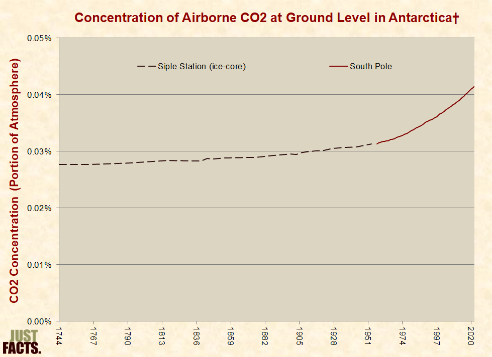
* Since the outset of the Industrial Revolution in the late 1700s,[59] the portion of the earth’s atmosphere that is comprised of carbon dioxide has increased from 0.028% to 0.041%, or by about 49%:
 |
* Per a 1971 article in the journal Science coauthored by climatologist Stephen Schneider, who later created the journal Climatic Change and was a founding member of the UN’s Intergovernmental Panel on Climate Change:[66]
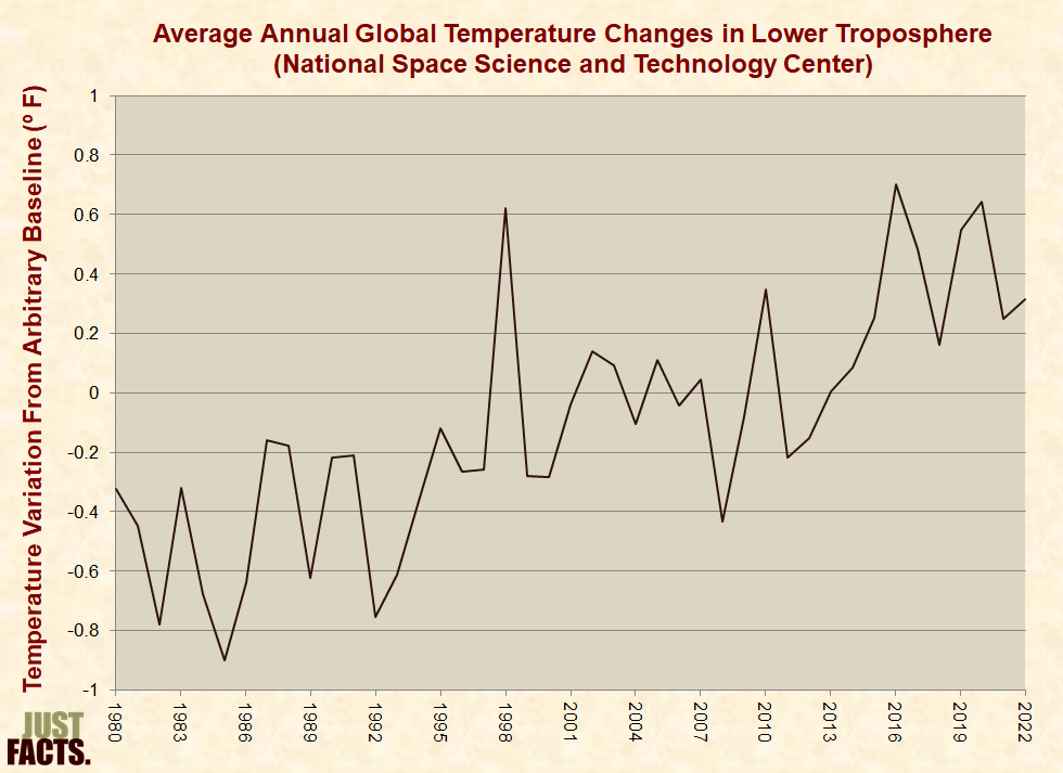
* Instruments located on satellites can measure certain properties of oxygen that vary with temperature. Data from these instruments is used to calculate the average temperatures of different layers of the Earth’s atmosphere.[68] [69]
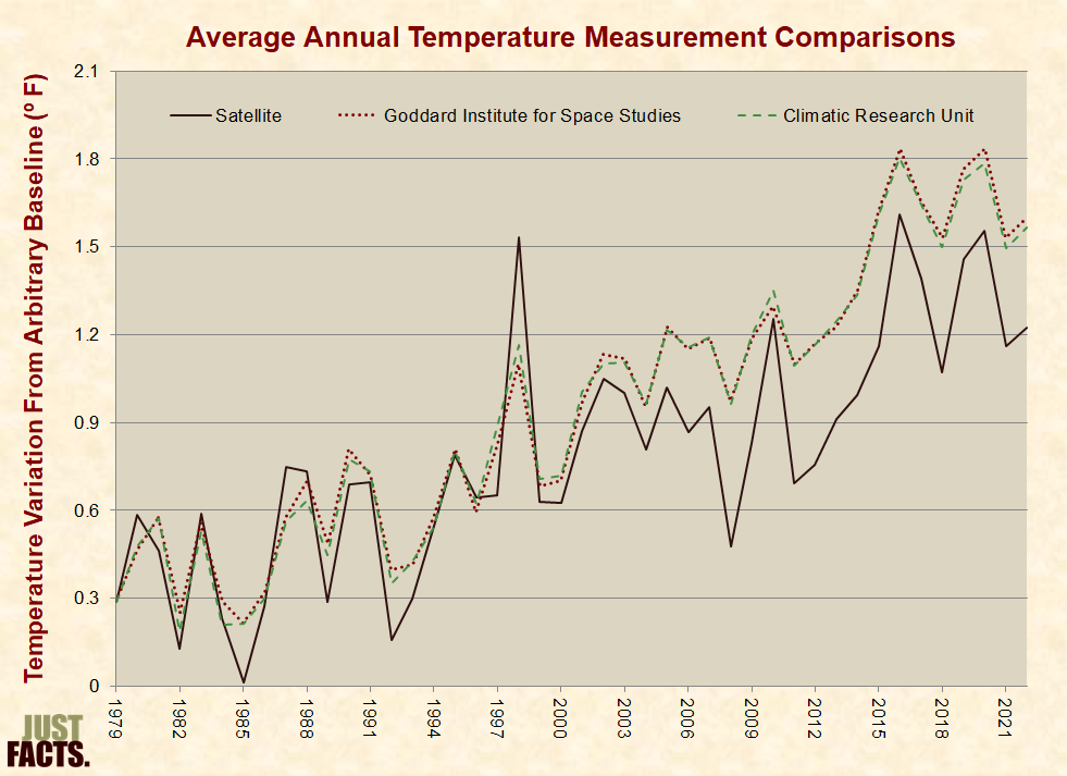
* The lowermost layer of the atmosphere, which is called the “lower troposphere,” ranges from ground level to about five miles (8 km) high.[70] [71] According to satellite data correlated and adjusted by the National Space Science and Technology Center at the University of Alabama Huntsville, the average temperature of the lower troposphere increased by 0.8ºF (0.5ºC) between the 1980s and the most-recent decade from 2013 to 2022:
* For reference, a temperature analysis of a borehole drilled on a glacier in Greenland found that the location was about 22ºF (12ºC) colder during the last ice age than it is now.[75]
* Sources of uncertainty in satellite-derived temperatures involve variations in satellite orbits, variations in measuring instruments, and variations in the calculations used to translate raw data into temperatures.[76] [77]
* A 2011 paper in the International Journal of Remote Sensing estimates that the accuracy of satellite-derived temperatures for the lower troposphere is “approaching” ±0.05ºF (0.03ºC) per decade, or ±0.18ºF (0.1ºC) over 30+ years.[78]
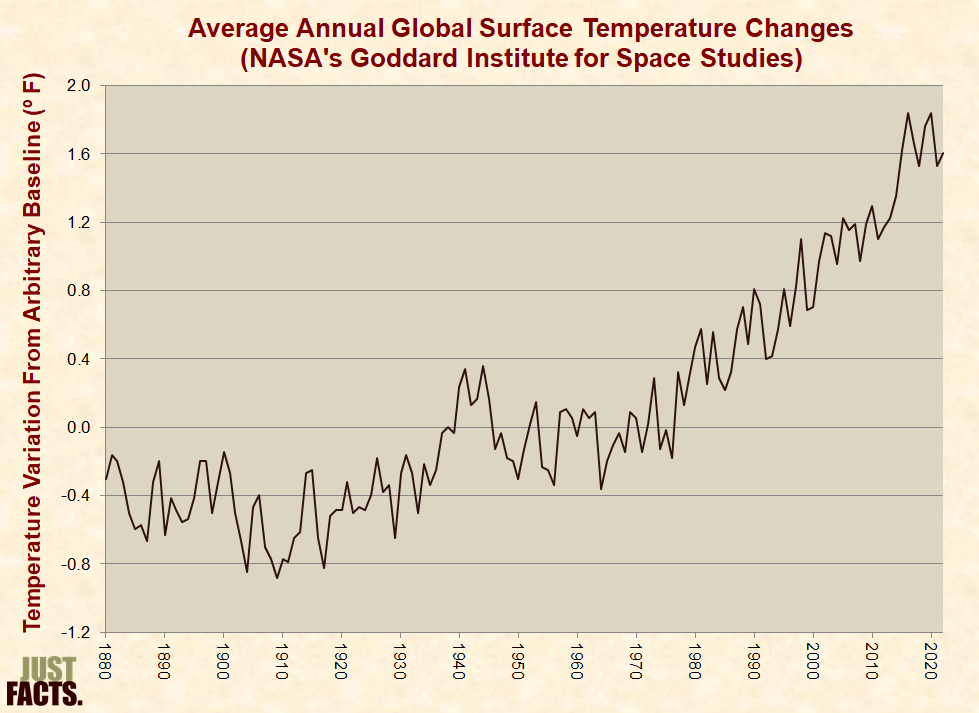
* According to temperature measurements taken near the Earth’s surface that are correlated and adjusted by NASA’s Goddard Institute for Space Studies, the Earth’s average temperature warmed by 1.6ºF (0.9ºC) between the 1880s and the most-recent decade from 2013 to 2022:
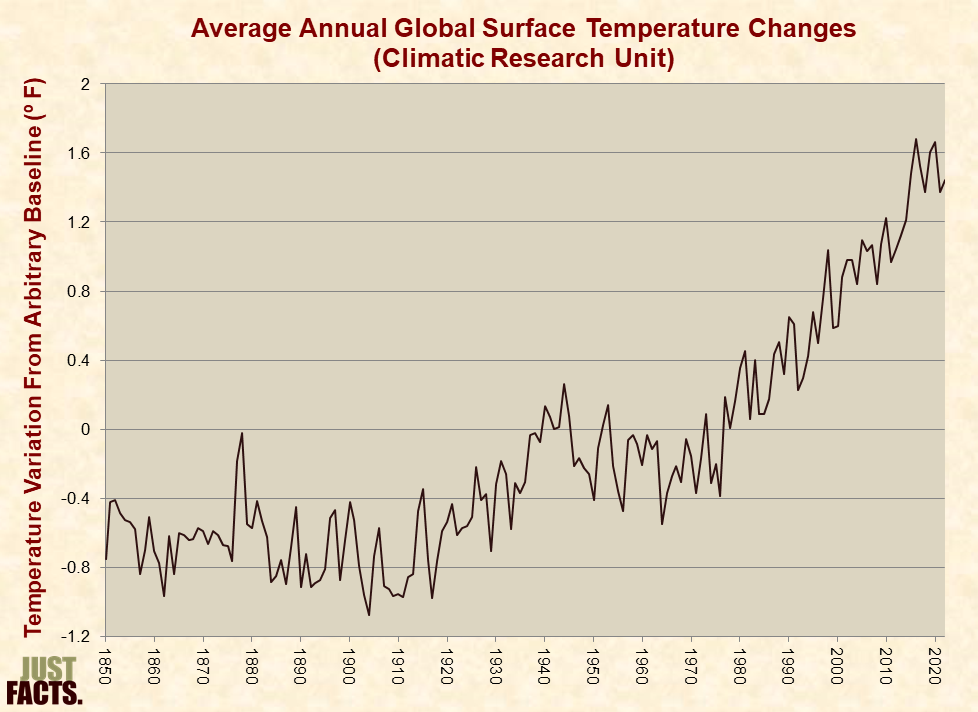
* According to temperature measurements taken near the Earth’s surface that are correlated and adjusted by the Climatic Research Unit of the University of East Anglia in the U.K., the Earth’s average temperature warmed by 2.0ºF (1.1ºC) between the 1850s and the most-recent decade from 2013 to 2022:
* Sources of uncertainty in surface temperature data include:
* A 2006 paper in the Journal of Geophysical Research that calculates uncertainties in surface temperature data states that a:
* Oceans constitute about 71% of the Earth’s surface.[98] Changes in air temperature over the world’s oceans are typically based on measurements of water temperature at depths varying from less than 3 feet to more than 49 feet.[99] [100] This data is combined with changes in air temperature over land areas to produce global averages.[101] [102]
* A 2001 paper in Geophysical Research Letters contrasted water and air temperature changes in the tropical Pacific Ocean using three sources of measurements. One of these was a series of buoys, each containing thermometers located ten feet above the water and at one foot below the water. The study found that water temperatures increased on average by 0.23ºF (0.13ºC) per decade between 1979 and 1999, while air temperatures cooled by 0.02 to 0.09ºF (0.01 to 0.06ºC) per decade during the same period.[103]
* A 2011 paper in the Journal of Geophysical Research examined the locations of 1,007 of the 1,221 monitoring stations used to determine average surface temperature changes across the continental United States. The paper found that 92% of these stations are positioned in sites that can cause errors of 1.8ºF (1ºC) or more.[104] [105] For example, some stations are located over asphalt (making them hotter at certain times), and others are located in partial shade (making them cooler at certain times). By comparing data from poorly positioned stations with other stations that are properly positioned, the study determined that the temperature irregularities in the poorly positioned stations cancel one another so that their average temperature trends are “statistically indistinguishable” from the properly positioned stations. As of May 2023, Just Facts is not aware of a similar study that has been conducted on a global basis.[106]
* From 1979 to 2022, the three temperature datasets posted above differed from one another by an annual average of 0.14ºF (0.08ºC). The largest gap between any of the datasets in any year was 0.49ºF (0.27ºC), and the smallest gap was 0º:
* A scientific, nationally representative survey commissioned in 2019 by Just Facts found that 34% of voters believe the earth has not become measurably warmer since the 1980s.[108] [109] [110]
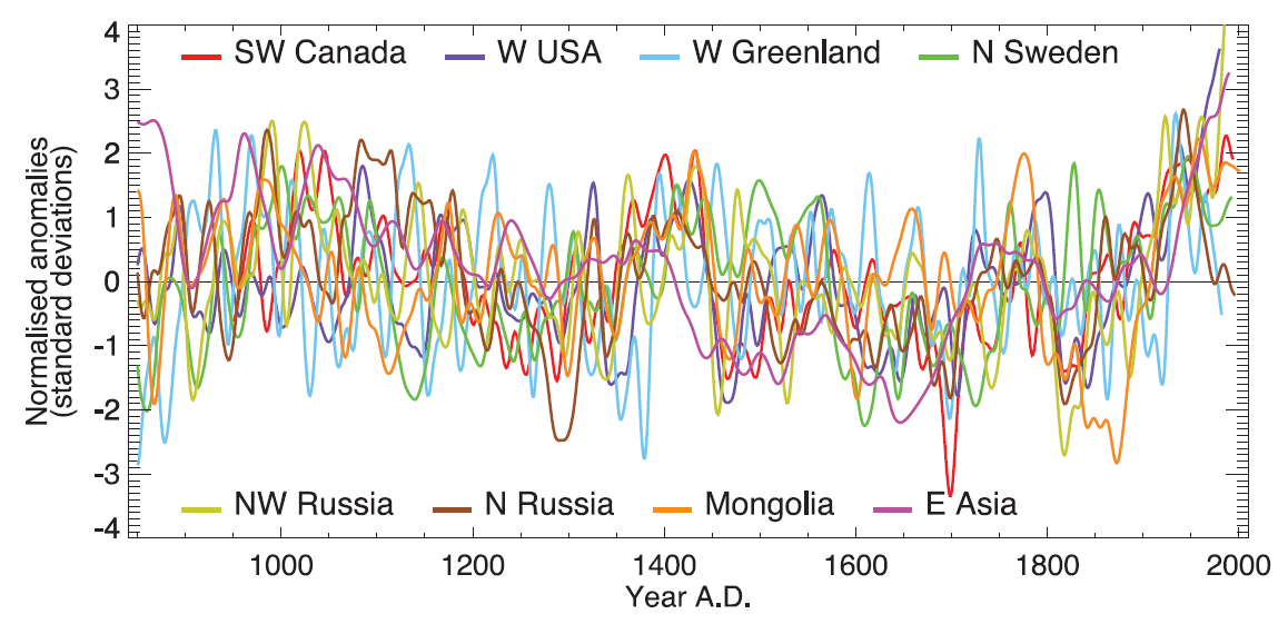
* To reconstruct global average temperatures in the era before instrumental measurements were made on a global scale, scientists use proxies that respond to changes in climate, such as the widths of tree rings and certain elements of the geological record, to estimate temperature variations in the past.[111] [112]
* The Intergovernmental Panel on Climate Change (IPCC) is a scientific body established in 1988 by the United Nations and World Meteorological Organization. It is the “leading international body for the assessment of climate change,” and its “work serves as the key basis for climate policy decisions made by governments throughout the world….”[113] [114] [115] The IPCC states:
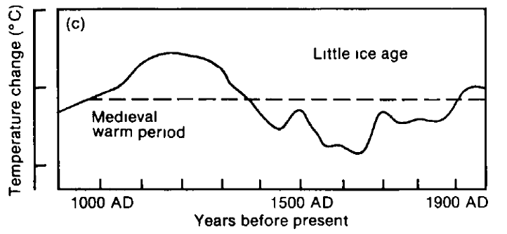
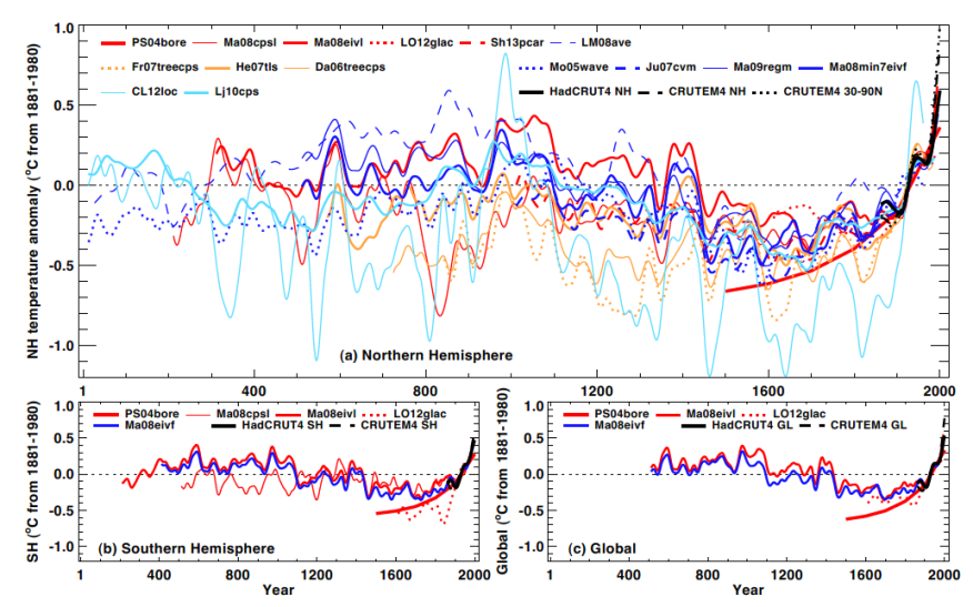
* The first IPCC report (1990) contains the following graph of average global temperature changes over the past 1,000 years based upon proxies. It shows a “Medieval warm period” that was warmer than the present era and a “Little Ice Age” that was cooler. The report states that:
* The second IPCC report (1995) states that “data prior to 1400 are too sparse to allow the reliable estimation of global mean temperature” and shows a graph of proxy-derived temperatures for Earth’s Northern Hemisphere from 1400 onward. This graph shows different details but a similar overall trend to the first report.[118]
* The third IPCC report (2001) states that the latest proxy studies indicate “the conventional terms of ‘Little Ice Age’ and ‘Medieval Warm Period’ appear to have limited utility in describing … global mean temperature changes in past centuries.” The report contains the following graph of average temperature changes in Earth’s Northern Hemisphere, showing higher temperatures at present than at any time in the past 1,000 years.

* This graph is called the “hockey stick graph” because the curve looks like a hockey stick laid on its side (click on the footnote for a graphic illustration).[120] The red part of the curve represents modern instrument-measured surface temperatures, the blue represents proxy data, the black line is a smoothed average of the proxy data, and the gray represents the margin of error with 95% confidence.[121] [122]
* The IPCC’s hockey stick graph was adapted from a 1999 paper in Geophysical Research Letters authored by climatologist Michael Mann and others. This paper was based upon a 1998 paper by the same authors that appeared in the journal Nature.[123] [124] Multiple versions of this graph appear in different sections of the IPCC report, including the “Scientific” section,[125] “Synthesis,”[126] and twice in the “Summary for Policymakers.”[127]
* This graph has been the subject of disputes in scientific journals,[128] [129] congressional hearings,[130] [131] a whistleblower document release,[132] and legal proceedings including a Freedom of Information Act lawsuit.[133] [134] These revealed the following facts:
* The fourth IPCC report (2007) states that “there are far from sufficient data to make any meaningful estimates of global medieval warmth,” and it shows the following graph of temperature changes for the Northern Hemisphere over the past 1,300 years. This graph, which is called a “spaghetti graph,” is constructed with data from 12 proxy studies spliced with instrument-measured surface temperatures (the dark black line on the right):

* The fourth IPCC report also presents a graph of proxy studies that does not splice in instrument-measured surface temperatures. It displays the following data from three proxy studies to show “the wide spread of values exhibited by the individual records that have been used to reconstruct” temperatures in the Northern Hemisphere:
* The fifth IPCC report (2013) states that challenges persist in reconstructing temperatures before the time of the instrumental record “due to limitations of spatial sampling, uncertainties in individual proxy records and challenges associated with the statistical methods used to calibrate and integrate multi-proxy information.” This report contains the following spaghetti graphs of proxy studies spliced with instrument-measured surface temperatures (the black lines):
* The sixth IPCC report (2021):
* The following are sources of uncertainty in proxy-derived temperatures:
* In 2009, an unknown individual(s) released more than 1,000 emails (many dealing with proxy studies) from the University of East Anglia’s Climatic Research Unit (CRU). The materials were authored by some of the world’s leading climate scientists and accompanied by the following note:
* These emails (commonly referred to as the ClimateGate emails) show IPCC scientists and authors:
* A 2001 ClimateGate email states:
* The continental United States contains 1.6% of the world’s surface area, and the entire United States (including Alaska and Hawaii) contains 1.9%.[182]
* A 2021 paper in the journal Atmosphere found that from 1979 through 2018, average temperatures in Antarctica have:
* A 2008 survey of 660 Virginia residents found that the most common answer people give for believing or disbelieving in global warming is their personal experience of the climate.[184]
* The state of Virginia contains 0.02% of the world’s surface area.[185]
* A 2008 paper in the Journal of Geophysical Research found that the area covered by sea ice in the Arctic was declining by about 4.0% per decade, while the area covered by sea ice in the Antarctic was increasing by about 1.7% per decade.[186] [187]
* In 2007, the New York Times published a story by Andrew Revkin entitled: “Scientists Report Severe Retreat of Arctic Ice.” The last paragraph of the story reads: “Sea ice around Antarctica has seen unusual winter expansions recently, and this week is near a record high.”[188]
* A 2006 paper in the Journal of Climate found that glaciers in the western Himalayan mountains thickened and expanded during 1961–2000, while glaciers in the eastern Himalayas decayed and retreated.[189]
* A 2006 paper in Geophysical Research Letters found that since 1979, Antarctica has been growing colder in the summer and fall seasons but warmer in the winter and spring seasons, except for 50% of East Antarctica, which has also been cooling in the winter.[190]
North Pole
* In 2000, James J. McCarthy, a Harvard oceanographer and IPCC co-chair,[191] saw a mile-wide stretch of open ocean at the North Pole while serving as a guest lecturer on an Arctic tourist cruise. He then informed the New York Times, which ran a front-page story claiming:
* Like the New York Times:
* Two days after the New York Times article was published, the London Times quoted a professor of ocean physics at Cambridge who stated, “Claims that the North Pole is now ice-free for the first time in 50 million years [are] complete rubbish, absolute nonsense.”[195] [196]
* Eight days later, the New York Times issued a correction stating that:
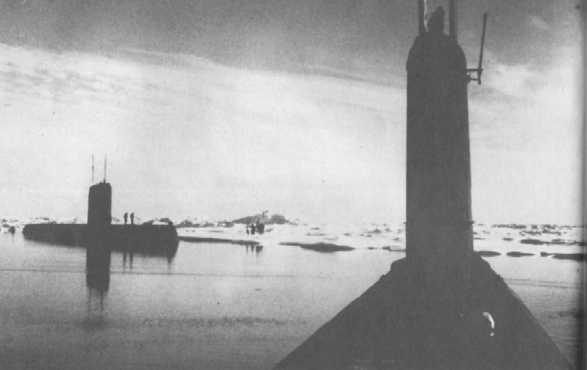
* In the June 13, 1963 issue of New Scientist, a U.S. Navy sonar specialist and onboard scientist for several submarine missions to the Artic and North Pole, described the ice conditions by stating:
* This picture shows two U.S. submarines surfacing at the North Pole in August of 1962:
* In 2013, “Forecast the Facts”—a “grassroots human rights organization dedicated to ensuring that Americans hear the truth about climate change”—published the following graphic purporting to show a recent photo of the North Pole:
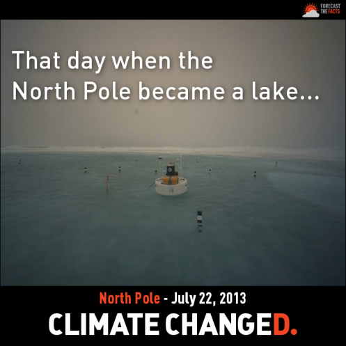
* Along with the graphic, Forecast the Facts claimed that this “lake formed at the North Pole due to unprecedented melting Arctic sea ice.”[206] [207]
* The photo above was not taken at the North Pole. It was taken from a buoy located about 350 miles from the North Pole.[208] [209] [210] [211] [212]
* The first humans to visit the surface of the North Pole region during summer were the crew of the USS Skate, a nuclear submarine that surfaced 40 miles from the North Pole in August of 1958.[213] In the January 1959 issue of Life magazine, the commander of this mission described the ice cover by stating:
* Within four days after Forecast the Facts published the graphic above, media outlets made the following claims:
* None of these articles stated or implied that such conditions have prevailed for as long as mankind has had the technology to visit the surface of the North Pole in the summer.[225] [226]
* After publishing an article documenting the facts above, Just Facts contacted Forecast the Facts to offer an opportunity to respond.[227] As of May 2023, Forecast the Facts has not replied or issued a correction.[228] [229]
* Forecast the Facts later changed its name to “ClimateTruth.org.”[230] Its board of academic advisors included:
* In a 2017 television appearance, Bill Nye, the celebrity “Science Guy” asserted that without human activity, the climate would currently “look like it did in 1750,” and “you could not grow wine-worthy grapes in Britain, as you can today, because the climate is changing.”[232]
* Archaeological and historical records show that wine grapes were grown in England from about 1000–1400 AD, as documented in the following books:
* The Intergovernmental Panel on Climate Change (IPCC) has recognized that “multiple strands” of historical and archeological evidence show “a period of widespread and generally warmer temperatures” in Western Europe during the Middle Ages. However, the IPCC concludes that “in medieval times, as now, climate was unlikely to have changed in the same direction, or by the same magnitude, everywhere.” Some examples of what this evidence shows include the following:
* In addition to carbon dioxide emissions from human usage of fossil fuels, other factors that have been implicated by scientists as causes of modern climate change include but are not limited to:
* The natural variability of Earth’s climate is such that:
* A central debate among scientists about man-made greenhouse gases involves how much natural processes reduce or amplify the effects of these gases. Positive feedbacks amplify the effects, and negative feedbacks diminish them.[252]
* A 2006 paper in the Journal of Climate states that the feedbacks used in climate models are based upon “methods that … do not allow any observational assessment” because many variables are involved, and “it is not possible … to insure that only one variable is changing.”[253]
* The climate models included in the 2007 IPCC report were programmed with positive feedbacks for water vapor that more than double the warming effect of CO2.[254] This is based upon the fact that warmer air evaporates more water, thus creating more water vapor, which is a greenhouse gas.[255] [256]
* A 2009 paper in the journal Theoretical and Applied Climatology found that during 1973–2007, humidity increased in the lowest part of Earth’s atmosphere but decreased at higher altitudes, implying that the “long-term water vapor feedback is negative—that it would reduce rather than amplify” the warming effect of CO2. A caveat of this finding is that it is based upon weather balloon data, which “must be treated with great caution, particularly at [higher] altitudes….”[257] [258]
* The climate models included in the 2007 IPCC report were programmed with positive feedbacks for clouds that amplify the warming effect of CO2 by 10%–50%.[259]
* A 2006 paper in the Journal of Climate states that the “sign and the magnitude of the global mean cloud feedback depends on so many factors that it remains very uncertain.” This is because some types of clouds trap heat while others reflect it.[260] [261] [262]
* A 2007 paper in Geophysical Research Letters found that ice clouds (also called cirrus clouds)[263] exert a “strongly negative” feedback to temperature changes, regardless of whether these changes are increases or decreases. A caveat of this finding is that the feedback process operates “on a time scale of weeks,” and “it is not obvious whether similar behavior would occur on the longer time scales associated with global warming.”[264] [265]
* In a 1989 article in the EPA Journal, Sandra Postel, the vice president for research at Worldwatch Institute claimed:
* Based on three long-term satellite datasets, a paper published by the journal Nature Climate Change in 2016 found “a persistent and widespread increase” in greening “over 25% to 50% of the global vegetated area” from 1982 to 2014, “whereas less than 4% of the globe” had less greening over this period. Using “ten global ecosystem models,” the authors estimated that “70% of the observed greening trend” was due to more CO2 in the air.[267] [268]
* In 2018, the journal Nature published a study that:
* Per the Journal of Climate, other feedbacks that may have “a substantial impact on the magnitude, the pattern, or the timing of climate warming” include snow coverage, temperature gradients in Earth’s atmosphere, aerosols, trace gases, soil moisture changes, and ocean processes.[270]
* In 1989, climatologist Stephen Schneider—the creator of the journal Climatic Change and one of the founding members of the UN’s Intergovernmental Panel on Climate Change—told Discover magazine that in order to “reduce the risk of potentially disastrous climate change”:
* In 1988, Dr. James Hansen, a “world-renowned climatologist” and Director of NASA’s Goddard Institute for Space Studies (GISS),[273] [274] predicted that the average global temperature would increase by about 1.8ºF between the 1980s and 2010s.[275] In reality, it increased by 0.7ºF between these decades,[276] or by two-fifths of his projection.[277]
* In 1989, Dr. David Rind, an atmospheric scientist at the Goddard Institute for Space Studies and a “leading researcher” on global warming, wrote that his agency’s “model’s forecast for the next 50 years” predicts an average global temperature increase of “3.6ºF by the year 2020.”[278] [279] In reality, it increased by about 0.7ºF between the 1980s and the decade that ended in 2020,[280] or by one-fifth of his projection.[281]
* In 1989, Dr. Noel Brown, an environmental diplomat and Director of the United Nations Environment Program,[282] [283] [284] predicted that the average global temperature “will rise 1 to 7 degrees in the next 30 years.”[285] [286] In reality, it increased by about 0.7ºF between the 1980s and the 2010s,[287] or by seven-tenths to one-tenth of his projection.[288]
* In 1989, William H. Mansfield III, the deputy executive director of the United Nations Environment Programme, wrote that “global warming may be the greatest challenge facing humankind,” and “any change of temperature, rainfall, and sea level of the magnitude now anticipated will be destructive to natural systems” like “plant” life.[289]
* A 2003 paper in the journal Science found that a principal measure of worldwide vegetation productivity increased by 6.2% between 1982 and 1999. The paper notes that this occurred during a period in which human population increased by 37%, the level of atmospheric CO2 increased by 9%, and the Earth “had two of the warmest decades in the instrumental record.”[290] [291]
* A 2004 paper in the journal BioScience attributes the rising vegetation productivity found in the 2003 Science paper to “higher temperatures, longer temperate growing seasons, more rainfall in some previously water-limited areas,” and more sunlight. The following map shows these productivity changes, with green signifying higher vegetation productivity and red lower:
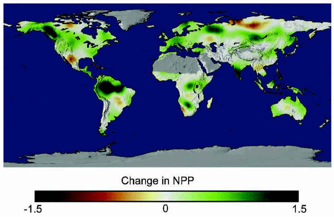
(Reproduced with permission of the University of California Press)
* Based on projections published by the journal PLOS Biology, Time magazine claimed in 2015:
* A paper published by the journal Nature Climate Change in 2016 analyzed three long-term satellite datasets and found “a persistent and widespread increase” in “greening” or plant growth “over 25% to 50% of the global vegetated area” from 1982 to 2014, “whereas less than 4% of the globe” had less greening over this period. Using “ten global ecosystem models,” the authors estimated that “70% of the observed greening trend” was due to more CO2 in the air.[295] [296]
* As of 2022, the concentration of CO2 in Earth’s atmosphere is about 415 parts per million (ppm).[297] Per an academic text that discusses increasing the productivity of commercial greenhouses:
* In 1989, William H. Mansfield III, the deputy executive director of the United Nations (UN) Environment Programme, wrote that “forests would be adversely affected” by global warming.[299]
* Per reports published by the (UN) Food and Agriculture Organization from 2018 through 2022:
* “Tree cover” is a measure of greenery that includes forests plus land covered by trees in:
* In 2018, the journal Nature published a study that:
* In 1989, Sandra Henderson, a biogeographer at EPA’s Environmental Research Laboratory, wrote in the EPA Journal that:
* Roughly 1.2 million species have been cataloged.[309] A loss of 20% of these would be 240,000 species.[310]
* In and around the period covered by Henderson’s projections:
* For more facts about the extinction rates of land and sea creatures, read Just Facts’ article, “Is Ocean Life on the Brink of Mass Extinction?”
* In 1975, Newsweek claimed that the world was “cooling” and:
* Per a 2003 report by the United Nations Food and Agriculture Organization, between the mid-1970s and late 1990s, food consumption per person increased by 15% worldwide, 25% in developing countries, and more than 36% in China. During this same period:
* Three decades after it reported that global cooling would reduce food production, Newsweek claimed:
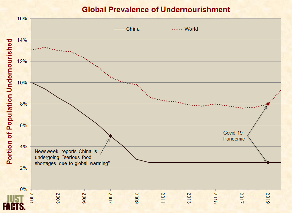
* From 2001 to 2020, the portion of the population in China that was undernourished decreased from 10% to 2.5%, and the portion of the world population that was undernourished decreased from 13% to 9%:
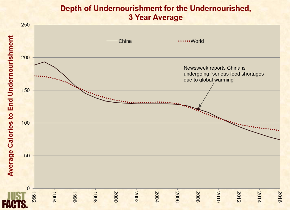
* From 1992 to 2016, the average number of daily calories needed to lift undernourished people in China out of that condition decreased from 188 to 74 calories per person. In the same period, the average for all the undernourished people of the world decreased from 172 to 88 calories:
* In 1989, William H. Mansfield III, the deputy executive director of the United Nations Environment Programme, wrote that “concern about climate change impacts has sent storm warning flags aloft in the United Nations” because global warming would “disrupt agriculture” and “adversely” affect “food supplies.”[325]
* In 2017, the United Nations reported:
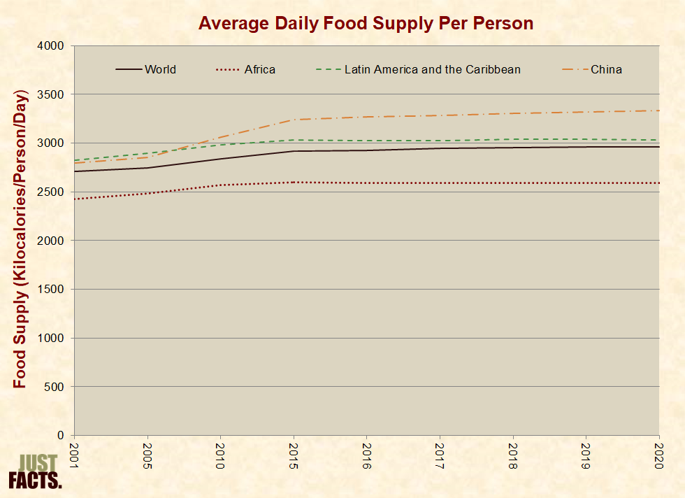
* From 2000 to 2021, global average daily food supply per person increased by 9%, with gains of 7% in Africa, 19% in China, and 8% in Latin America and the Caribbean:
* Increased ocean temperatures cause average sea levels to rise because water expands as it becomes warmer. Per a 2006 paper in the journal Nature, this thermal expansion is calculated to have the largest current influence on average sea level changes. The second largest influence is calculated to be the melting of glaciers and mountain icecaps.[328] Per a 2010 paper in Geophysical Research Letters, melting sea ice is responsible for less than 2% of current sea level changes.[329] [330]
* Sea level is not evenly distributed across the world like it is in small bodies of water like lakes. For instance, the sea level in the Indian Ocean is about 330 feet below the worldwide average, while the sea level in Ireland is about 200 feet above the average. Such variations are caused by gravity, winds, and currents, and the effects of these phenomena are dynamic. For example:
* Scientists have estimated sea levels going back to the year 1700 using data from local tide gauges. These instruments measure the level of the sea relative to reference points on land. Per the Sea Level Research Group at the University of Colorado, “Although the global network of tide gauges comprises of a poorly distributed sea level measurement system, it offers the only source of historical, precise, long-term sea level data.”[333] [334]
* According to tide gauge data, the average global sea level has been generally rising since 1860 or earlier. This is about 45 years before surface temperatures began to rise and 96 years before man-made emissions of CO2 reached 1% of natural emissions.[335] [336] [337]
* According to tide gauge data, the average worldwide sea level rose by about 7 inches (18 cm) during the 20th century. A 2022 report by the Intergovernmental Panel on Climate Change uses certain models that project an acceleration of this trend. These models predict sea level increases ranging from 17 to 33 inches (43–84 cm) from 1986–2005 to 2100.[338] [339] [340]
* Using tide gauge data, a 2006 paper in Geophysical Research Letters found:
* Using updated tide gauge data from two earlier studies (including the 2006 study cited above), a 2011 paper in the Journal of Coastal Research found “small decelerations” in global average sea level rises during the 20th century, which is “consistent with a number of earlier studies of worldwide-gauge records.”[342]
* Since late 1992, instruments on satellites have been collecting data that scientists use to calculate the mean global sea level.[343] [344] Averaging the eight available datasets, the global mean sea level increased by 2.0 inches (50 mm) between the 1990s and the recent decade from 2011 to 2020:
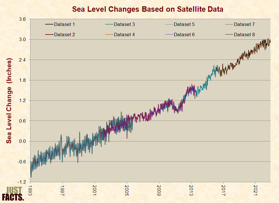
* Click here for an article from Just Facts that exposes how certain scientists and media outlets have misled the public about sea level acceleration.
* Coral reef islands are considered to be highly vulnerable to rising oceans because they sit slightly above sea level and are made of loosely bound sediments. These islands are typically located in the Pacific Ocean and are mainly comprised of gravel, silt, and sand that has accumulated on coral reefs. The habitable land of some nations, such as Tuvalu, Kiribati and the Maldives, consists almost entirely of coral reef islands.
* At the 2009 United Nations Climate Summit in Copenhagen, Denmark, Ian Fry of the government of Tuvalu addressed the conference and claimed:
* In 2018, the journal Nature Communications published the “first comprehensive national-scale analysis” of Tuvalu’s land resources. The analysis found that the nation’s total land area increased by 2.9% from 1971 to 2014.[349]
* The authors of a 2010 paper in the journal Global and Planetary Change used aerial and satellite photographs to conduct “the first quantitative analysis of physical changes” in 27 central Pacific coral reef islands over a 19- to 61-year period. They found that:
* Click here for an article and video from Just Facts about how a media outlet misled the public about the effect of sea-level rise on the Pacific island nation of Kiribati.
* In 1989, the Associated Press reported: “A senior U.N. environmental official says entire nations could be wiped off the face of the Earth by rising sea levels if the global warming trend is not reversed by the year 2000. Coastal flooding and crop failures would create an exodus of ‘eco-refugees,’ threatening political chaos, said Noel Brown, director of the New York office of the U.N. Environment Program.”[351]
* In 1989, William H. Mansfield III, the deputy executive director of the United Nations Environment Programme, wrote:
* A study of satellite data published by the journal Nature Climate Change in 2016 found that from 1985 to 2015:
* In his 1992 book, Earth in the Balance, Democratic U.S. Senator Al Gore claimed:
* In 2008, scientists with the Center for Environment and Geographic Information Services in Bangladesh announced that their study of satellite images and maps shows that Bangladesh gained about 1,000 square kilometers of land since 1973.[357] [358] [359]
* From 1993 to 2023, the population of Bangladesh increased from 119 million to 167 million people, or by 40%.[360]
* From 1990 to 2021, the coastal population of Florida increased from 10.1 million to 16.3 million people, or by 61%.[361] [362]
* An Inconvenient Truth is an Academy Award-winning documentary about Al Gore’s “commitment to expose the myths and misconceptions that surround global warming and inspire actions to prevent it.”[363] In this 2006 film, Gore shows the following computer simulation of what would happen to the shorelines of Florida and the San Francisco Bay if sea levels were to rise by twenty feet, while providing no timeframe for such an event to occur:
* A 20-foot rise in sea level equals 8 to 34 times the full range of 110-year projections for sea level rise in the 2007 report by the Intergovernmental Panel on Climate Change.[365]
* In a 1995 article about global warming and rising sea levels, the New York Times reported:
* A 1996 travel guide titled Best Beach Vacations in the Mid-Atlantic: From New York to Washington, D.C. featured 95 beaches.[367] All of these beaches still exist 27 years later in 2023:[368]
* The first 100 results for a 2023 Google search for East Coast beaches gone didn’t reveal any beaches that have disappeared.[370]
* A “tropical cyclone” is a circular wind and low-pressure system that develops over warm oceans in the tropics. Cyclones with winds ranging from 39 to 73 miles per hour are called “tropical storms,” and those with winds exceeding 73 miles per hour are called “hurricanes.” Technically, there are different names for cyclones with hurricane-force winds in different areas of the world, but for the sake of simplicity, this research refers to them as hurricanes.[371] [372]
* In 2004, James McCarthy, a professor of biological oceanography at Harvard University, claimed: “As the world warms, we expect more and more intense tropical hurricanes and cyclones.”[373]
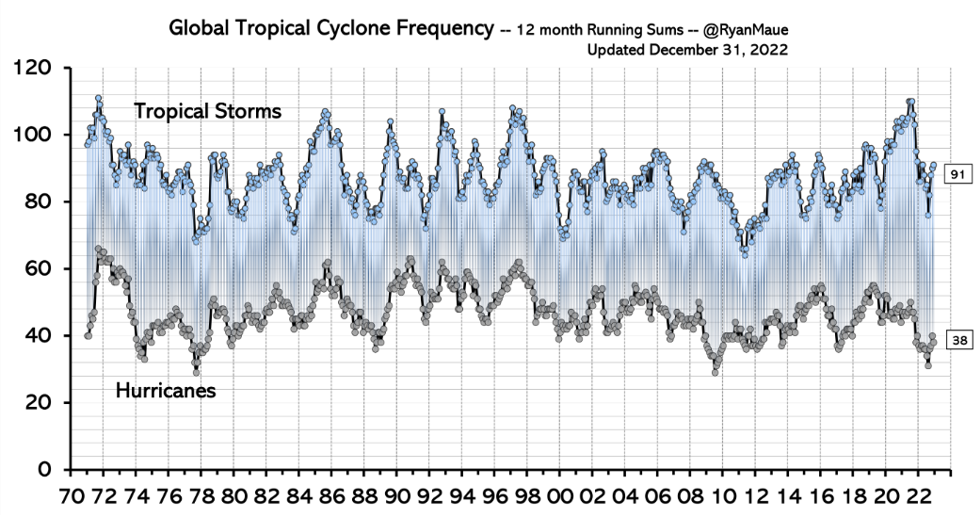
* Since 1970, the annual frequencies of tropical storms and hurricanes have varied as follows:
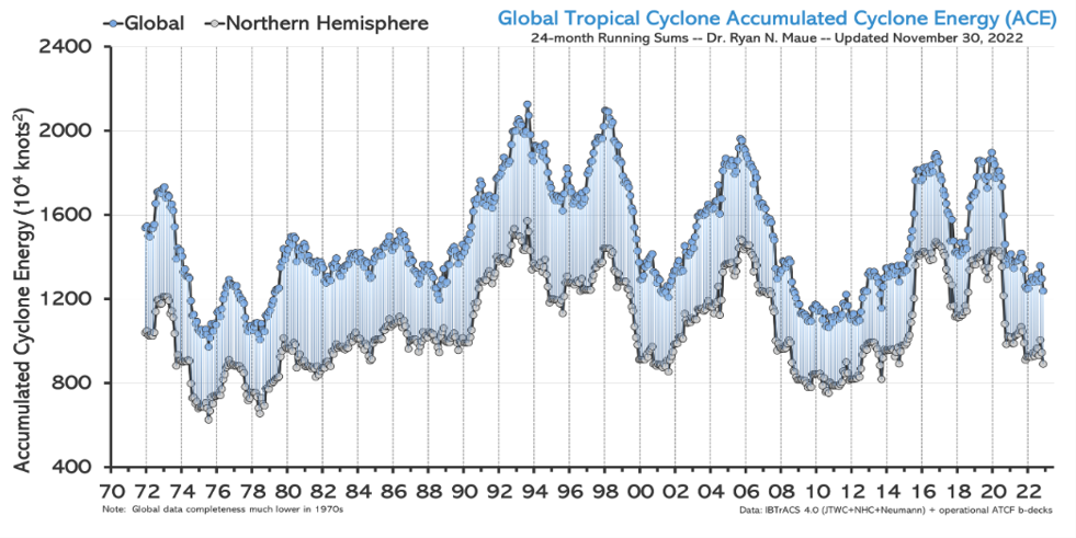
* “Accumulated cyclone energy” is an index that “approximates the collective intensity and duration of tropical storms and hurricanes….”[375] Since 1970, the accumulated cyclone energies of tropical storms and hurricanes have varied as follows:
* A scientific, nationally representative survey commissioned in 2019 by Just Facts found that 64% of voters believe the number and intensity of hurricanes and tropical storms have generally increased since the 1980s.[377] [378] [379]
* Click here for an article from Just Facts about how media outlets have misled the public about trends in hurricanes and rainfall.
* In 1989, Dr. David Rind, an atmospheric scientist at the Goddard Institute for Space Studies predicted that “rainfall patterns would likely be substantially altered” from global warming “by the year 2020.” He claimed that these changes would create the “threat of large-scale disruptions of agricultural and economic productivity, and water shortages in some areas.”[380]
* In 2017, Politico published an article by meteorologist Eric Holthaus claiming that “climate change is making rainstorms everywhere worse, but particularly on the Gulf Coast.”[381] As proof of this, he links to an article in the London Guardian by Professor John Abraham, who claims: “In the United States, there has been a marked increase in the most intense rainfall events across the country. This has resulted in more severe flooding throughout the country.”[382] [383]
* A 2011 paper in the Hydrological Sciences Journal examined rainfall-related U.S. flood trends from 200 water gauges with records extending from 85 to 127 years ago and found:
* A study published in 2012 by the journal Nature examined drought trends over the past 60 years and found the following:
* In contradiction to the findings of prior studies that used “climate models” to study “changes in areas under droughts,” a 2013 paper in the journal Theoretical and Applied Climatology used global satellite observations and found “no significant trend in the areas under drought over land in the past three decades.” The study, however, found increasing drought over land in the Southern Hemisphere. With regard to this:
* In 2013, the Intergovernmental Panel on Climate Change (IPCC) reported:
* Regarding drought, the same 2013 IPCC report stated that previous claims of “global increasing trends in drought” were “probably overstated” and:
* A 2015 paper in the International Journal of Climatology studied extreme rainfall in England and Wales found that “contrary to previous results based on shorter periods, no significant trends of the most intense categories are found between 1931 and 2014.”[390]
* A 2015 paper in the Journal of Hydrology examined rainfall measurements “made at nearly 1,000 stations located in 114 countries” and:
* Per a 2022 paper in the journal Philosophical Transactions (the world’s first and longest-running scientific journal[392]):
* In 2011, Dr. Paul R. Epstein, a member of the IPCC and the associate director of the Center for Health and the Global Environment at Harvard Medical School, claimed that global warming was setting the stage for “even more punishing tornadoes.”[398] [399]
* In 2013, Michael Mann, a climatologist and the lead author of the IPCC’s hockey stick graph, predicted “greater frequency and intensity of tornadoes as a result of human-caused climate change.”[400] [401]
* In 2019, U.S. Senator Bernie Sanders claimed the “science is clear” that “climate change is making extreme weather events, including tornadoes, worse.”[402]
* Per the National Oceanic and Atmospheric Administration (NOAA):
* Since the 1950s, the frequency of strong-to-violent tornadoes in the U.S. have varied as follows:
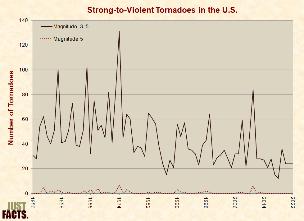
* A 2000 paper in the journal Weather and Forecasting studied economic damages from tornadoes in the U.S. during 1890–1999 and concluded:
* A 2013 paper in the journal Environmental Hazards estimated the normalized economic damages from tornadoes in the U.S. during 1950–2011 and found “a sharp decline in tornado damage.” Per the paper, “normalization provides an estimate of the damage that would occur if past events occurred under a common base year’s societal conditions.”[408]
* In 2010, Environment America, a federation of environmental organizations, published a report entitled “Global Warming and Extreme Weather: The Science, the Forecast, and the Impacts on America.” The report uses the word “death” (or synonyms for it) 18 times and claims:
* In 2011, Ph.D. biologist Richard Hilderman wrote an op-ed claiming:[410]
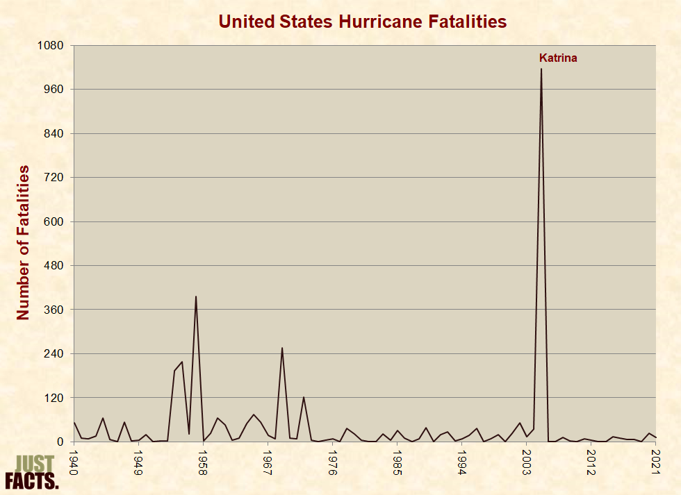
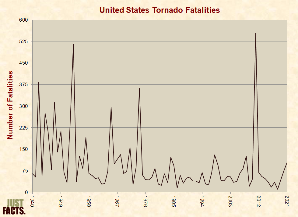
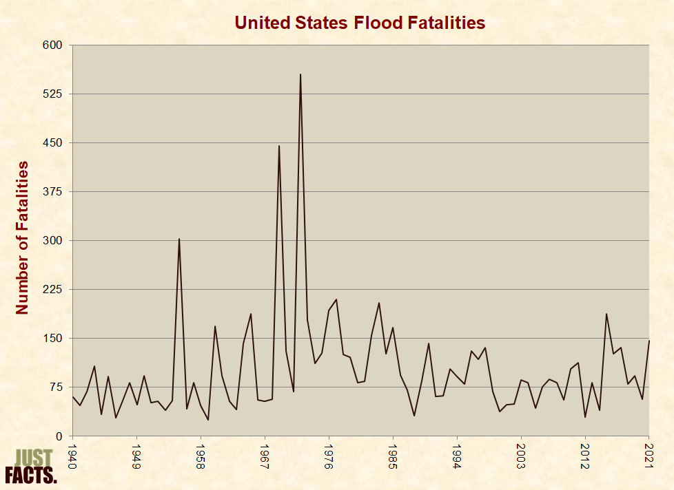
* The following graphs show the number of weather-related fatalities from various causes for as far back in time as the U.S. National Weather Service has records:
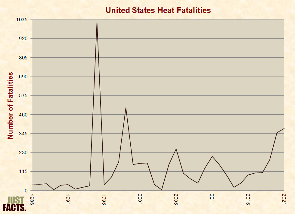
NOTE: Data on heat fatalities is subject to considerable uncertainty.[416]

NOTE: Data on cold fatalities is subject to considerable uncertainty.[418]
* Vector-borne diseases are illnesses that are usually transmitted by bloodsucking creatures like mosquitoes, ticks, and fleas.[419] [420]
* In 1989, William H. Mansfield III, the deputy executive director of the United Nations Environment Programme, wrote that global warming would harm “human health” and “could enlarge tropical climate bringing with it yellow fever, malaria, and other diseases.”[421]
* In 2017, Politico alleged:
* In 2012, The Lancet (a prestigious medical journal[423]) published research about vector-borne diseases that found the following:
* In 2016, the journal Nature Communications published a study about the effects of human activities on mosquito populations in North America over the past century. Based on three long-term datasets, the authors reported:
* Decades after DDT was restricted and banned in the U.S. and around the world, the World Health Organization and some environmental organizations have endorsed using DDT inside of homes to combat malaria.[441]
* Per a 2000 paper in the British Medical Journal:
* The National Oceanic and Atmospheric Administration (NOAA) maintains a database of “weather and climate disasters since 1980 where overall damages/costs reached or exceeded $1 billion.”[443] Various environmental activists, scholars, and journalists have cited these data as evidence that global warming is causing economic damage, such as:
* NOAA’s database of billion-dollar-plus weather and climate disasters is adjusted for inflation but not for changes in population and economic development.[449] [450] [451]
* In 2008, the journal Natural Hazards published a paper that studied U.S. economic damages from hurricanes from 1900 to 2005 and found:
* In 2018, the journal Nature Sustainability published a paper that studied U.S. economic damages from hurricanes from 1900 to 2015 and found:
* Scientists and government officials have proposed and/or implemented the following actions to reduce greenhouse gases:
* The administrative body of the United Nations Framework Convention on Climate Change has stated:
* In 1997, an international body established by a treaty called the “United Nations Framework Convention on Climate Change” adopted an addition to this treaty called the Kyoto Protocol (so named because it was adopted in Kyoto, Japan). In 2005, this protocol became legally binding on the countries that ratified it. Its central provision requires 37 developed nations (such as Germany and Japan) to reduce their combined greenhouse gas emissions to about 5% below 1990 levels by no later than 2008–2012. The agreement:
* Before the Kyoto Protocol was adopted by the treaty conference, the United States Senate unanimously passed (by a vote of 95–0) a resolution stating that the U.S. should not be a party to any climate change agreement in Kyoto or thereafter that exempts developing nations from its provisions.[489] [490]
* The U.S. Constitution requires the approval of the president and a two-thirds majority vote of the Senate to ratify a treaty.[491]
* A year after the Kyoto Protocol was adopted by the treaty conference, President Bill Clinton approved the treaty, and his administration repeatedly stated that he would present the treaty to the Senate for ratification. He never did this.[492]
* In March 2001, fulfilling a campaign promise,[493] President George W. Bush announced that his administration would not pursue implementation of the Kyoto treaty.[494]
* With the exception of the United States, all the major developed nations ratified the Kyoto Protocol.[495]
* From 1990 to 2000, combined CO2 emissions in developed nations decreased by about 3%. This was primarily due to Russia, which underwent an economic collapse in 1990 that reduced their greenhouse gas emissions by about 40%. The other developed countries increased their combined emissions by about 8%.[496] [497]
* From 2008 (the beginning of the Kyoto Protocol’s compliance period[498]) to 2021, the combined annual CO2 emissions of the developed countries that ratified the treaty decreased by 13%. During the same period, annual U.S. emissions of CO2 decreased by 15%:

[499] [500] [501] [502] [503] [504]
* In the decade following the adoption of the Kyoto Protocol (1997–2007), Earth’s atmospheric CO2 concentration increased by 5.3% or 19 parts per million, which is 35% more than the increase in the decade before the treaty.[505]
* In 2011, Russia, Japan, and Canada announced they would not extend their participation in the Kyoto Protocol beyond 2012 because developing nations were exempted from its conditions.[506] In 2010, the head of the European Commission’s climate unit stated that the European Union’s participation in the Kyoto Protocol after 2012 will be based upon the participation of Russia and Japan.[507]
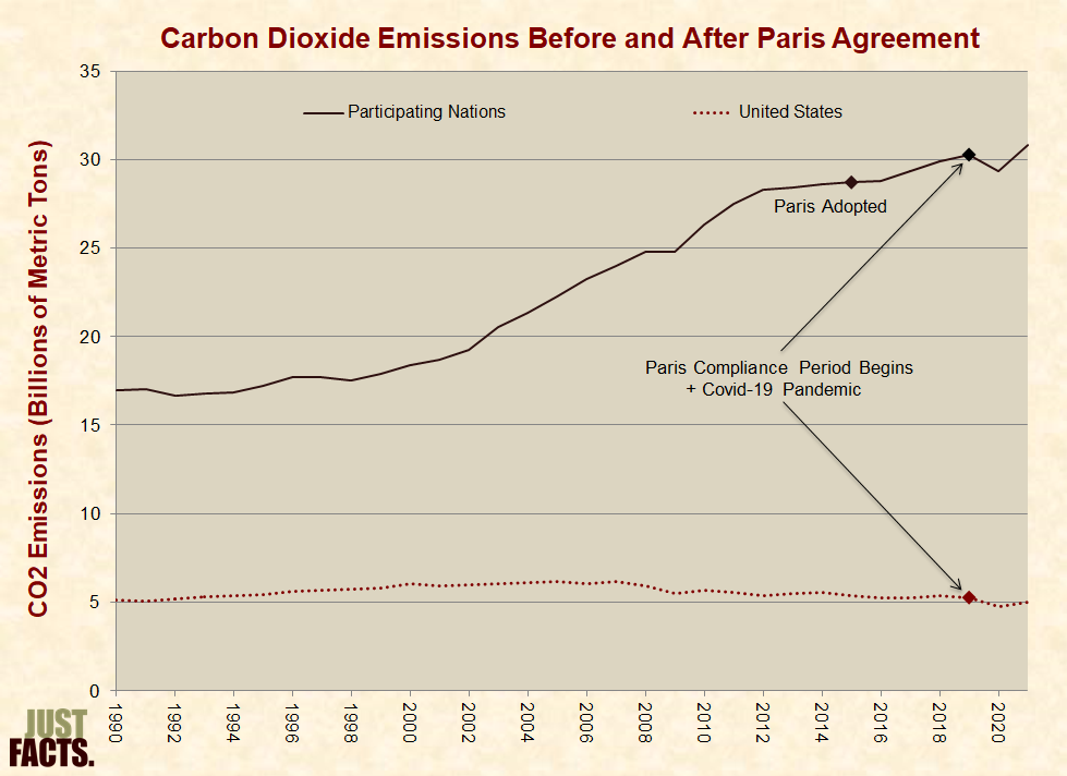
* In 2015, an international body established by a treaty called the United Nations Framework Convention on Climate Change adopted an accord called the Paris Agreement. Its primary aim “is to strengthen global response to the threat of climate change” by limiting the increase in global temperature to “well below 2 degrees Celsius [3.6° F] above pre-industrial levels.”[508] This agreement:
* The U.S. Constitution requires the approval of the president and a two-thirds majority vote of the Senate to ratify a treaty.[519]
* In August of 2016, Democratic President Barack Obama approved the Paris Agreement without submitting it to the Senate for approval.[520] [521] [522]
* In June of 2017, fulfilling a campaign promise,[523] [524] Republican President Donald Trump announced that he is withdrawing the U.S. from the Paris Agreement.[525] The withdrawal became official in November of 2020.[526]
* In January of 2021, on his first day in office, Democratic President Joe Biden announced that he is bringing the U.S. back into the Paris Agreement.[527] This re-entry became official one month later.[528]
* As of May 2023, 195 of 197 parties to the United Nations Framework Convention on Climate Change had ratified the Paris Agreement.[529] [530]
* The Paris Agreement’s compliance period began in 2020. From 2015 (the year the agreement was adopted[531]) to 2022, the combined annual CO2 emissions of the countries that ratified the treaty increased by 7%. During the same period, U.S. emissions of CO2 decreased by 7%.
* The Democratic Party Platform states:
* The Republican Party Platform states:
* In 2009, the U.S. House of Representatives passed a bill that would have capped most sources of greenhouse gas emissions in the U.S. at 17% below 2005 levels by 2020 and at 83% below 2005 levels by 2050.[539]
* This bill passed the House by a vote of 219–212, with 82% of Democrats voting for it and 94% of Republicans voting against it (click here for a record of how each Representative voted).[540] The bill was then forwarded to the Senate and never voted upon.[541]
* In 2009, the Obama administration EPA issued a finding that greenhouse gases “threaten the public health and welfare of current and future generations.” This finding allowed the administration to regulate greenhouse gases under the Clean Air Act.[542] [543]
* In 2010, 41 U.S. Senators sponsored a resolution that would have overturned the Obama administration’s authority to regulate greenhouse gases.[544] [545] A vote to advance the resolution failed 47 to 53, with all Republicans and 6 Democrats voting to advance it (click here for a record of how each Representative voted).[546] [547]
* In May of 2013, the Obama administration made a regulatory decision that a metric ton of CO2 has a “social cost” of $38. This figure was used by EPA and other agencies under the authority of the president to assess and justify regulations on greenhouse gases.[548] [549] [550]
* Per projections made by the U.S. Energy Information Administration in 2013, a CO2 tax of $25 per metric ton that begins in 2014 and grows to $37 in 2022 would increase gasoline prices by 11% and electricity prices by 30% in 2022. These increases are relative to a situation in which no government greenhouse gas reduction policies are enacted and “market investment decisions are not altered in anticipation of such a policy.”[551]
* In March 2017, President Trump issued an order directing all federal government executive departments and agencies to review existing regulations that burden the development or use of domestic energy.[552] The purposes of the executive order were to:
* In June of 2019, the Trump administration repealed and replaced the Obama administration regulations that governed power plant CO2 emissions.[556] [557]
* In January of 2021, the D.C. Circuit Court of Appeals vacated Trump’s executive order, making both Obama and Trump-era CO2 regulations temporarily ineffective.[558]
* A 2021 Associated Press/NORC (National Opinion Research Center) poll of 5,468 U.S. adults found that 59% felt climate change was a “very” or “extremely” important issue. When asked if they would be willing to bear extra monthly energy costs to “combat climate change”:
* A 2019 Reuters poll of 3,281 Americans found that 78% believed the government should “invest more money to develop clean energy sources such as solar, wind and geothermal” to “help limit climate change.” When asked how much of the cost they were willing to bear:
* A 2019 Washington Post/Kaiser Family Foundation poll of 2,293 U.S. adults found that, in order to “pay for policies aimed at reducing greenhouse gas emissions”:
* A 2018 Associated Press/NORC (National Opinion Research Center) poll of 1,202 U.S. adults found that:
* A 2010 Rasmussen poll of 1,000 likely voters found that:
* A 2008 Harris poll of 1,020 U.S. adults found that 92% favored “a large increase in the number of wind farms.”[567] The same poll found that among 787 U.S. adults who pay household energy bills:
* Journalists have claimed the following about the science of global warming:
* As of August 2015, 31,487 scientists, including 3,805 with degrees in atmospheric, earth, or environmental science and 9,029 Ph.D.’s in varying scientific fields, have signed a petition stating:
* Between July 1, 2007 and Dec. 31, 2007, ABC, CBS, and NBC aired 188 stories regarding climate change. Of these, 79% excluded any dissent about human-induced global warming:
|
Network |
Number of Stories |
Number of Stories Excluding Dissent |
Portion of Stories Excluding Dissent |
|
ABC |
53 |
34 |
64% |
|
CBS |
46 |
39 |
85% |
|
NBC |
89 |
76 |
85% |
|
Total |
188 |
149 |
79% |
* Click here for an article from Just Facts about how the New York Times has misled the public about the scientific consensus on climate change.
* Carbon dioxide (CO2):
* Without divulging any of the facts above, the following media outlets have published articles that refer to CO2 as “carbon pollution”:
* CO2 is not “carbon,” just as H2O (water) is not “hydrogen.” Carbon is an element that exists primarily in three forms:
* CO2 is one of 10 million different carbon compounds.[607] These include “relatively nonreactive and nontoxic” substances like CO2 and “intense” poisons like carbon monoxide.[608] [609]
* Click here for an article from Just Facts about how media outlets and politicians misrepresent CO2 as a toxic, dirty substance by calling it “carbon pollution.”
* In a 2007 New York Times/CBS poll, 32% of Americans said “recent weather had been stranger than usual” and global warming was the cause. Ten years earlier, this view was held by 5% of Americans.[610]
* Along with the IPCC,[611] the following journalists or people given a platform by the media have linked warm or snow-free winter weather to global warming:
* The following journalists or people given a platform by the media have linked cold or snowy winter weather to global warming:
* The following journalists or people given a platform by the media have cited cold or snowy weather as evidence that global warming is not happening:
* The following journalists or people given a platform by the media have linked warm summer weather to global warming:
* The following journalists or people given a platform by the media have stated that global warming isn’t evidenced by hot or cold spells:
[1] Entry: “global warming.” American Heritage Science Dictionary. Houghton Mifflin, 2005.
Page 268:
An increase in the average temperature of the Earth’s atmosphere, especially a sustained increase great enough to cause changes in the global climate. The Earth has experienced numerous episodes of global warming through its history, and currently appears to be undergoing such warming. The present warming is generally attributed to an increase in the greenhouse effect, brought about by increased levels of greenhouse gases, largely due to the effects of human industry and agriculture.
[2] Webpage: “Glossary.” Marine Conservation Biology Institute. Accessed May 3, 2023 at <www.marine-conservation.org>
“Global warming—The theory that the world’s average temperature is increasing due to the burning of fossil fuels and other forms of energy resulting in higher atmospheric concentrations of gases such as carbon dioxide.”
[3] Report: “Environmental Sustainability: An Evaluation of World Bank Group Support.” World Bank, Independent Evaluation Group, 2008. <documents.worldbank.org>
Glossary (page liii): “Climate Change Change of climate that is attributed directly or indirectly to human activity that alters the composition of the global atmosphere and that is in addition to natural climate variability observed over comparable time periods.”
[4] Book: Green Issues and Debates: An A-to-Z Guide. By Howard Schiffman and Paul Robbins. SAGE Publications, 2011.
Page 500: “Climate Change: A term used to describe short and long-term effects on the Earth’s climate as a result of human activities such as fossil fuel combustion and vegetation clearing and burning.”
[5] Webpage: “Anthropogenic Climate Change (ACC).” World Climate Research Programme. Last updated July 6, 2011. <wcrp.ipsl.jussieu.fr>
“The WCRP [World Climate Research Programme] Joint Scientific Committee established a dedicated Anthropogenic Climate Change (ACC) cross-cutting activity….”
NOTE: “The World Climate Research Programme is sponsored by the World Meteorological Organization (WMO), the International Council for Science (ICSU) and the Intergovernmental Oceanographic Commission (IOC) of UNESCO [United Nations Educational, Scientific and Cultural Organization].”
[6] Report: The Global Climate Change Regime: Taking Stock and Looking Ahead.” By Benito Müller. Oxford Climate Policy, February 2002. <www.oxfordclimatepolicy.org>
Page 3:
The most general distinction between the causes of the current climatic changes is thus between “natural” on the one hand, and “anthropogenic” (“human-induced,” “man-made”), on the other. A paradigm of natural climate variations are the ice-age cycles of geological time scales, some of which prove to be closely correlated with anomalies in the terrestrial orbit.5 Yet there are other natural causes which can lead to changes in regional and global climates.
NOTE: “Oxford Climate Policy was registered in April 2005 for the general purpose of capacity building in the context of the UN climate change negotiations, and is charged in particular with managing the Oxford Fellowship Programme of the European Capacity Building Initiative….”
[7] Book: Exploitation, Conservation, Preservation: A Geographic Perspective on Natural Resource Use. By Susan L. Cutter and William H. Renwick. Wiley, 1999.
Page 371: “Anthropogenic Of human origin, such as carbon dioxide emitted by fossil fuel combustion.”
[8] Entry: “greenhouse effect.” American Heritage Dictionary of Science. Edited by Robert K. Barnhart. Houghton Mifflin, 1986.
1 The absorption and retention of the sun’s radiation in the earth’s atmosphere, resulting in an increase in the temperature of the earth’s surface. The greenhouse effect is due to the accumulation of carbon dioxide and water vapor in the atmosphere, which allows shortwave solar radiation to reach the earth’s surface but prevents reradiated longer infrared wavelengths from leaving the earth’s atmosphere, thus trapping heat. The carbon dioxide reduces the amount of heat energy lost to outer space. The phenomenon has been called the “greenhouse effect,” although the analogy is inexact because a real greenhouse achieves its results less from the fact that the glass blocks reradiation in the infrared than from the fact that it cuts down the convective transfer of heat (S. Fred Singer).
[9] Book: Encyclopedia of Environmental Science. Edited by David E. Alexander and others. Kluwer, 1999. Article: “Greenhouse Effect.” By Richard A. Houghton. Pages 303–306.
Page 303: “The natural greenhouse effect is not only real; it is a blessing. As a result of this effect, the Earth is about 33ºC warmer than it would be without it. Without it, the average temperature of the Earth’s surface would be below 0ºC, and life, as we know it, would not exist.”
[10] Book: Encyclopedia of Environmental Science. Edited by David E. Alexander and others. Kluwer, 1999. Article: “Greenhouse Effect.” By Richard A. Houghton. Pages 303–306.
Page 303: “Concern about the greenhouse effect is, strictly speaking, a concern about the enhanced greenhouse effect expected as a result of [human] emissions of greenhouse gases to the atmosphere.”
[11] Book: Atmospheric Chemistry. By Ann M. Holloway and Richard P. Wayne. Royal Society of Chemistry, 2010.
Page 17:
Partly because the infrared bands of the various components overlap, the contributions of the individual [radiation] absorbers do not add linearly. Table 2.1 shows the percentage of [radiation] trapping that would remain if particular absorbers were removed from the atmosphere. We see that the clouds only contribute 14 per cent to the trapping with all other species present, but would trap 50 per cent if the other absorbers were removed. Carbon dioxide adds 12 per cent to the trapping of the present atmosphere: that is, it is a less important trapping agent than water vapor or clouds. On the other hand, on its own CO2 would trap three times as much as it actually does in the Earth’s atmosphere.
|
Table 2.1 Contribution of Absorbers to Atmospheric Thermal Trapping |
|
|
Species Removed |
Percentage Trapped Radiation Remaining |
|
None |
100 |
|
O3 |
97 |
|
CO2 |
88 |
|
clouds |
86 |
|
H20 |
64 |
|
H2O, CO2, O3 |
50 |
|
H2O, O3, clouds |
36 |
|
All |
0 |
|
Data of V. Ramanathan and J.A. Coakley, Rev. Geophys. & Space Phys., 1978, 16, 465. |
|
[12] Book: Encyclopedia of Climate and Weather, Volume 1. By Stephen H. Schneider. Oxford University Press, 2011.
Page 102:
|
Atmospheric Chemistry and Composition. Table 1. Composition of the Earth’s Atmosphere |
||
|
Constituent |
Percent Volume |
Trend |
|
Nitrogen (N2) |
78.08 |
Steady |
|
Oxygen (O2) |
20.95 |
– (Very Slow) |
|
Water (H2O) |
0–4 |
Uncertain |
|
Argon (Ar) |
0.93 |
Steady |
|
Carbon dioxide (CO2) |
0.036 |
+0.46%/year |
|
Neon (Ne) |
0.0018 |
Steady |
|
Helium (He) |
0.0005 |
Steady |
|
Methane (CH4) |
0.00017 |
+1%/year |
|
Hydrogen (H2) |
0.00005 |
Uncertain |
|
Nitrous Oxide (N2O) |
0.00003 |
+35%/year |
|
Ozone (O3) |
0.000004 |
+1%/year (troposphere) |
|
Steady means no change has been detectable, but these species may be changing on a geological timescale. |
||
NOTE: The troposphere “is the layer of the atmosphere closest to Earth’s surface. People live in the troposphere, and nearly all of Earth’s weather—including most clouds, rain, and snow—occurs there. The troposphere contains about 80 percent of the atmosphere’s mass and about 99 percent of its water.” [Article: “Troposphere.” Encyclopædia Britannica Ultimate Reference Suite 2004.]
[13] Book: Encyclopedia of Paleoclimatology and Ancient Environments. Edited by Vivien Gornitz. Springer, 2009. Article: “Atmospheric Evolution, Venus.” By Bruce Fegley, Jr. Pages 75–84.
Page 78: “Earth is about 50% covered by water clouds at any time. The H2O abundance in the troposphere† ranges from 1 to 4% and is highest near the equator and lowest near the poles.”
† NOTE: The troposphere “is the layer of the atmosphere closest to Earth’s surface. People live in the troposphere, and nearly all of Earth’s weather—including most clouds, rain, and snow—occurs there. The troposphere contains about 80 percent of the atmosphere’s mass and about 99 percent of its water.” [Article: “Troposphere.” Encyclopædia Britannica Ultimate Reference Suite 2004.]
[14] Webpage: “Climate Change—Frequently Asked Questions.” U.S. Department of Energy, National Energy Technology Laboratory. Accessed January 17, 2018. <netl.doe.gov>
What is the global warming potential of water vapor? Are the anthropogenic water vapor emissions significant?
Water vapor is a very important part of the earth’s natural greenhouse gas effect and the chemical species that exerts the largest heat trapping effect. Water has the biggest heat trapping effect because of its large concentration compared to carbon dioxide and other greenhouse gases. Water vapor is present in the atmosphere in concentrations of 3–4% whereas carbon dioxide is at 387 ppm [parts per million] or 0.0386%. Clouds absorb a portion of the energy incident sunlight and water vapor absorbs reflected heat as well.
Combustion of fossil fuels produces water vapor in addition to carbon dioxide, but it is generally accepted that human activities have not increased the concentration of water vapor in the atmosphere. However an article written in 1995 indicates that water vapor concentrations are increasing. [S.J. Oltmans and D.J. Hoffman, Nature 374 (1995):146–149] Some researchers argue there is a positive correlation between water vapor in the air and global temperature. As with many climate issues, this one is still evolving.
[15] Webpage: “Climate Change Indicators: Atmospheric Concentrations of Greenhouse Gases.” U.S. Environmental Protection Agency. Last updated August 1, 2022. <www.epa.gov>
Water Vapor as a Greenhouse Gas
Water vapor is the most abundant greenhouse gas in the atmosphere. Human activities have only a small direct influence on atmospheric concentrations of water vapor, primarily through irrigation and deforestation, so it is not included in this indicator.4 The surface warming caused by human production of other greenhouse gases, however, leads to an increase in atmospheric water vapor because warmer temperatures make it easier for water to evaporate and stay in the air in vapor form. This creates a positive “feedback loop” in which warming leads to more warming.
4 USGCRP (U.S. Global Change Research Program). 2017. Climate science special report: Fourth National Climate Assessment, volume I. Wuebbles, D.J., D.W. Fahey, K.A. Hibbard, D.J. Dokken, B.C. Stewart, and T.K. Maycock, eds.
[16] Webpage: “Climate Change—Frequently Asked Questions.” U.S. Department of Energy, National Energy Technology Laboratory. Accessed January 17, 2018. <netl.doe.gov>
What is the global warming potential of water vapor? Are the anthropogenic water vapor emissions significant?
Water vapor is a very important part of the earth’s natural greenhouse gas effect and the chemical species that exerts the largest heat trapping effect. Water has the biggest heat trapping effect because of its large concentration compared to carbon dioxide and other greenhouse gases. Water vapor is present in the atmosphere in concentrations of 3–4% whereas carbon dioxide is at 387 ppm [parts per million] or 0.0386%. Clouds absorb a portion of the energy incident sunlight and water vapor absorbs reflected heat as well.
Combustion of fossils fuels produces water vapor in addition to carbon dioxide, but it is generally accepted that human activities have not increased the concentration of water vapor in the atmosphere. However an article written in 1995 indicates that water vapor concentrations are increasing. [S.J. Oltmans and D.J. Hoffman, Nature 374 (1995):146–149] Some researchers argue there is a positive correlation between water vapor in the air and global temperature. As with many climate issues, this one is still evolving.
[17] Webpage: “Climate Change Indicators: Atmospheric Concentrations of Greenhouse Gases.” U.S. Environmental Protection Agency. Last updated August 1, 2022. <www.epa.gov>
Water Vapor as a Greenhouse Gas
Water vapor is the most abundant greenhouse gas in the atmosphere. Human activities have only a small direct influence on atmospheric concentrations of water vapor, primarily through irrigation and deforestation, so it is not included in this indicator.4 The surface warming caused by human production of other greenhouse gases, however, leads to an increase in atmospheric water vapor because warmer temperatures make it easier for water to evaporate and stay in the air in vapor form. This creates a positive “feedback loop” in which warming leads to more warming.
4 USGCRP (U.S. Global Change Research Program). 2017. Climate science special report: Fourth National Climate Assessment, volume I. Wuebbles, D.J., D.W. Fahey, K.A. Hibbard, D.J. Dokken, B.C. Stewart, and T.K. Maycock, eds.
[18] Calculated with data from:
a) Paper: “Ice Core Record of 13C/12C Ratio of Atmospheric CO2 in the Past Two Centuries.” By H. Friedli and others. Nature, November 20, 1986. Pages 237–238. <www.nature.com>
Data provided in “Trends: A Compendium of Data on Global Change.” U.S. Department of Energy, Oak Ridge National Laboratory, Carbon Dioxide Information Analysis Center. <cdiac.ess-dive.lbl.gov>
b) Dataset: “Monthly Atmospheric CO2 Concentrations (PPM) Derived From Flask Air Samples. South Pole: Latitude 90.0S Elevation 2810m.” University of California, Scripps Institution of Oceanography. Accessed May 3, 2023 at <scrippsco2.ucsd.edu>
NOTE: An Excel file containing the data and calculations is available upon request.
[19] Webpage: “Frequently Asked Global Change Questions.” U.S Department of Energy, Carbon Dioxide Information Analysis Center. Last modified June 30, 2015. <cdiac.ess-dive.lbl.gov>
What percentage of the CO2 in the atmosphere has been produced by human beings through the burning of fossil fuels?
Anthropogenic CO2 comes from fossil fuel combustion, changes in land use (for example, forest clearing), and cement manufacture. Houghton and Hackler have estimated land-use changes from 1850–2000, so it is convenient to use 1850 as our starting point for the following discussion. Atmospheric CO2 concentrations had not changed appreciably over the preceding 850 years (IPCC [Intergovernmental Panel on Climate Change]; The Scientific Basis) so it may be safely assumed that they would not have changed appreciably in the 150 years from 1850 to 2000 in the absence of human intervention.
In the following calculations, we will express atmospheric concentrations of CO2 in units of parts per million by volume (ppmv). Each ppmv represents 2.13 X 10¹⁵ grams, or 2.13 petagrams of carbon (PgC) in the atmosphere. According to Houghton and Hackler, land-use changes from 1850–2000 resulted in a net transfer of 154 PgC to the atmosphere. During that same period, 282 PgC were released by combustion of fossil fuels, and 5.5 additional PgC were released to the atmosphere from cement manufacture. This adds up to 154 + 282 + 5.5 = 441.5 PgC, of which 282/444.1 = 64% is due to fossil-fuel combustion.
Atmospheric CO2 concentrations rose from 288 ppmv in 1850 to 369.5 ppmv in 2000, for an increase of 81.5 ppmv, or 174 PgC. In other words, about 40% (174/441.5) of the additional carbon has remained in the atmosphere, while the remaining 60%† has been transferred to the oceans and terrestrial biosphere.
The 369.5 ppmv of carbon in the atmosphere, in the form of CO2, translates into 787 PgC, of which 174 PgC has been added since 1850. From the second paragraph above, we see that 64% of that 174 PgC, or 111 PgC, can be attributed to fossil-fuel combustion. This represents about 14% (111/787) of the carbon in the atmosphere in the form of CO2.
† NOTE: Per this source cited below, carbon dioxide concentration is 414 ppm. Thus, per the logic and methodology described in this footnote, (414 ppm current CO2 abundance – 288 ppb pre-industrial CO2 abundance) / 414 ppm current CO2 abundance = 30% human contribution
[20] Webpage: “What is Ozone?” NASA Ozone Watch. Last updated February 14, 2023. <ozonewatch.gsfc.nasa.gov>
Ninety percent of the ozone in the atmosphere sits in the stratosphere, the layer of atmosphere between about 10 and 50 kilometers altitude. …
The total mass of ozone in the atmosphere is about 3 billion metric tons. That may seem like a lot, but it is only 0.00006 percent of the atmosphere. The peak concentration of ozone occurs at an altitude of roughly 32 kilometers (20 miles) above the surface of the Earth. At that altitude, ozone concentration can be as high as 15 parts per million (0.0015 percent).
NOTE: See the next footnote for data on the concentration of ozone in different layers of the atmosphere.
[21] Calculated with data from the book: Climate Process & Change. By Edward Bryant. Cambridge University Press, 1997.
Page 22: “Table 2.2 Present gaseous composition of the Earth’s atmosphere. … Ozone O3 > 100.0 ppbv [parts per billion by volume] in stratosphere† … 10–100.0 ppbv in troposphere.‡ … About 90% of ozone is located in the stratosphere….”
CALCULATIONS:
NOTES:
[22] Calculated with data from the report: “Climate Change 2021: The Physical Science Basis.” Edited by V. Masson-Delmotte and others. Intergovernmental Panel on Climate Change. Cambridge University Press, 2021. <www.ipcc.ch>
Chapter 2: “Changing State of the Climate System.” By Sergey K. Gulev and others.
Page 20: “The globally averaged surface mixing ratio of CH4 in 2019 was 1866.3 ± 3.3 ppb [parts per billion], which is 3.5% higher than 2011, while observed increases from various networks range from 3.3–3.9% (Table 2.2; Figure 2.5b).”
CALCULATION: 1,866 ppb / 10,000,000 = 0.00019%
[23] Calculated with data from:
a) Report: “Climate Change 2021: The Physical Science Basis.” Edited by V. Masson-Delmotte and others. Intergovernmental Panel on Climate Change. Cambridge University Press, 2021. <www.ipcc.ch>
Chapter 2: “Changing State of the Climate System.” By Sergey K. Gulev and others. <www.ipcc.ch>
Page 18: “There is a long-term positive trend of about 0.5 ppb per decade during the Common Era (CE) until 1750 CE. … Global mean CH4 concentrations estimated from Antarctic and Greenland ice cores are 729.2 ± 9.4 ppb in 1750 and 807.6 ± 13.8 ppb in 1850 (Mitchell and others, 2013b).”
b) Webpage: “Trends in Atmospheric Methane.” U.S. Department of Commerce, National Oceanic & Atmospheric Administration. Accessed May 3, 2023 at <www.esrl.noaa.gov>
“Global CH4 Monthly Means … December 2022: 1924.99 ppb [parts per billion] … Last updated April 5, 2023”
CALCULATION: Per the logic and methodology described above, (1,925 ppb current methane abundance – 729 ppb pre-industrial methane abundance) / 1,925 ppb current methane abundance = 62% human contribution
[24] Webpage: “Atmosphere.” National Oceanic and Atmospheric Administration. Last updated April 14, 2023. <www.noaa.gov>
The atmosphere surrounds the Earth and holds the air we breathe; it protects us from outer space; and holds moisture (clouds), gases, and tiny particles. In short, the atmosphere is the protective bubble in which we live.
This protective bubble consists of several gases (listed in the table below), with the top four making up 99.998% of all gases. Of the dry composition of the atmosphere, nitrogen by far is the most common. Nitrogen dilutes oxygen and prevents rapid burning at the Earth's surface. Living things need it to make proteins.
Oxygen is used by all living things and is essential for respiration. It is also necessary for combustion (burning). Argon is used in light bulbs, in double-pane windows, and to preserve museum objects such as the original Declaration of Independence and Constitution. Plants use carbon dioxide to make oxygen. Carbon dioxide also acts as a blanket that prevents the escape of heat into outer space.
|
Chemical Makeup of the Atmosphere Excluding Water Vapor |
||
|
Nitrogen |
N2 |
78.08% |
|
Oxygen |
O2 |
20.95% |
|
Argon |
Ar |
0.93% |
|
Carbon dioxide |
CO2 |
0.04% |
|
Neon |
Ne |
18.182 parts per million |
|
Helium |
He |
5.24 parts per million |
|
Methane |
CH4 |
1.70 parts per million |
|
Krypton |
Kr |
1.14 parts per million |
|
Hydrogen |
H2 |
0.53 parts per million |
|
Nitrous oxide |
N2O |
0.31 parts per million |
|
Carbon monoxide |
CO |
0.10 parts per million |
|
Xenon |
Xe |
0.09 parts per million |
|
Ozone |
O3 |
0.07 parts per million |
|
Nitrogen dioxide |
NO2 |
0.02 parts per million |
|
Iodine |
I2 |
0.01 parts per million |
|
Ammonia |
NH3 |
trace |
These percentages of atmospheric gases are for a completely dry atmosphere. The atmosphere is rarely, if ever, dry. Water vapor (water in a gas state) is nearly always present, up to about 4% of the total volume.
|
Chemical Makeup of the Atmosphere Including Water Vapor |
|||
|
WATER VAPOR |
NITROGEN |
OXYGEN |
ARGON |
|
0% |
78.08% |
20.95% |
0.93% |
|
1% |
77.30% |
20.70% |
0.92% |
|
2% |
76.52% |
20.53% |
0.91% |
|
3% |
75.74% |
20.32% |
0.90% |
|
4% |
74.96% |
20.11% |
0.89% |
In the Earth's desert regions (30°N/S), when dry winds are blowing, the water vapor contribution to the composition of the atmosphere will be near zero. Water vapor contribution climbs to near 3% on extremely hot/humid days. The upper limit, approaching 4%, is found in tropical climates.
[25] Book: Carbon Dioxide Capture for Storage in Deep Geologic Formations – Results from the CO2 Capture Project, Volume 2. Edited by David C. Thomas. Elsevier, 2005.
Section 5: “Risk Assessment,” Chapter 25: “Lessons Learned from Industrial and Natural Analogs for Health, Safety and Environmental Risk Assessment for Geologic Storage of Carbon Dioxide.” By Sally M. Benson (Lawrence Berkeley National Laboratory, Division Director for Earth Sciences). Pages 1133–1142.
Page 1133:
Carbon dioxide is generally regarded as a safe and non-toxic, inert gas. It is an essential part of the fundamental biological processes of all living things. It does not cause cancer, affect development or suppress the immune system in humans. Carbon dioxide is a physiologically active gas that is integral to both respiration and acid-base balance in all life.
[26] Book: Electrochemical Remediation Technologies for Polluted Soils, Sediments and Groundwater. By Krishna R. Reddy, Claudio Cameselle. Wiley 2009.
Chapter 124: “Coupled Electrokinetic-Thermal Desorption.” By Gregory J. Smith.
Page 511: Carbon dioxide is a nonpolar and organic gas, which facilitates its ability to dissolve organic liquids and gases.”
[27] Book: Dictionary of Environment and Development: People, Places, Ideas and Organizations. By Andy Crump. MIT Press, 1993.
Page 42: [CO2] is a “colourless, odourless, non-toxic, non-combustible gas.”
[28] Book: The Science of Air: Concepts And Applications (2nd edition). By Frank R. Spellman. CRC Press, 2009.
Page 21: “Carbon dioxide (CO2) is a colorless, odorless gas (although it is felt by some persons to have a slight pungent odor and biting taste), is slightly soluble in water and denser than air (one and half times heavier than air), and is slightly acidic. Carbon dioxide gas is relatively nonreactive and nontoxic.”
[29] Book: Dictionary of Environment and Development: People, Places, Ideas and Organizations. By Andy Crump. MIT Press, 1993.
Page 42: “It is known that carbon dioxide contributes more than any other [manmade] gas to the greenhouse effect….”
[30] Report: “Climate Change 2021: The Physical Science Basis.” Edited by V. Masson-Delmotte and others. Intergovernmental Panel on Climate Change. Cambridge University Press, 2021. <report.ipcc.ch>
Page 180: “The FAR [First Assessment Report] assessed that some other trace gases, especially CFCs [chlorofluorocarbons], have global warming potentials hundreds to thousands of times greater than CO2 and CH4 [methane], but are emitted in much smaller amounts. As a result, CO2 remains by far the most important positive anthropogenic driver….”
Page 642: “Reducing emissions of carbon dioxide (CO2)—the most important greenhouse gas emitted by human activities—would slow down the rate of increase in atmospheric CO2 concentration.”
Page 713: “The total influence of anthropogenic greenhouse gases (GHGs) on the Earth’s radiative balance is driven by the combined effect of those gases, and the three most important—carbon dioxide (CO2), methane (CH4), nitrous oxide (N2O)….”
[31] Synthesis report: “Climate Change 2007.” Based on a draft prepared by Lenny Bernstein and others. World Meteorological Organization/United Nations Environment Programme, Intergovernmental Panel on Climate Change, 2007. <www.ipcc.ch>
Page 36: “Carbon dioxide (CO2) is the most important anthropogenic GHG [greenhouse gas]. Its annual [anthropogenic] emissions have grown between 1970 and 2004 by about 80%, from 21 to 38 gigatonnes (Gt), and represented 77% of total anthropogenic GHG [greenhouse gas] emissions in 2004 (Figure 2.1).”
[32] Book: Understanding Environmental Pollution (3rd edition). By Marquita K. Hill. Cambridge University Press, 2010.
Page 187: “CO2 is … vital to life. Trees, plants, phytoplankton, and photosynthetic bacteria, capture CO2 from air and through photosynthesis make carbohydrates, proteins, lipids, and other biochemicals. Almost all biochemicals found within living creatures derive directly or indirectly from atmospheric CO2.”
[33] Book: Carbon Dioxide Capture for Storage in Deep Geologic Formations – Results from the CO2 Capture Project, Volume 2. Edited by David C. Thomas. Elsevier, 2005.
Section 5: “Risk Assessment,” Chapter 25: “Lessons Learned from Industrial and Natural Analogs for Health, Safety and Environmental Risk Assessment for Geologic Storage of Carbon Dioxide.” By Sally M. Benson (Lawrence Berkeley National Laboratory, Division Director for Earth Sciences). Pages 1133–1142.
Page 1133: “Carbon dioxide is generally regarded as a safe and non-toxic, inert gas. It is an essential part of the fundamental biological processes of all living things. It does not cause cancer, affect development or suppress the immune system in humans. Carbon dioxide is a physiologically active gas that is integral to both respiration and acid-base balance in all life.”
[34] Webpage: “Greenhouse Gases.” Commonwealth of Australia, Parliamentary Library, December 24, 2008. Accessed October 30, 2017 at <bit.ly>
“At very small concentrations, carbon dioxide is a natural and essential part of the atmosphere, and is required for the photosynthesis of all plants.”
[35] Book: Understanding Environmental Pollution (3rd edition). By Marquita K. Hill. Cambridge University Press, 2010.
Page 187: “Moreover, CO2 is a waste gas respired by animals, plants, and many bacteria.”
[36] Textbook: Comprehensive Biotechnology XI. By A. Jayakumaran Nair. Laxmi Publications, 2007.
Page 181: “[P]hotosynthesis and respiration are interlinked, with each process depending on the products of the other. … It should be emphasized that plants respire just like any other higher organism, and that during the day this respiration is masked by a higher rate of photosynthesis.”
[37] Book: Climate and Climate Change. Edited by John P. Rafferty. Britannica Educational Publishing, 2011.
Page 238: “Natural sources of atmospheric CO2 include outgassing from volcanoes, the combustion and natural decay of organic matter, and respiration by aerobic (oxygen-using) organisms.”
[38] Webpage: “Volcanic Gases Can Be Harmful to Health, Vegetation and Infrastructure.” U.S. Geological Survey. Last updated May 10, 2017. <volcanoes.usgs.gov>
Magma contains dissolved gases, which provide the driving force that causes most volcanic eruptions. As magma rises towards the surface and pressure decreases, gases are released from the liquid portion of the magma (melt) and continue to travel upward and are eventually released into the atmosphere. Large eruptions can release enormous amounts of gas in a short time. The 1991 eruption of Mt. Pinatubo is thought to have injected more than 250 megatons of gas into the upper atmosphere on a single day. However, even if magma never reaches the surface, gases can often escape continuously into the atmosphere from the soil, volcanic vents, fumaroles, and hydrothermal systems.
By far the most abundant volcanic gas is water vapor, which is harmless. However, significant amounts of carbon dioxide, sulfur dioxide, hydrogen sulfide and hydrogen halides can also be emitted from volcanoes. Depending on their concentrations, these gases are all potentially hazardous to people, animals, agriculture, and property.
Carbon dioxide constitutes approximately 0.04% of the air in the Earth’s atmosphere. In an average year, volcanoes release between about 180 and 440 million tonnes of carbon dioxide. When this colorless, odorless gas is emitted from volcanoes, it typically becomes diluted to low concentrations very quickly and is not life threatening. However, because cold carbon dioxide gas is heavier than air it can flow into in low-lying areas where it can reach much higher concentrations in certain, very stable atmospheric conditions. This can pose serious risks to people and animals.
[39] Article: “The Ocean’s Carbon Balance.” By Holli Riebeek. National Aeronautics and Space Administration, July 1, 2008. <earthobservatory.nasa.gov>
The ocean does not take up carbon uniformly. It breathes, inhaling and exhaling carbon dioxide. In addition to the wind-driven currents that gently stir the center of ocean basins (the waters that are most limited by stratification), the ocean’s natural, large-scale circulation drags deep water to the surface here and there. Having collected carbon over hundreds of years, this deep upwelling water vents carbon dioxide to the atmosphere like smoke escaping through a chimney. The stronger upwelling brought by the cold phase of the Pacific Decadal Oscillation apparently enhanced the size of the chimney and let more carbon escape to the atmosphere.
[40] Report: “Carbon Cycling and Biosequestration: Integrating Biology and Climate Through Systems Science.” U.S. Department of Energy, Office of Science, December 2008. <genomicscience.energy.gov>
Page 4: “About 90 GT [gigatons] of carbon flow in and out of the ocean, primarily through air-sea exchange at the surface.”
|
Table 1.1. Annual Fluxes in Global Carbon (Gigatons of Carbon Per Year) |
|
|
Gross Natural Land-Atmosphere Carbon Fluxes1 |
|
|
From atmosphere to plants |
120 |
|
To atmosphere from plants |
60 |
|
To atmosphere from soils |
60 |
|
Gross Natural Ocean-Atmosphere Carbon Fluxes1 |
|
|
From atmosphere to oceans |
90 |
|
To atmosphere from oceans |
90 |
|
Anthropogenic Carbon Emissions2 |
|
|
To atmosphere from fossil fuel use |
7.6 |
|
To atmosphere from land-use change |
1.5 |
|
Total |
9.1* |
|
Fate of Anthropogenic Carbon Emissions2 |
|
|
Added to atmosphere |
4.1* |
|
Absorbed by natural processes on land |
2.8* |
|
Absorbed by natural processes in oceans |
2.2* |
|
1 Source: IPCC [Intergovernmental Panel on Climate Change] 2007. |
|
[41] Book: Climate and Climate Change. Edited by John P. Rafferty. Britannica Educational Publishing, 2011.
Page 238: “[Human] activities increase atmospheric CO2 levels primarily through the burning of fossil fuels (principally oil and coal, and secondarily natural gas, for use in transportation, heating, and the generation of electrical power) and through the production of cement. Other anthropogenic source [sic] include the burning of forests and the clearing of land.”
[42] Book: Dictionary of Environment and Development: People, Places, Ideas and Organizations. By Andy Crump. MIT Press, 1993.
Page 42: “[CO2] is produced when any material containing carbon is burned. It is also released by natural combustion processes such as volcanic eruptions.”
[43] Webpage: “Pools, Fluxes, and a Word About Units.” University of New Hampshire, Globe Carbon Cycle Project. Accessed January 18, 2018 at <globecarboncycle.unh.edu>
Plants exchange carbon with the atmosphere relatively rapidly through photosynthesis, in which CO2 is absorbed and converted into new plant tissues, and respiration, where some fraction of the previously captured CO2 is released back to the atmosphere as a product of metabolism. Of the various kinds of tissues produced by plants, woody stems such as those produced by trees have the greatest ability to store large amounts of carbon. Wood is dense and trees can be large. Collectively, the Earth’s plants store approximately 560 PgC [a Petagram of carbon (Pg), also known as a Gigaton (Gt), is equal to 1015 grams or one billion tonnes], with the wood in trees being the largest fraction.
[44] Webpage: “Biological Carbon Sequestration.” U.S. Geological Survey, March 3, 2022. <www.usgs.gov>
“Biological carbon sequestration is the natural ability of life and ecosystems to store carbon. Forests, peat marshes, and coastal wetlands are particularly good as storing carbon. Carbon can be stored in plant tissue, such as long-lived tree bark or in extensive root systems.”
[45] Report: “The Importance of Soil Organic Matter: Key to Drought-Resistant Soil and Sustained Food Production.” By Alexandra Bot and José Benites. Food and Agricultural Organization of the United Nations, 2005. <www.fao.org>
Pages 48–49:
As shown in Table 7, soil can play a part in mitigating CO2 levels (Paustian, 2002). This removal process is achieved naturally, and quite effectively, through photosynthesis. Living plants take CO2 from the air in the presence of sunlight and water, convert it into seeds, leaves, stems and roots. Part of the CO2 is retained or “sequestered,” or stored as C [carbon] in the soil when decomposed.
In particular, systems based on high crop-residue addition and no tillage tend to accumulate more C in the soil than is lost to the atmosphere. Carbon sequestration in managed soils occurs when there is a net removal of atmospheric CO2 because C inputs (crop residues, litter, etc.) exceed C outputs (harvested materials, soil respiration, C emissions from fuel and the manufacture of fertilizers, etc.) (Izaurralde and Cerri, 2002). Management practices that increase soil C comply with a number of principles of sustainable agriculture: reduced tillage, erosion control, diversified cropping system, balanced fertilization, etc.
[46] Webpage: “Carbon Cycle.” University of Washington, Center for Environmental Visualization. Accessed May 10, 2018 at <ooicruises.ocean.washington.edu>
“The oceans regulate climate in part by absorbing and storing carbon dioxide, a greenhouse gas. Gas exchange between the atmosphere and the oceans removes carbon dioxide (CO2) and sequesters some of it for long periods of time in the deep sea.”
[47] Report: “Climate Change 2013: The Physical Science Basis.” Edited by Thomas Stocker and others. Intergovernmental Panel on Climate Change, 2013. <www.climatechange2013.org>
Page 472: “Atmospheric CO2 is exchanged with the surface ocean through gas exchange. This exchange flux is driven by the partial CO2 pressure difference between the air and the sea.”
[48] Report: “Recovery Act Funding for DOE Carbon Capture and Sequestration (CCS) Projects.” By Peter Folger. Congressional Research Service, February 18, 2016. <fas.org>
Page 2 (of PDF):
Summary
Federal policymakers have long been interested in the potential of carbon capture and sequestration (CCS) as a mitigation strategy for lowering global emissions of carbon dioxide (CO2). Congress has appropriated more than $7 billion since FY2008 to CCS activities at the U.S. Department of Energy (DOE). …
The American Recovery and Reinvestment Act (Recovery Act; P.L. 111-5) provided $3.4 billion for CCS projects and activities at DOE. The large infusion of funding was intended to help develop technologies that would allow for commercial-scale demonstration of CCS in both new and retrofitted power plants and industrial facilities by 2020. …
Some stakeholders argue that DOE’s CCS programs have been inadequately funded, providing less incentive than they should for deploying CCS. One study concluded that even the financial boost from the Recovery Act was insufficient. To be sure, large-scale CCS projects are complex endeavors, requiring substantial capital investment and multiyear planning and construction schedules. However, the conclusion that more federal funding by itself would be sufficient to support development and commercialization of CCS technology may be overly simplistic. DOE acknowledges that many of the Recovery Act-funded projects were technologically difficult and challenging, but it does not consider the relinquishment of unspent funds to signify project failure. DOE notes that due to its spending on CCS and its partnerships with industry, the costs of capturing CO2 have dropped significantly and its projects have stored more than 10 million metric tons of CO2.
… EPA [Environmental Protection Agency] asserts that CCS is technically feasible. Technical feasibility, however, is just one factor of many that determine whether a project successfully reaches its goal of producing electricity and capturing CO2 at commercial scale. EPA states that implementing partial CCS in the rule is likely to boost future research and development in CCS technologies and to make CCS implementation more efficacious and cost-effective. That may be the case; however, other issues also affect CCS implementation. These issues, as well as the outcomes from promulgation of EPA’s final rule, will likely continue to shape the outlook for CCS commercialization and deployment.
[49] Report: “Carbon Dioxide Capture and Storage.” Intergovernmental Panel on Climate Change, 2005. <www.ipcc.ch>
Page 3:
Carbon dioxide (CO2) capture and storage (CCS) is a process consisting of the separation of CO2 from industrial and energy-related sources, transport to a storage location and long-term isolation from the atmosphere. …
Capture of CO2 can be applied to large point sources. The CO2 would then be compressed and transported for storage in geological formations, in the ocean, in mineral carbonates, or for use in industrial processes.
Page 341:
The major components of a carbon dioxide capture and storage (CCS) system include capture (separation plus compression), transport, and storage (including measurement, monitoring and verification). In one form or another, these components are commercially available. However, there is relatively little commercial experience with configuring all of these components into fully integrated CCS systems at the kinds of scales which would likely characterize their future deployment. The literature reports a fairly wide range of costs for employing CCS systems with fossil-fired power production and various industrial processes. The range spanned by these cost estimates is driven primarily by site-specific considerations such as the technology characteristics of the power plant or industrial facility, the specific characteristics of the storage site, and the required transportation distance of carbon dioxide (CO2). In addition, estimates of the future performance of components of the capture, transport, storage, measurement and monitoring systems are uncertain.
[50] Book: Zeolites and Mesoporous Materials at the Dawn of the 21st Century. Edited by A. Galarneau and others. Elsevier, 2001.
Chapter: “Evolution of Refining and Petrochemicals. What Is the Place of Zeolites?” By C. Marcilly. Pages 37–60.
Page 49: “The … [anthropogenic CO2 figure] does indeed appear low compared with the 770 Gt/year of natural CO2 emissions…. But unlike natural emissions which are part of the natural carbon cycle and are offset over one year by the same volume of CO2 that is absorbed or transformed, these … [anthropogenic emissions] would be considered as an excess volume of emissions, not offset in the yearly cycle (this still has to be ascertained).”
NOTE: The two footnotes below independently corroborate this footnote.
[51] Calculated with data from:
a) Report: “Climate Change 2007: The Physical Science Basis.” Edited by S. D. Solomon and others. World Meteorological Organization/United Nations Environment Programme, Intergovernmental Panel on Climate Change. Cambridge University Press, 2007. <www.ipcc.ch>
Chapter 7: “Couplings Between Changes in the Climate System and Biogeochemistry.” By Kenneth L. Denman and others. Pages 501–587. <www.ipcc.ch>
Page 512: “Natural processes such as photosynthesis, respiration, decay and sea surface gas exchange lead to massive exchanges, sources and sinks of CO2 between the land and atmosphere (estimated at ~120 GtC yr–1) and the ocean and atmosphere (estimated at ~90 GtC yr–1….)”
Page 514:
The gross natural fluxes between the terrestrial biosphere and the atmosphere and between the oceans and the atmosphere are (circa 1995) about 120 and 90 GtC yr–1 [gigatonnes of carbon], respectively. Just under 1 GtC yr–1 of carbon is transported from the land to the oceans via rivers either dissolved or as suspended particles (e.g., Richey, 2004). While these fluxes vary from year to year, they are approximately in balance when averaged over longer time periods. Additional small natural fluxes that are important on longer geological time scales include conversion of labile organic matter from terrestrial plants into inert organic carbon in soils, rock weathering and sediment accumulation (‘reverse weathering’), and release from volcanic activity. The net fluxes in the 10 kyr [thousand years] prior to 1750, when averaged over decades or longer, are assumed to have been less than about 0.1 GtC yr–1.
b) Article: “Global Carbon Budget 2022.” By Pierre Friedlingstein and others. Earth System Science Data, 2022. Pages 4811–4900. <essd.copernicus.org>
Page 4817: “Table 1. Factors Used to Convert Carbon in Various Units (by convention, Unit 1 = Unit 2 × conversion). … Unit 1 [=] GtCO2 (gigatonnes of carbon dioxide) … Unit 2 [=] GtCO2 (gigatonnes of carbon dioxide) … Conversion [=] 3.664”
CALCULATIONS:
[52] Calculated with data from the report: “Climate Change 2013: The Physical Science Basis.” Edited by Thomas Stocker and others. Intergovernmental Panel on Climate Change, 2013. <www.climatechange2013.org>
Page 471:
Figure 6.1 | Simplified schematic of the global carbon cycle. Numbers represent reservoir mass, also called “carbon stocks” in PgC [Petagram of Carbon] (1 PgC = 1015 gC) and annual carbon exchange fluxes (in PgC yr–1). … Red arrows and numbers indicate annual “anthropogenic” fluxes averaged over the 2000–2009 time period. These fluxes are a perturbation of the carbon cycle during Industrial Era post 1750. These fluxes (red arrows) are: Fossil fuel and cement emissions of CO2 (Section 6.3.1), Net land use change (Section 6.3.2), and the Average atmospheric increase of CO2 in the atmosphere, also called “CO2 growth rate” (Section 6.3). The uptake of anthropogenic CO2 by the ocean and by terrestrial ecosystems, often called “carbon sinks” are the red arrows part of Net land flux and Net ocean flux. … Uncertainties are reported as 90% confidence intervals. Emission estimates and land and ocean sinks (in red) are from Table 6.1 in Section 6.3. … The atmospheric inventories have been calculated using a conversion factor of 2.12 PgC per ppm (Prather and others, 2012).
NOTES:
[53] Calculated with data from:
a) Article: “Global Carbon Budget 2022.” By Pierre Friedlingstein and others. Earth System Science Data, 2022. Pages 4811–4900. <essd.copernicus.org>
Pages 4813–4814: “Accurate assessment of anthropogenic carbon dioxide (CO2) emissions and their redistribution among the atmosphere, ocean, and terrestrial biosphere in a changing climate is critical to better understand the global carbon cycle, support the development of climate policies, and project future climate change. Here we describe and synthesize data sets and methodologies to quantify the five major components of the global carbon budget and their uncertainties. Fossil CO2 emissions (EFOS) are based on energy statistics and cement production data, while emissions from land-use change (ELUC), mainly deforestation, are based on land use and land-use change data and bookkeeping models. Atmospheric CO2 concentration is measured directly, and its growth rate (GATM) is computed from the annual changes in concentration. … For the year 2021, EFOS increased by 5.1% relative to 2020, with fossil emissions at 10.1 ± 0.5 GtC yr−1 (9.9 ± 0.5 GtC yr−1 when the cement carbonation sink is included), and ELUC was 1.1 ± 0.7 GtC yr−1 , for a total anthropogenic CO2 emission (including the cement carbonation sink) of 10.9 ± 0.8 GtC yr−1 (40.0 ± 2.9 GtCO2).”
b) Dataset: “2022 Global Budget 2022 v1.0.” Global Carbon Project. Accessed May 17, 2023 at <www.icos-cp.eu>
Tab: “Global Carbon Budget”
NOTES:
[54] Calculated with data from:
a) Report: “Climate Change 2013: The Physical Science Basis.” Edited by Thomas Stocker and others. Intergovernmental Panel on Climate Change, 2013. <www.climatechange2013.org>
Page 471:
Figure 6.1 | Simplified schematic of the global carbon cycle. Numbers represent reservoir mass, also called “carbon stocks” in PgC [Petagram of Carbon] (1 PgC = 1015 gC) and annual carbon exchange fluxes (in PgC yr–1). … Red arrows and numbers indicate annual “anthropogenic” fluxes averaged over the 2000–2009 time period. These fluxes are a perturbation of the carbon cycle during Industrial Era post 1750. These fluxes (red arrows) are: Fossil fuel and cement emissions of CO2 (Section 6.3.1), Net land use change (Section 6.3.2), and the Average atmospheric increase of CO2 in the atmosphere, also called “CO2 growth rate” (Section 6.3). The uptake of anthropogenic CO2 by the ocean and by terrestrial ecosystems, often called “carbon sinks” are the red arrows part of Net land flux and Net ocean flux. … Uncertainties are reported as 90% confidence intervals. Emission estimates and land and ocean sinks (in red) are from Table 6.1 in Section 6.3. … The atmospheric inventories have been calculated using a conversion factor of 2.12 PgC per ppm (Prather and others, 2012).
b) Webpage: “Working Group III: Mitigation, Appendix IV Units, Conversion Factors, and GDP Deflators.” Intergovernmental Panel on Climate Change. Accessed February 27, 2018 at <www.ipcc.ch>
“GtC – gigatonnes of carbon (1GtC = (109 tonnes C = 3.67Gt carbon dioxide)) … PgC – petagrams of carbon (1 PgC - 1 GtC)”
NOTES:
[55] 40 billion tons of manmade CO2 emitted per year / 770 billion tons of natural CO2 emitted per year = 5.2%
[56] Calculated with data from:
a) Article: “Global Carbon Budget 2022.” By Pierre Friedlingstein and others. Earth System Science Data, 2022. Pages 4811–4900. <essd.copernicus.org>
Pages 4813–4814: “Accurate assessment of anthropogenic carbon dioxide (CO2) emissions and their redistribution among the atmosphere, ocean, and terrestrial biosphere in a changing climate is critical to better understand the global carbon cycle, support the development of climate policies, and project future climate change. Here we describe and synthesize data sets and methodologies to quantify the five major components of the global carbon budget and their uncertainties. Fossil CO2 emissions (EFOS) are based on energy statistics and cement production data, while emissions from land-use change (ELUC), mainly deforestation, are based on land use and land-use change data and bookkeeping models. Atmospheric CO2 concentration is measured directly, and its growth rate (GATM) is computed from the annual changes in concentration.”
Page 4834: “The airborne fraction (AF), defined as the ratio of atmospheric CO2 growth rate to total anthropogenic emissions, i.e. AF = GATM/(EFOS + ELUC)….”
b) Dataset: “2022 Global Budget 2022 v1.0.” Global Carbon Project. Accessed May 17, 2023 at <www.icos-cp.eu>
Tab: “Global Carbon Budget”
NOTES:
[57] Paper: “Is the Airborne Fraction of Anthropogenic CO2 Emissions Increasing?” By Wolfgang Knorr. Geophysical Research Letters, November 7, 2009. <pdfs.semanticscholar.org>
Page 1: “Of the current 10 billion tons of carbon (GtC) [gigatons of carbon] emitted annually as CO2 into the atmosphere by human activities [Boden and others, 2009†; Houghton, 2008†], only around 40% [Jones and Cox, 2005] remain in the atmosphere, while the rest is absorbed by the oceans and the land biota [animal and plant life] to about equal proportions [Bopp and others, 2002].”
Page 2: “The simplest model of the atmospheric growth rate is one of a constant AF [airborne fraction] and yields f = 0.43 when fitted to all data.”
Page 3: “Remember that f represents the airborne fraction in 2000.”
NOTES:
[58] Calculated with data from the report: “Climate Change 2013: The Physical Science Basis.” Edited by Thomas Stocker and others. Intergovernmental Panel on Climate Change, 2013. <www.climatechange2013.org>
Page 471:
Figure 6.1 | Simplified schematic of the global carbon cycle. Numbers represent reservoir mass, also called “carbon stocks” in PgC [Petagram of Carbon] (1 PgC = 1015 gC) and annual carbon exchange fluxes (in PgC yr–1). … Red arrows and numbers indicate annual “anthropogenic” fluxes averaged over the 2000–2009 time period. These fluxes are a perturbation of the carbon cycle during Industrial Era post 1750. These fluxes (red arrows) are: Fossil fuel and cement emissions of CO2 (Section 6.3.1), Net land use change (Section 6.3.2), and the Average atmospheric increase of CO2 in the atmosphere, also called “CO2 growth rate” (Section 6.3). The uptake of anthropogenic CO2 by the ocean and by terrestrial ecosystems, often called “carbon sinks” are the red arrows part of Net land flux and Net ocean flux. … Uncertainties are reported as 90% confidence intervals. Emission estimates and land and ocean sinks (in red) are from Table 6.1 in Section 6.3. … The atmospheric inventories have been calculated using a conversion factor of 2.12 PgC per ppm (Prather and others, 2012).
NOTES:
[59] Article: “Industrial Revolution.” By Margaret C. Jacob (Ph.D., Professor of History, University of California, Los Angeles). World Book Encyclopedia, 2007 Deluxe Edition.
During the late 1700’s and early 1800’s, great changes took place in the lives and work of people in several parts of the Western world. These changes resulted from the development of industrialization. …
The Industrial Revolution began in Britain (a country now known as the United Kingdom) during the late 1700’s. It started spreading to other parts of Europe and to North America in the early 1800’s. By the mid-1800’s, industrialization was widespread in western Europe and the northeastern United States.
The introduction of power-driven machinery and the development of factory organization during the Industrial Revolution created an enormous increase in the production of goods. Before the revolution, manufacturing was done by hand, or by using animal power or simple machines. … The Industrial Revolution eventually took manufacturing out of the home and workshop. Power-driven machines replaced handwork, and factories developed as the most economical way of bringing together the machines and the workers to operate them.
[60] Calculated with data from:
a) Paper: “Ice Core Record of 13C/12C Ratio of Atmospheric CO2 in the Past Two Centuries.” By H. Friedli and others. Nature, November 20, 1986. Pages 237–238. <www.nature.com>
Data provided in “Trends: A Compendium of Data on Global Change.” U.S. Department of Energy, Oak Ridge National Laboratory, Carbon Dioxide Information Analysis Center. <cdiac.ess-dive.lbl.gov>
b) Dataset: “Monthly Atmospheric CO2 Concentrations (PPM) Derived From Flask Air Samples. South Pole: Latitude 90.0S Elevation 2810m.” University of California, Scripps Institution of Oceanography. Accessed May 4, 2023 at <scrippsco2.ucsd.edu>
NOTE: An Excel file containing the data and calculations is available upon request.
[61] Paper: “How Well Do We Understand and Evaluate Climate Change Feedback Processes?” By Sandrine Bony and others. Journal of Climate, August 1, 2006. Pages 3445–3482. <journals.ametsoc.org>
Page 3469: “[T]he snow on the Antarctic ice sheet remains frozen nearly all year-round.”
[62] Report: “Variations of Snow and Ice in the Past and at Present on a Global and Regional Scale.” Edited by V.M. Kotlyakov. United Nations Educational, Scientific and Cultural Organization, International Hydrological Programme, 1996. <unesdoc.unesco.org>
Chapter 2: “Global Changes Over the Latest Climate Cycle According to Ice Core Data.” By V.M. Kotlyakov. Pages 9–14.
Page 11:
As polar snow is transformed to ice, the atmospheric air is trapped in bubbles. Therefore, by extracting the gases contained in ice cores, we may obtain data on the composition of the atmosphere in the past, specifically, on the concentration of greenhouse gases. In the absence of melting, the closure of ice pores proceeds at a slow pace: in central East Antarctica this process may take as much as 4000 years, during which some exchange of air between the pores and the free atmosphere takes place. Consequently the air extracted from polar ice cores is younger than the one existent at the time when the snow that formed the ice, was accumulated. Present-day analytical procedures enable us to extract some gases from the ice—carbon dioxide (CO2) and methane (CH4) are the most important and measure them with great accuracy.
[63] Paper: “Timing of Atmospheric CO2 and Antarctic Temperature Changes Across Termination III.” By Nicolas Caillon and others. Science, March 14, 2003. Pages 1728–1731. <www.sciencemag.org>
“The analysis of air bubbles from ice cores has yielded a precise record of atmospheric greenhouse gas concentrations, but the timing of changes in these gases with respect to temperature is not accurately known because of uncertainty in the gas age–ice age difference.”
[64] Image: “Carbon Dioxide in the Mid-Troposphere, July 2009.” NASA, Jet Propulsion Laboratory, November 2009. <photojournal.jpl.nasa.gov>
This image was created with data acquired by the Atmospheric Infrared Sounder instrument (AIRS) on NASA’s Aqua satellite during July 2009. The image shows large-scale patterns of carbon dioxide concentrations that are transported around Earth by the general circulation of the atmosphere. Dark blue corresponds to a concentration of 382 parts per million and dark red corresponds to a concentration of almost 390 parts per million.
[65] Report: “Climate Change 2007: The Physical Science Basis.” Edited by S. D. Solomon and others. World Meteorological Organization/United Nations Environment Programme, Intergovernmental Panel on Climate Change. Cambridge University Press, 2007. <www.ipcc.ch>
“Technical Summary.” By Susan Solomon and others. Pages 19–91. <www.ipcc.ch>
Pages 23–24:
Long-lived greenhouse gases (LLGHGs), for example, CO2, methane (CH4) and nitrous oxide (N2O), are chemically stable and persist in the atmosphere over time scales of a decade to centuries or longer, so that their emission has a long-term influence on climate. Because these gases are long lived, they become well mixed throughout the atmosphere much faster than they are removed and their global concentrations can be accurately estimated from data at a few locations.
[66] Article: “Stephen Henry Schneider.” Encyclopaedia Britannica, August 3, 2010. Last updated 2/7/20. <bit.ly>
American climatologist…. As an initial member (1988) of the UN’s Intergovernmental Panel on Climate Change, Schneider was one of the IPCC [Intergovernmental Panel on Climate Change] scientists who shared the 2007 Nobel Prize for Peace with former U.S. vice president Al Gore for their work on educating the public about climate change. … He also helped found the climate project at the National Center for Atmospheric Research, Boulder, Colo., and the journal Climatic Change, which he edited until his death.
[67] Article: “Atmospheric Carbon Dioxide and Aerosols: Effects of Large Increases on Global Climate.” By S. I. Rasool and S. H. Schneider. Science, July 9, 1971. Pages 138–141. <science.sciencemag.org>
Page 138:
Abstract
Effects on the global temperature of large increases in carbon dioxide and aerosol densities in the atmosphere of Earth have been computed. It is found that, although the addition of carbon dioxide in the atmosphere does increase the surface temperature, the rate of temperature increase diminishes with increasing carbon dioxide in the atmosphere. …
Page 139:
From our calculation, a doubling of CO2, produces a tropospheric [lower atmosphere] temperature change of 0.8°K.12 However, as more CO2 is added to the atmosphere, the rate of temperature increase is proportionally less and less, and the increase eventually levels off. Even for an increase in CO2 by a factor of 10, the temperature increase does not exceed 2.5°K. Therefore, the runaway greenhouse effect does not occur because the 15-μm CO2 band, which is the main source of absorption, “saturates,” and the addition of more CO2 does not substantially increase the infrared opacity of the atmosphere. But, if the CO2 concentration in the atmosphere becomes so high that the total atmospheric pressure is affected (which will require a CO2 increase by a factor of 1,000 or more), then the absorption bands will broaden, the opacity will increase, and the temperature may start to rise so rapidly that the process could run away.13 However, this appears to be only a remote possibility for Earth, even on a geological time scale, as a large buildup of CO2 in the atmosphere will be severely restrained by its interaction with the oceans, the biosphere, and the crust.14
[68] Paper: “The Role of Remote Sensing in Monitoring Global Bulk Tropospheric Temperatures.” By John R. Christy and others. International Journal of Remote Sensing, February 2011. <portal.acm.org>
Page 1:
The radiometer of the MSU [Microwave Sounding Unit] and AMSU [Advanced Microwave Sounding Unit] monitors the intensity of emissions from atmospheric oxygen near the 60 GHz absorption band. Since O2 is a well-mixed gas and its temperature is that of the atmosphere in which it is embedded, the intensity of these emissions is able to characterize the bulk layer atmospheric temperature.
The advantages of the MSU were clear in that this satellite system (1) monitored the full globe, (2) was not impacted by micro-variations in human development that plague surface thermometers, (3) was externally calibrated on each cross-track scan, (4) was essentially unaffected by clouds and (4) measured a true bulk quantity that was directly related to the energy content of the atmosphere. Climate assessments such as the IPCC [Intergovernmental Panel on Climate Change] reports included these tropospheric measurements as key climate change variables to monitor.
Page 3: “Though beginning only in late 1978, these satellite time series cover a critical time period of warming.”
[69] Paper: “Difficulties in Obtaining Reliable Temperature Trends: Reconciling the Surface and Satellite Microwave Sounding Unit Records.” By James W. Hurrell and Kevin E. Trenberth. Journal of Climate, May 1998. Pages 945–967. <doi.org>
Page 948:
The individual channels in the MSU [Microwave Sounding Unit] measure a brightness temperature, or vertically averaged atmospheric thermal emission, by molecular oxygen in the atmosphere at different spectral intervals in the oxygen absorption complex near 60 GHz. Oxygen is a very good temperature tracer for climate monitoring because it is uniformly mixed and its concentration is very stable in time.
[70] Article: “Troposphere.” Encyclopædia Britannica Ultimate Reference Suite 2004.
Troposphere … is the layer of the atmosphere closest to Earth’s surface. People live in the troposphere, and nearly all of Earth’s weather—including most clouds, rain, and snow—occurs there. The troposphere contains about 80 percent of the atmosphere’s mass and about 99 percent of its water. …
Within the troposphere, the air generally grows colder as altitude increases. On average, the air temperature drops about 3.5 Fahrenheit degrees every 1,000 feet (6.5 Celsius degrees every 1,000 meters). The troposphere’s temperature averages about 59 °F (15 °C) near Earth’s surface and about –60 °F (–51 °C) at 6 miles (10 kilometers) above the surface. The troposphere’s temperature varies with latitude. At the equator, the tropopause can be as cold as –112 °F (–80 °C).
[71] Report: “State of the Climate: Upper Air, January 2011.” National Oceanic and Atmospheric Administration, National Climatic Data Center, February 2011. <www.ncdc.noaa.gov>
“Lower Troposphere … These temperatures are for the lowest 8 km (5 miles) of the atmosphere.”
NOTES:
[72] Calculated with the dataset: “National Oceanic and Atmospheric Administration Polar-Orbiting Satellites, Microwave Sounding Unit, Lower Troposphere (T2LT), Version 6.0.” National Space Science and Technology Center at the University of Alabama Huntsville and National Climatic Data Center of the National Environmental Satellite, Data, and Information Service. Accessed May 4, 2023 at <www.nsstc.uah.edu>
NOTES:
[73] Report: “Version 6.0 of the UAH Temperature Dataset Released: New LT Trend = +0.11 C/decade.” By Roy W. Spencer, John R. Christy, and William D. Braswell. National Space Science and Technology Center, April 28, 2015. <www.drroyspencer.com>
Page 1 (of PDF):
Version 6 of the UAH [University of Alabama Huntsville] MSU/AMSU [Microwave Sounding Unit/Advanced Microwave Sounding Unit] global satellite temperature dataset is by far the most extensive revision of the procedures and computer code we have ever produced in over 25 years of global temperature monitoring. The two most significant changes from an end-user perspective are (1) a decrease in the global-average lower tropospheric (LT) temperature trend from +0.140 C/decade to +0.114 C/decade (Dec. ‘78 through Mar. ‘15); and (2) the geographic distribution of the LT trends, including higher spatial resolution.
Page 2 (of PDF):
Since 1979 we have had 15 satellites that lasted various lengths of time, having slightly different calibration (requiring intercalibration between satellites), some of which drifted in their calibration, slightly different channel frequencies (and thus weighting functions), and generally on satellite platforms whose orbits drift and thus observe at somewhat different local times of day in different years. All data adjustments required to correct for these changes involve decisions regarding methodology, and different methodologies will lead to somewhat different results. …
Years ago we could use certain AMSU-carrying satellites which minimized the effect of diurnal drift, which we did not explicitly correct for. That is no longer possible, and an explicit correction for diurnal drift is now necessary. The correction for diurnal drift is difficult to do well, and we have been committed to it being empirically-based, partly to provide an alternative to the RSS [remote sensing systems] satellite dataset which uses a climate model for the diurnal drift adjustment.
Page 3 (of PDF):
Also, while the traditional methodology for the calculation of the lower tropospheric temperature product (LT) has been sufficient for global and hemispheric average calculation, it is not well suited to gridpoint trend calculations in an era when regional—rather than just global—climate change is becoming of more interest. We have devised a new method for computing LT involving a multi-channel retrieval, rather than a multi-angle retrieval.
Page 4 (of PDF):
The LT retrieval must be done in a harmonious way with the diurnal drift adjustment, necessitating a new way of sampling and averaging the satellite data. To meet that need, we have developed a new method for computing monthly gridpoint averages from the satellite data which involves computing averages of all view angles separately as a pre-processing step. Then, quadratic functions are statistically fit to these averages as a function of Earth-incidence angle, and all further processing is based upon the functional fits rather than the raw angle-dependent averages.
Finally, much of the previous software has been a hodgepodge of code snippets written by different scientists, run in stepwise fashion during every monthly update, some of it over 25 years old, and we wanted a single programmer to write a unified, streamlined code (approx. 9,000 lines of FORTRAN) that could be run in one execution if possible.
Page 16 (of PDF):
The new LT trend of +0.114 C/decade (1979–2014) is 0.026 C/decade lower than the previous trend of +0.140 C/decade, but about 0.010 C/decade of that difference is due to lesser sensitivity of the new LT weighting function to direct surface emission by the land surface, which surface thermometer data suggests is warming more rapidly than the deep troposphere. The remaining 0.016 C/decade difference between the old and new LT product trends is mostly due to the new diurnal drift adjustment procedure and is well within our previously stated range of uncertainty for this product’s trend calculation (±0.040 C/decade).
[74] Paper: “The Role of Remote Sensing in Monitoring Global Bulk Tropospheric Temperatures.” By John R. Christy, Roy W. Spencer, and William B. Norris. International Journal of Remote Sensing, February 2011. Pages 671–685. <portal.acm.org>
Page 672: “[T]he first satellite to carry the MSU [Microwave Sounding Unit] … became operational in November 1978.”
[75] Paper: “Palaeotemperatures Still Exist in the Greenland Ice Sheet.” By D. Dahl-Jensen and S. J. Johnsen. Nature, March 20, 1986. Pages 250–252. <www.nature.com>
The temperature distribution through the Greenland ice sheet at the Dye 3 borehole is a record of the past climatic changes in the Arctic. The numerical model of the temperature distribution now presented reproduces the observed temperature distribution within 0.03 K, and shows that the basal ice is still cooled 5 K by the cold ice-age climate. The results suggest a mean ice-age temperature of –32 ± 2°C, which is 12 K [22ºF] colder than the present temperature, and a precipitation rate 50 ± 25% of the present rate. Calculations of a more detailed temperature history through the present inter-glacial period reveal evidence of the AD 1920−50 maximum, the little ice age, and the Atlantic period.
[76] Paper: “Difficulties in Obtaining Reliable Temperature Trends: Reconciling the Surface and Satellite Microwave Sounding Unit Records.” By James W. Hurrell and Kevin E. Trenberth. Journal of Climate, May 1998. Pages 945–967. <doi.org>
Page 945: “A chronic difficulty in obtaining reliable climate records from satellites has been changes in instruments, platforms, equator-crossing times, and algorithms.”
[77] Paper: “The Role of Remote Sensing in Monitoring Global Bulk Tropospheric Temperatures.” By John R. Christy, Roy W. Spencer, and William B. Norris. International Journal of Remote Sensing, February 2011. Pages 671–685. <portal.acm.org>
Page 672:
At present, there are four key problems that must be quantified and removed from the raw data: (1) the slow drifting of the spacecraft through the diurnal cycle, convolving observed diurnal temperature changes into the climate signal; (2) inter-satellite biases; (3) the slow loss of altitude due to atmospheric friction, especially during solar maxima (for all but the NASA AQUA spacecraft, which has on-board propulsion); and (4) calibration changes related to the variational heating and shadowing effects on the instrument itself.
Page 673: “[M]uch effort has been devoted to understanding the errors and uncertainties that affect the trends, especially how one deals with each of the four satellite problems noted above.”
[78] Paper: “The Role of Remote Sensing in Monitoring Global Bulk Tropospheric Temperatures.” By John R. Christy, Roy W. Spencer, and William B. Norris. International Journal of Remote Sensing, February 2011. Pages 671–685. <portal.acm.org>
Page 682: “Error ranges for 31-year periods should be no larger than ±0.03ºC decade−1 (i.e. net of 0.1ºC over 30+ years) for a better understanding for the response of the global climate to forcing changes. The evidence here indicates we are approaching this requirement for the lower troposphere….”
[79] Calculated with data from:
a) Dataset: “Land-Ocean: Global Means.” NASA, Goddard Institute for Space Studies. Accessed May 4, 2023 at <data.giss.nasa.gov>
b) Webpage: “GISS Surface Temperature Analysis (GISTEMP v4).” NASA, Goddard Institute for Space Studies. Accessed May 4, 2023 at <data.giss.nasa.gov>
“The GISS [Goddard Institute for Space Studies] Surface Temperature Analysis version 4 (GISTEMP v4) is an estimate of global surface temperature change. Graphs and tables are updated around the middle of every month using current data files from NOAA [National Oceanic and Atmospheric Administration] GHCN [Global Historical Climatology Network] v4 (meteorological stations), and ERSST [Extended Reconstructed Sea Surface Temperature] v5 (ocean areas)…. The following are … temperature anomalies, i.e. deviations from the corresponding 1951–1980 means.”
NOTES:
[80] Calculated with data from:
a) Dataset: “HadCRUT.5.0.1.0.” Met Office Hadley Centre. Last updated January 19, 2022. <www.metoffice.gov.uk>
“Summary series … Global … CSV … Annual.”
b) Paper: “An Updated Assessment of Near-Surface Temperature Change From 1850: The HadCRUT5 Data Set.” By C.P. Morice and others. Journal of Geophysical Research: Atmospheres, December 15, 2020. <agupubs.onlinelibrary.wiley.com>
Page 1: “We present a new version of the Met Office Hadley Centre/Climatic Research Unit global surface temperature data set, HadCRUT5. HadCRUT5 presents monthly average near-surface temperature anomalies, relative to the 1961–1990 period, on a regular 5° latitude by 5° longitude grid from 1850 to 2018. HadCRUT5 is a combination of sea-surface temperature (SST) measurements over the ocean from ships and buoys and near-surface air temperature measurements from weather stations over the land surface.”
NOTES:
[81] Paper: “An Updated Assessment of Near-Surface Temperature Change From 1850: The HadCRUT5 Data Set.” By C.P. Morice and others. Journal of Geophysical Research: Atmospheres, December 15, 2020. <agupubs.onlinelibrary.wiley.com>
Page 1:
HadCRUT5 presents monthly average near-surface temperature anomalies, relative to the 1961–1990 period, on a regular 5° latitude by 5° longitude grid from 1850 to 2018. HadCRUT5 is a combination of sea-surface temperature (SST) measurements over the ocean from ships and buoys and near-surface air temperature measurements from weather stations over the land surface.
… “HadCRUT5 analysis,” extends our estimates to locations further from the available measurements using a statistical technique that makes use of the spatial connectedness of temperature patterns. This improves the representation of less well observed regions in estimates of global, hemispheric and regional temperature change. Together, these updates and improvements reveal a slightly greater rise in near surface temperature since the nineteenth century, especially in the Northern Hemisphere, which is more consistent with other data sets. This increases our confidence in our understanding of global surface temperature changes since the mid-19th century.
Page 2:
Analyses of multidecadal temperature changes based on instrumental evidence are subject to uncertainty. Assessments of uncertainty and the influence of nonclimatic factors on observations are necessary to understand the evolution of near-surface temperature throughout the instrumental period. Known sources of uncertainty include spatial and temporal sampling of the globe (Brohan and others, 2006; Jones and others, 1997), changes in measurement practice and instrumentation (Kent and others, 2017; Parker 1994), siting of observing stations and the effects of changes in their nearby environment (Menne and others, 2018; Parker 2006), and basic measurement error.
Page 9:
HadCRUT5 now includes an ensemble spatial analysis that reconstructs more spatially extensive anomaly fields from the available observational coverage. The purpose of this analysis is to: (1) reduce uncertainty and bias associated with estimation of global and regional climate diagnostics from incomplete and uneven observational sampling of the globe; (2) provide improved estimates of temperature fields in all regions; and (3) provide a method to quantify uncertainty in anomaly patterns.
We adopt a Gaussian process based method for spatial analysis that is closely related to the ordinary kriging approach (Rasmussen & Williams, 2006), and apply the method independently to land air temperature and SST observations before merging the two to produce a global analysis.
[82] Paper: “Uncertainty Estimates in Regional and Global Observed Temperature Changes: A New Dataset From 1850.” By P. Brohan and others. Journal of Geophysical Research, June 24, 2006. <www.st-andrews.ac.uk>
Page 16: “The gridded data sets start in 1850 because there are too few observations available from before this date to make a useful gridded field.”
[83] Paper: “Uncertainty Estimates in Regional and Global Observed Temperature Changes: A New Dataset From 1850.” By P. Brohan and others. Journal of Geophysical Research, June 24, 2006. <www.st-andrews.ac.uk>
Page 3: “Uncertainties in the land data can be divided into three groups … (2) sampling error, the uncertainty in a gridbox mean caused by estimating the mean from a small number of point values”
Page 10: “However, global coverage is not complete even in the years with the most observations, and it is very incomplete early in the record.”
[84] Webpage: “CRU [Climatic Research Unit] Data Availability.” University of East Anglia, Climatic Research Unit. Accessed May 4, 2023 at <www.cru.uea.ac.uk>
Since the 1980s, we have merged the data we have received into existing series or begun new ones, so it is impossible to say if all stations within a particular country or if all of an individual record should be freely available. Data storage availability in the 1980s meant that we were not able to keep the multiple sources for some sites, only the station series after adjustment for homogeneity issues. We, therefore, do not hold the original raw data but only the value-added (i.e. quality controlled and homogenized) data.
[85] Article: “Leaked Climate Change Emails Scientist ‘Hid’ Data Flaws.” By Fred Pearce. U.K. Guardian, February 1, 2010. <www.guardian.co.uk>
The history of where the weather stations were sited was crucial to Jones and Wang’s 1990 study, as it concluded the rising temperatures recorded in China were the result of global climate changes rather the warming effects of expanding cities. …
The leaked emails from the CRU [Climate Research Unit] reveal that the former director of the unit, Tom Wigley, harboured grave doubts about the cover-up of the shortcomings in Jones and Wang’s work. Wigley was in charge of CRU when the original paper was published. “Were you taking W-CW [Wang] on trust?” he asked Jones. He continued: “Why, why, why did you and W-CW not simply say this right at the start?”
[86] Paper: “Uncertainty Estimates in Regional and Global Observed Temperature Changes: A New Dataset From 1850.” By P. Brohan and others. Journal of Geophysical Research, June 24, 2006. <www.st-andrews.ac.uk>
Page 3: “Uncertainties in the land data can be divided into three groups … (3) bias error, the uncertainty in large-scale temperatures caused by systematic changes in measurement methods.”
Page 10:
The bias uncertainties are largest in the early 20th century for two reasons: Firstly the bias uncertainties in the marine data are largest then: because the uninsulated canvas buckets used in that period produced larger temperature biases than the wooden buckets used earlier (see [Rayner and others, 2006] for details). And also because the land temperature bias uncertainties (present before 1950) are larger in the tropics than the extra-tropics, so for these simple global averages, the bias uncertainty depends on the ratio of station coverage in the tropics to that in the extra-tropics, and this ratio is smaller in the 1850s than in the 1920s.
Page 15:
However, even after removing the constant offset produced by the climatology change, there are still differences between the old and new SST [sea surface temperature] series that are larger than the assessed random and sampling errors. These differences suggest the presence of additional error components in the marine data. At the moment, the nature of these error components is not known for certain, but the main difference between the old and new datasets is the use of different sets of observations [Rayner and others, 2006]. It seems likely that different groups of observations may be measuring SST in different ways even in recent decades, and therefore there may be unresolved bias uncertainties in the modern data. Quantifying such effects will be a priority in future work on marine data.
[87] Paper: “Uncertainty Estimates in Regional and Global Observed Temperature Changes: A New Dataset From 1850.” By P. Brohan and others. Journal of Geophysical Research, June 24, 2006. <www.st-andrews.ac.uk>
Page 5:
Calculation and reporting errors can be large (changing the sign of a number and scaling it by a factor of 10 are both typical transcription errors; as are reporting errors of 10 C (for example putting 29.1 for 19.1) but almost all such errors will be found during quality control of the data. Those errors that remain after quality control will be small,† and because they are also uncorrelated both in time and in space their effect on any large scale average will be negligible.
† NOTE: As detailed in the next five footnotes, NASA published a data error that affected the worldwide temperature average.
[88] Commentary: “The World Has Never Seen Such Freezing Heat.” By Christopher Booker. London Telegraph, November 16, 2008. <www.telegraph.co.uk>
On Monday, NASA’s Goddard Institute for Space Studies (GISS) … announced that last month was the hottest October on record. …
… GISS’s computerised temperature maps seemed to show readings across a large part of Russia had been up to 10 degrees higher than normal. But when expert readers of the two leading warming-sceptic blogs, Watts Up With That and Climate Audit, began detailed analysis of the GISS data they made an astonishing discovery. The reason for the freak figures was that scores of temperature records from Russia and elsewhere were not based on October readings at all. Figures from the previous month had simply been carried over and repeated two months running.
The error was so glaring that when it was reported on the two blogs—run by the U.S. meteorologist Anthony Watts and Steve McIntyre … GISS began hastily revising its figures.
[89] Commentary: “OK, What Caused the Problem?” By Steve McIntyre. Climate Audit, November 16, 2008. <climateaudit.org>
Are you like me and a little puzzled as to exactly how the GHCN–GISS problem happened? GISS [Goddard Institute for Space Studies] blamed their supplier (NOAA GHCN [National Oceanic and Atmospheric Administration Global Historical Climatology Network]). Unfortunately NOAA’s been stone silent on the matter. I checked the Russian data at meteo.ru and there was nothing wrong with it. Nor is there anything wrong at GHCN-Daily for stations reporting there. So it’s something at GHCN-Monthly, a data set that I’ve been severely critical of in the past….
I downloaded the most recent GHCN v2.mean data, unzipped it and looked at the 2008 values in the GHCN-Monthly data base. I bolded the March 2008 and April 2008 values, which are identical. …
… I’m perplexed as to how the problem occurs in the first place, given that the error doesn’t occur in original data.
[90] Commentary: “Did Napoleon Use Hansen’s Temperature Data?” By Steve McIntyre. Climate Audit, November 10, 2008. <climateaudit.org>
NASA has just reported record warmth in October throughout Russia…
… Many stations had exactly the same monthly temperatures in October as in September. Here are the last three years for the Russian station, Olenek….
This exact match of October 2008 to September 2008 was repeated at many other Russian stations. … Almaty, Omsk, Salehard, Semipalatinsk, Turuhansk, Tobol’sk, Verhojansk, Viljujsk, Vilnius, Vologda … Hatanga, Suntora, GMO ImEKF. Not all stations were affected—Dzerszan, Ostrov Kotal, Jakutsk, Cokurdah appear to have correct results.
[91] Commentary: “GISS Releases (Suspect) October 2008 Data.” By John Goetz. Watts Up With That?, October 11, 2008. <wattsupwiththat.com>
“Update 2: The faulty results have been (mostly) backed out of the GISS [Goddard Institute for Space Studies] website. The rest should be done following the federal holiday. GISS says they will update the analysis once they confirm with NOAA [National Oceanic and Atmospheric Administration] that the software problems have been corrected.”
[92] Commentary: “Gavin Schmidt: ‘The Processing Algorithm Worked Fine.’ ” By Steve McIntyre. Climate Audit, November 12, 2008. <climateaudit.org>
In the last few days, NASA has been forced to withdraw erroneous October temperature data. The NASA GISS [Goddard Institute for Space Studies] site is down, but NASA spokesman Gavin Schmidt said at their blog outlet that “The processing algorithm worked fine.” …
Although NASA blamed the error on their supplier (GHCN [Global Historical Climatology Network]), in previous publications by Hansen and others, NASA had asserted that their supplier carried out “extensive quality control”:
The GHCN data have undergone extensive quality control, as described by Peterson and others [1998c].
and that NASA (GISS) carried out their own quality control and verification of near real-time data….
At Verhojansk station, which I selected at random from the problem Russian statements, average October 2008 temperature was reported by NASA as 0.0 degrees. This was nearly 8 deg C higher than the previous October record (–7.9 deg). Contrary to the NASA spokesman’s claims, their quality control algorithm did not work “fine.”
[93] Report: “ ‘Consensus’ Exposed: The CRU Controversy.” United States Senate Committee on Environment and Public Works, Minority Staff, February 2010. <bit.ly>
Page 23:
As noted earlier, CRU [Climate Research Unit] compiles the world’s premier temperature datasets, which the IPCC [Intergovernmental Panel on Climate Change] utilizes throughout its Assessment Reports. CRU’s datasets include the “HadCRUT3” dataset64, which contains combined global historical land and marine surface temperatures; the CRUTEM3 dataset, which contains global historical land surface temperature anomalies; and the CRU TS datasets, which contain up to nine different variables of global historical meteorological data (i.e. temperature, precipitation, cloud cover, etc.) that, among other uses, are utilized by environmental researchers for climate modeling.
Among CRU’s exposed documents is the so-called “HARRY_READ_ME” file, which served as a detailed note keeping file from 2006 through 2009 for CRU researcher and programmer Ian “Harry” Harris. As he worked to update and modify CRU TS2.1 to create the new CRU TS3.1dataset, the HARRY_READ_ME.txt details Harris’s frustration with the dubious nature of CRU’s meteorological datasets. As demonstrated through a handful of excerpts below, the 93,000-word HARRY_READ_ME file raises several serious questions as to the reliability and integrity of CRU’s data compilation and quality assurance protocols.
Excerpts:
One thing that’s unsettling is that many of the assigned WMo [World Meteorological Organization] codes for Canadian stations do not return any hits with a web search. Usually the country’s met office, or at least the Weather Underground, show up—but for these stations, nothing at all. Makes me wonder if these are long-discontinued, or were even invented somewhere other than Canada!
-----
Here, the expected 1990–2003 period is MISSING—so the correlations aren’t so hot! Yet the WMO codes and station names /locations are identical (or close). What the hell is supposed to happen here? Oh yeah there is no ‘supposed’, I can make it up. So I have :-)
-----
OH F**K THIS. It’s Sunday evening, I’ve worked all weekend, and just when I thought it was done I’m hitting yet another problem that’s based on the hopeless state of our databases. There is no uniform data integrity, it’s just a catalogue of issues that continues to grow as they’re found.
-----
You can’t imagine what this has cost me to actually allow the operator to assign false WMO codes!! But what else is there in such situations? Especially when dealing with a ‘Master’ database of dubious provenance (which, er, they all are and always will be).
-----
So the ‘duplicated’ figure is slightly lower.. but what’s this error with the ‘.ann’ file?! Never seen before. Oh GOD if I could start this project again and actually argue the case for junking the inherited program suite!!
-----
I am seriously close to giving up, again. The history of this is so complex that I can’t get far enough into it before by head hurts and I have to stop. Each parameter has a tortuous history of manual and semi-automated interventions that I simply cannot just go back to early versions and run the update prog. I could be throwing away all kinds of corrections to lat/lons, to WMOs (yes!), and more.
[94] Paper: “Uncertainty Estimates in Regional and Global Observed Temperature Changes: A New Dataset From 1850.” By P. Brohan and others. Journal of Geophysical Research, June 24, 2006. <www.st-andrews.ac.uk>
Page 4:
The distribution of known adjustments is not symmetric—adjustments are more likely to be negative than positive. The most common reason for a station needing adjustment is a site move in the 1940–60 period. The earlier site tends to have been warmer than the later one—as the move is often to an out of town airport. So the adjustments are mainly negative, because the earlier record (in the town/city) needs to be reduced [Jones and others, 1985, and others, 1986]. Although a real effect, this asymmetry is small compared with the typical adjustment, and is difficult to quantify; so the homogenisation adjustment uncertainties are treated as being symmetric about zero.
[95] Paper: “Uncertainty Estimates in Regional and Global Observed Temperature Changes: A New Dataset From 1850.” By P. Brohan and others. Journal of Geophysical Research, June 24, 2006. <www.st-andrews.ac.uk>
Page 4: “Uncertainties in the land data can be divided into three groups: (1) station error, the uncertainty of individual station anomalies….”
[96] Paper: “Analysis of the Impacts of Station Exposure on the U.S. Historical Climatology: Network Temperatures and Temperature Trends.” By Souleymane Fall and others. Journal Of Geophysical Research, July 30, 2011. <pielkeclimatesci.files.wordpress.com>
Page 3: “As attested by a number of studies, near-surface temperature records are often affected by time varying biases. Among the causes of such biases are station moves or relocations, changes in instrumentation, changes in observation practices, and evolution of the environment surrounding the station such as land use/cover change.”
[97] Paper: “Uncertainty Estimates in Regional and Global Observed Temperature Changes: A New Dataset From 1850.” By P. Brohan and others. Journal of Geophysical Research, June 24, 2006. <www.st-andrews.ac.uk>
Pages 2–3:
A definitive assessment of uncertainties is impossible, because it is always possible that some unknown error has contaminated the data, and no quantitative allowance can be made for such unknowns. There are, however, several known limitations in the data, and estimates of the likely effects of these limitations can be made…. This means that uncertainty estimates need to be accompanied by an error model: a precise description of what uncertainties are being estimated.
Page 13: “As with the land data, the uncertainty estimates cannot be definitive: where there are known sources of uncertainty, estimates of the size of those uncertainties have been made. There may be additional sources of uncertainty as yet unquantified (see section 6.3).”
[98] Article: “Ocean.” Encyclopædia Britannica Ultimate Reference Suite 2004.
“The oceans and their marginal seas cover nearly 71 percent of the Earth’s surface, with an average depth of 3,795 metres (12,450 feet).”
[99] Paper: “Differential Trends in Tropical Sea Surface and Atmospheric Temperatures Since 1979.” By John R. Christy and others. Geophysical Research Letters, January 1, 2001. Pages 183–186. <onlinelibrary.wiley.com>
Page 183: “Since the mid-20th century, most ships have reported SST [sea surface temperatures] from the engine intake, but up to a third have used insulated buckets or hull sensors (Folland and others, 1993). The depth of measurement ranges from less than 1 m to over 15 m.”
Page 186: “[M]ixing seawater temperatures with land-based air temperatures as is typically done.”
[100] Paper: “Global Surface Temperature Change.” By James Hansen and others. Reviews of Geophysics, December 14, 2010. <pubs.giss.nasa.gov>
Page 4: “Our standard global land‐ocean temperature index uses a concatenation of the Met Office Hadley Centre analysis of sea surface temperatures … for 1880–1981, which is ship‐based during that interval, and satellite measurements of sea surface temperature for 1982 to the present…. The satellite measurements are calibrated with the help of ship and buoy data [Reynolds and others, 2002].”
[101] Paper: “Uncertainty Estimates in Regional and Global Observed Temperature Changes: A New Dataset From 1850.” By P. Brohan and others. Journal of Geophysical Research, June 24, 2006. <www.st-andrews.ac.uk>
Page 7:
Blending a sea-surface temperature (SST) dataset with land air temperature makes an implicit assumption that SST anomalies are a good surrogate for marine air temperature anomalies. It has been shown, for example by [Parker and others, 1994], that this is the case, and that marine SST measurements provide more useful data and smaller sampling errors than marine air temperature measurements would. So blending SST anomalies with land air temperature anomalies is a sensible choice.
NOTE: Contrary to the assertion above, Just Facts found no evidence in “Parker and others, 1994” that sea surface anomalies are a good surrogate for marine air temperature anomalies. The paper used this assumption but did not show that it was valid. [Paper: “Interdecadal Changes of Surface Temperature Since the Late Nineteenth Century.” By D. E. Parker and others. Journal of Geophysical Research, 1994. Pages 14373–14399. <agupubs.onlinelibrary.wiley.com>]
[102] Paper: “Difficulties in Obtaining Reliable Temperature Trends: Reconciling the Surface and Satellite Microwave Sounding Unit Records.” By James W. Hurrell and Kevin E. Trenberth. Journal of Climate, May 1998. Pages 945–967. <doi.org>
Page 947: “Over oceans, SSTs [sea surface temperatures] are often used as a surrogate for surface air temperature because they have much greater persistence so that fewer observations are needed to get a representative value.”
Page 962: “[I]n the Tropics … the atmosphere has a very strong direct connection to SSTs [sea surface temperatures].”
[103] Paper: “Differential Trends in Tropical Sea Surface and Atmospheric Temperatures Since 1979.” By John R. Christy and others. Geophysical Research Letters, January 1, 2001. Pages 183–186. <onlinelibrary.wiley.com>
Page 183:
A variety of measurements indicate that the rate of atmospheric warming in the tropics since 1979 is less than the observed warming of the sea surface. This result is further examined using the high quality buoys monitored by the Pacific Marine Environmental Laboratory in the Tropical Pacific Ocean. These buoys show cooling (most cases being statistically significant) of the air at 3m height relative to the sea at l m depth over 8 to 20‐year periods in the eastern region.
Page 186:
The results show that three measures of tropical low-mid tropospheric temperature, two of which are completely independent of SSTs [sea surface temperatures] and each other (satellite-MSU and radiosondes-HadRT), indicate a slightly negative trend (–0.01 to –0.06 K decade-1) since 1979 while the SSTs warmed significantly (+0.13 K decade-1).The near-surface night marine air temperatures (NMATs) show an intermediate trend. …
Using the high quality PMEL [Pacific Marine Environmental Laboratory] buoy data, we have shown that the near-surface air temperature trend is significantly less positive than that of the collocated SST [sea surface temperatures] in the eastern tropical Pacific region, which is the area most closely connected to the tropics-wide, near-surface air and tropospheric temperature variations. …
… A global dataset which uses MAT [marine air temperature] rather than SST [sea surface temperature] provides a physically desirable quantity measured consistently throughout the earth—near surface air temperature—rather than mixing seawater temperatures with land-based air temperatures as is typically done.
[104] Paper: “Analysis of the Impacts of Station Exposure on the U.S. Historical Climatology: Network Temperatures and Temperature Trends.” By Souleymane Fall and others. Journal of Geophysical Research, July 30, 2011. <pielkeclimatesci.files.wordpress.com>
Page 3: “As attested by a number of studies, near-surface temperature records are often affected by time varying biases. Among the causes of such biases are station moves or relocations, changes in instrumentation, changes in observation practices, and evolution of the environment surrounding the station such as land use/cover change.”
Page 5:
[T]he standard dataset for examination of changes in United States temperature from 1895 to the present is the USHCNv2 [U.S. Historical Climatology Network, Version 2]. USHCNv2 stations were selected from among Cooperative Observer Network (COOP) stations based on a number of criteria including their historical stability, length of record, geographical distribution, and data completeness.
Page 8: “The site surveys were performed between 2 June 2007 and 23 February 2010, and 1007 stations (82.5% of the USHCN network) were classified (Figure 1).”
Page 9: “[O]nly those surveys that met quality control requirements are used in this paper, namely 82.5% of the 1,221 USHCN stations.”
Page 10: “In addition to station ratings, the surveys provided an extensive documentation composed of station photographs and detailed survey forms. The best and poorest sites consist of 80 stations classified as either CRN [Climate Reference Network] 1 or CRN 2 and 61 as CRN 5 (8% and 6% of all surveyed stations, respectively).”
NOTE: Since 8% of the stations are classified as CRN 1 or 2, the remaining 92% of the stations are classified as CRN 3, 4, or 5. Per the footnote below, all of these stations are positioned in sites that can cause errors of 1.8ºF or more.
[105] “Climate Reference Network Site Information Handbook.” U.S. Department of Commerce, National Oceanic and Atmospheric Administration, National Environmental Satellite, Data, and Information Service, December 2002. <www1.ncdc.noaa.gov>
Page 6:
Classification for Temperature/Humidity
Class 1 – Flat and horizontal ground surrounded by a clear surface with a slope below 1/3 (<19º). Grass/low vegetation ground cover <10 centimeters high. Sensors located at least 100 meters from artificial heating or reflecting surfaces, such as buildings, concrete surfaces, and parking lots. Far from large bodies of water, except if it is representative of the area, and then located at least 100 meters away. No shading when the sun elevation >3 degrees.
Class 2 – Same as Class 1 with the following differences. Surrounding Vegetation <25 centimeters. Artificial heating sources within 30m. No shading for a sun elevation >5º.
Class 3 (error 1ºC) – Same as Class 2, except no artificial heating sources within 10 meters.
Class 4 (error ≥ 2ºC) – Artificial heating sources <10 meters.
Class 5 (error ≥ 5ºC) – Temperature sensor located next to/above an artificial heating source, such a building, roof top, parking lot, or concrete surface.
[106] Paper: “Analysis of the Impacts of Station Exposure on the U.S. Historical Climatology: Network Temperatures and Temperature Trends.” By Souleymane Fall and others. Journal of Geophysical Research, July 30, 2011. <pielkeclimatesci.files.wordpress.com>
Page 12:
The opposite-signed differences in maximum and minimum 571 temperature trends at poorly-sited stations compared to well-sited stations were of similar magnitude, so that average temperature trends were statistically indistinguishable across classes. For 30-year trends based on time-of observation corrections, differences across classes were less than 0.05ºC/decade, and the difference between the trend estimated using the full network and the trend estimated using the best-sited stations was less than 0.01ºC/decade.
Page 13: “We recommend that this type of comprehensive siting study be extended to the global historical climate network [GHCN] temperature data….”
NOTES:
[107] Calculated with data from:
a) Dataset: “National Oceanic and Atmospheric Administration Polar-Orbiting Satellites, Microwave Sounding Unit, Lower Troposphere (T2LT), Version 6.0.” National Space Science and Technology Center at the University of Alabama Huntsville and National Climatic Data Center of the National Environmental Satellite, Data, and Information Service. Accessed May 4, 2023 at <www.nsstc.uah.edu>
b) Dataset: “Land-Ocean: Global Means.” NASA, Goddard Institute for Space Studies. Accessed May 4, 2023 at <data.giss.nasa.gov>
c) Webpage: “GISS Surface Temperature Analysis (GISTEMP v4).” NASA, Goddard Institute for Space Studies. Accessed May 4, 2023 at <data.giss.nasa.gov>
“The GISS [Goddard Institute for Space Studies] Surface Temperature Analysis (GISTEMP v4) is an estimate of global surface temperature change. … The following are … temperature anomalies, i.e. deviations from the corresponding 1951–1980 means.”
d) Dataset: “HadCRUT5 Analysis: Global.” Hadley Center, Climatic Research Unit. Accessed May 4, 2023 at <www.metoffice.gov.uk>
e) Paper: “An Updated Assessment of Near-Surface Temperature Change From 1850: The HadCRUT5 Data Set.” By C.P. Morice and others. Journal of Geophysical Research: Atmospheres, December 15, 2020. <agupubs.onlinelibrary.wiley.com>
Page 1: “HadCRUT5 presents monthly average near-surface temperature anomalies, relative to the 1961–1990 period, on a regular 5° latitude by 5° longitude grid from 1850 to 2018. HadCRUT5 is a combination of sea-surface temperature (SST) measurements over the ocean from ships and buoys and near-surface air temperature measurements from weather stations over the land surface.”
f) Dataset: “HadCRUT.5.0.1.0.” Met Office Hadley Centre. Last updated January 19, 2022. <www.metoffice.gov.uk>
“HadCRUT.5.0.1.0 updates the data from HadCRUT.5.0.0.0 to include the most recent monthly data as new observational data becomes available.”
NOTE: An Excel file containing the data and calculations is available upon request.
[108] Article: “Scientific Survey Shows Voters Widely Accept Misinformation Spread by the Media.” By James D. Agresti. Just Facts, January 2, 2020. <www.justfacts.com>
While most polls measure public opinion, this unique one measures voters’ knowledge of major issues facing the nation—such as education, taxes, healthcare, national debt, pollution, government spending, Social Security, global warming, energy, and hunger. …
The survey was conducted by Triton Polling & Research, an academic research firm that serves scholars, corporations, and political campaigns. The responses were obtained through live telephone surveys of 700 likely voters across the United States during December 2–11, 2019. This sample size is large enough to accurately represent the U.S. population. Likely voters are people who say they vote “every time there is an opportunity” or in “most” elections.
The margin of sampling error for the total pool of respondents is ±4% with at least 95% confidence. The margins of error for the subsets are 6% for Democrat voters, 6% for Trump voters, 5% for males, 5% for females, 12% for 18 to 34 year olds, 5% for 35 to 64 year olds, and 6% for 65+ year olds.
The survey results presented in this article are slightly weighted to match the ages and genders of likely voters. The political parties and geographic locations of the survey respondents almost precisely match the population of likely voters. Thus, there is no need for weighting based upon these variables.
[109] Dataset: “Just Facts 2019 U.S. Nationwide Survey.” Just Facts, December 2019. <www.justfacts.com>
Page 3:
Q12. Would you say the earth has become measurably warmer since the 1980s?
Yes [=] 62.4%
No [=] 34.3%
Unsure [=] 3.0%
[110] For facts about how surveys work and why some are accurate while others are not, click here.
[111] Paper: “Northern Hemisphere Temperatures During the Past Millennium: Inferences, Uncertainties, and Limitations.” By Michael E. Mann and Raymond S. Bradley. Geophysical Research Letters, March 15, 1999. Pages 759–762. <agupubs.onlinelibrary.wiley.com>
Page 1:
Annual climate estimates, however, require proxies such as tree rings, varved sediments, ice cores, and corals (combined with any available instrumental or historical records), which record seasonal/annual variations. Studies based on such “multiproxy” data networks … have allowed the 20th century climate to be placed in a longer-term perspective, thus allowing for improved estimates of the influence of climate forcings … and validation of the low-frequency behavior exhibited by climate models….
[112] Paper: “Corrections to the Mann et. al. (1998) Proxy Data Base and Northern Hemispheric Average Temperature Series.” By Stephen McIntyre and Ross McKitrick. Energy & Environment, November 6, 2003. Pages 751–771. <climateaudit.files.wordpress.com>
Page 753: “The term ‘proxy’ denotes some physical data or measurement that can potentially serve as an indirect record of local temperature conditions, including tree ring widths and densities, coral dO18, dC13 and calcification rates, ice core dO18, melt percentages and so forth.”
[113] Webpage: “Organization.” Intergovernmental Panel on Climate Change. Accessed October 22, 2019 at <archive.ipcc.ch>
The Intergovernmental Panel on Climate Change (IPCC) is the leading international body for the assessment of climate change. It was established by the United Nations Environment Programme (UNEP) and the World Meteorological Organization (WMO) in 1988 to provide the world with a clear scientific view on the current state of knowledge in climate change and its potential environmental and socio-economic impacts. In the same year, the UN General Assembly endorsed the action by WMO and UNEP in jointly establishing the IPCC.
The IPCC reviews and assesses the most recent scientific, technical and socio-economic information produced worldwide relevant to the understanding of climate change. It does not conduct any research nor does it monitor climate related data or parameters.
[114] Webpage: “History.” Intergovernmental Panel on Climate Change. Accessed October 22, 2019 at <archive.ipcc.ch>
Oslo, 10 December 2007
The Intergovernmental Panel on Climate Change and Albert Arnold (Al) Gore Jr. were awarded the Nobel Peace Prize “for their efforts to build up and disseminate greater knowledge about man-made climate change, and to lay the foundations for the measures that are needed to counteract such change.”
The Intergovernmental Panel on Climate Change [IPCC] was created in 1988. It was set up by the World Meteorological Organization (WMO) and the United Nations Environment Program (UNEP) to prepare, based on available scientific information, assessments on all aspects of climate change and its impacts, with a view of formulating realistic response strategies. The initial task for the IPCC as outlined in UN General Assembly Resolution 43/53 of 6 December 1988 was to prepare a comprehensive review and recommendations with respect to the state of knowledge of the science of climate change; the social and economic impact of climate change, and possible response strategies and elements for inclusion in a possible future international convention on climate. Today the IPCC’s role is as defined in Principles Governing IPCC Work, “… to assess on a comprehensive, objective, open and transparent basis the scientific, technical and socio-economic information relevant to understanding the scientific basis of risk of human-induced climate change, its potential impacts and options for adaptation and mitigation. IPCC reports should be neutral with respect to policy, although they may need to deal objectively with scientific, technical and socio-economic factors relevant to the application of particular policies.”
[115] Report: “ ‘Consensus’ Exposed: The CRU Controversy.” United States Senate Committee on Environment and Public Works, Minority Staff, February 2010. <bit.ly>
Page 7:
The IPCC’s [Intergovernmental Panel on Climate Change’s] work serves as the key basis for climate policy decisions made by governments throughout the world, including here in the United States. A notable example is the EPA’s [U.S. Environmental Protection Agency’s] endangerment finding for greenhouse gases from mobile sources under the Clean Air Act, issued in December.15 As the finding states, “it is EPA’s view that the scientific assessments” of the IPCC “represent the best reference materials for determining the general state of knowledge on the scientific and technical issues before the agency in making an endangerment decision.”16 In the finding’s Technical Support Document (TSD), in the section on “attribution,” EPA claims that climate changes are the result of anthropogenic [man-made] greenhouse gas emissions and not natural forces. In this section, EPA has 67 citations, 47 of which refer to the IPCC.17
[116] Report: “Climate Change 2001: The Scientific Basis.” Edited by J.T. Houghton and others. World Meteorological Organization/United Nations Environment Programme, Intergovernmental Panel on Climate Change, 2001. <www.ipcc.ch>
Chapter 2: “Observed Climate Variability and Change.” By C.K. Folland and others. Pages 99–182.
Page 130:
To determine whether 20th century warming is unusual, it is essential to place it in the context of longer-term climate variability. Owing to the sparseness of instrumental climate records prior to the 20th century (especially prior to the mid-19th century), estimates of global climate variability during past centuries must often rely upon indirect “proxy’’ indicators—natural or human documentary archives that record past climate variations, but must be calibrated against instrumental data for a meaningful climate interpretation (Bradley, 1999, gives a review).
[117] Report: “Climate Change: The IPCC Scientific Assessment.” Edited by J.T. Houghton and others. World Meteorological Organization/United Nations Environment Programme, Intergovernmental Panel on Climate Change. Cambridge University Press, 1990.
Chapter 7: “Observed Climate Variations and Change.” By C.K. Folland and others. Pages 199–238. <www.ipcc.ch>
Page 202 displays the graph. Pages 201–203 state:
Even greater difficulties arise with the proxy data (natural records of climate sensitive phenomena, mainly pollen remains, lake varves and ocean sediments, insect and animal remains, glacier termini) which must be used to deduce the characteristics of climate before the modern instrumental period began. So special attention is given to a critical discussion of the quality of the data on climate change and variability and our confidence in making deductions from these data. Note that we have not made much use of several kinds of proxy data, for example tree ring data, that can provide information on climate change over the last millennium. We recognize that these data have an increasing potential however their indications are not yet sufficiently easy to assess nor sufficiently integrated with indications from other data to be used in this report. …
The late tenth to early thirteenth centuries (about AD 950–1250) appear to have been exceptionally warm in western Europe, Iceland and Greenland (Alexandre 1987, Lamb, 1988). This period is known as the Medieval Climatic Optimum. China was, however, cold at this time (mainly in winter) but South Japan was warm (Yoshino, 1978). This period of widespread warmth is notable in that there is no evidence that it was accompanied by an increase of greenhouse gases.
Cooler episodes have been associated with glacial advances in alpine regions of the world, such neo-glacial episodes have been increasingly common in the last few thousand years. Of particular interest is the most recent cold event, the Little Ice Age, which resulted in extensive glacial advances in almost all alpine regions of the world between 150 and 450 years ago (Grove, 1988) so that glaciers were more extensive 100–200 years ago than now nearly everywhere (Figure 7 2). Although not a period of continuously cold climate, the Little Ice Age was probably the coolest and most globally extensive cool period since the Younger Dryas. In a few regions, alpine glaciers advanced down-valley even further than during the last glaciation (for example, Miller, 1976). Some have argued that an increase in explosive volcanism was responsible for the coolness (for example Hammer, 1977, Porter, 1986), others claim a connection between glacier advances and reductions in solar activity (Wigley and Kelly, 1989) such as the Maunder and Sporer solar activity minima (Eddy, 1976), but see also Pittock (1983) At present, there is no agreed explanation for these recurrent cooler episodes. The Little Ice Age came to an end only in the nineteenth century. Thus some of the global warming since 1850 could be a recovery from the Little Ice Age rather than a direct result of human activities. So it is important to recognise that natural variations of climate are appreciable and will modulate any future changes induced by man.
[118] Report: “Climate Change 1995: The Science of Climate Change.” Edited by J.T. Houghton and others. World Meteorological Organization/United Nations Environment Programme, Intergovernmental Panel on Climate Change. Cambridge University Press, 1996. <www.ipcc.ch>
Chapter 3: “Observed Climate Variability and Change.” By N. Nicholls and others. Pages 133–192.
Pages 138–139: “Northern Hemisphere summer temperatures in recent decades appear to be the warmest since at least about 1400 AD, based on a variety of proxy records. The warming over the past century began during one of the colder periods of the last 600 years. Data prior to 1400 are too sparse to allow the reliable estimation of global mean temperature.”
Page 175:
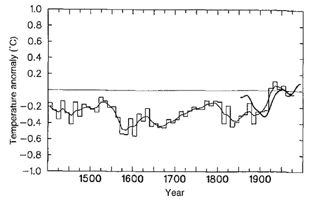
Figure 3.20: Decadal summer temperature index for the Northern Hemisphere, from Bradley and Jones (1993), up to 1970–1979. The record is based on the average of 16 proxy summer temperature records from North America, Europe and east Asia. The smooth one was created using an approximately 50-year Gaussian filter. Recent instrumental data for Northern Hemisphere summer temperature anomalies (over land and ocean) are also plotted (thick line). The instrumental record is probably biased high in the mid-19th century, because of exposures differing from current techniques (for example, Parker, 1994b).
NOTE: The following two curves show the proxy temperature reconstruction from the first and second IPCC reports for the overlapping timeframe (1400–2000):
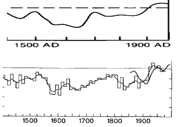
[119] Report: “Climate Change 2001: The Scientific Basis.” Edited by J.T. Houghton and others. World Meteorological Organization/United Nations Environment Programme, Intergovernmental Panel on Climate Change, 2001. <www.ipcc.ch>
Chapter 2: “Observed Climate Variability and Change.” By C.K. Folland and others. Pages 99–182.
The graph is displayed in Section 2.3.2.1 (“Palaeoclimate proxy indicators”) with this caption: “Figure 2.20: Millennial Northern Hemisphere (NH) temperature reconstruction (blue) and instrumental data (red) from AD 1000 to 1999, adapted from Mann and others (1999). Smoother version of NH series (black), linear trend from AD 1000 to 1850 (purple-dashed) and two standard error limits (grey shaded) are shown.”
Section 2.3.1 (Background):
Since the SAR [IPCC Second Assessment Report], a number of studies based on considerably expanded databases of palaeoclimate information have allowed more decisive conclusions about the spatial and temporal patterns of climate change in past centuries. A number of important advances have been in key areas such as ice core palaeoclimatology (for example, White and others, 1998a), dendroclimatology (for example, Cook, 1995; Briffa and others, 1998b), and geothermal palaeo-temperature estimation (for example, Pollack and others, 1998). Moreover, the latest studies based on global networks of “multi-proxy” data have proved particularly useful for describing global or hemispheric patterns of climate variability in past centuries (for example, Bradley and Jones, 1993; Hughes and Diaz, 1994; Mann and others, 1995; Fisher, 1997; Overpeck and others, 1997; Mann and others, 1998, 1999).
Section 2.3.3 (Was there a “Little Ice Age” and a “Medieval Warm Period”?):
[T]he conventional terms of “Little Ice Age” and “Medieval Warm Period” appear to have limited utility in describing trends in hemispheric or global mean temperature changes in past centuries. With the more widespread proxy data and multi-proxy reconstructions of temperature change now available, the spatial and temporal character of these putative climate epochs can be reassessed.
[120]
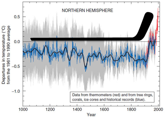
[121] Report: “Climate Change 2001: The Scientific Basis.” Edited by J.T. Houghton and others. World Meteorological Organization/United Nations Environment Programme, Intergovernmental Panel on Climate Change, 2001. <www.ipcc.ch>
Chapter 2: “Observed Climate Variability and Change.” By C.K. Folland and others. Pages 99–182.
Page 134: “Figure 2.20: Millennial Northern Hemisphere (NH) temperature reconstruction (blue) and instrumental data (red) from AD 1000 to 1999, adapted from Mann and others (1999). Smoother version of NH series (black), linear trend from AD 1000 to 1850 (purple-dashed) and two standard error limits (grey shaded) are shown.”
[122] Synthesis report: “Climate Change 2001: Summary for Policy Makers.” Edited by Robert T. Watson and others. World Meteorological Organization/United Nations Environment Programme, Intergovernmental Panel on Climate Change, 2001. <www.ipcc.ch>
Page 34:
Figure SPM-10b: Variations of the Earth’s surface temperature: years 1000 to 2100. From year 1000 to year 1860 variations in average surface temperature of the Northern Hemisphere are shown (corresponding data from the Southern Hemisphere not available) reconstructed from proxy data (tree rings, corals, ice cores, and historical records). The line shows the 50-year average, the grey region the 95% confidence limit in the annual data.
[123] Paper: “Northern Hemisphere Temperatures During the Past Millennium: Inferences, Uncertainties, and Limitations.” By Michael E. Mann, Raymond S. Bradley, and Malcolm K. Hughes. Geophysical Research Letters, March 15, 1999. <www.meteo.psu.edu>
Pages 1–2:
Recently, Mann and others [1998—henceforth “MBH98”] reconstructed yearly global surface temperature patterns back in time through the calibration of multiproxy networks against the modern temperature record. … We here apply the methodology detailed by MBH98 to the sparser proxy data network available prior to AD 1400, to critically revisit this issue, extending NH [Northern Hemisphere] reconstructions as far back as is currently feasible.
[124] Paper: “Global-Scale Temperature Patterns and Climate Forcing Over the Past Six Centuries.” By Michael E. Mann, Raymond S. Bradley, and Malcolm K. Hughes. Nature, April 23, 1998. Pages 779–787. <www.geo.umass.edu>
[125] Report: “Climate Change 2001: The Scientific Basis.” Edited by J.T. Houghton and others. World Meteorological Organization/United Nations Environment Programme, Intergovernmental Panel on Climate Change, 2001. <www.ipcc.ch>
Chapter 2: “Observed Climate Variability and Change.” By C.K. Folland and others. Pages 99–182.
Page 134.
[126] Synthesis report: “Climate Change 2001: Summary for Policy Makers.” Edited by Robert T. Watson and others. World Meteorological Organization/United Nations Environment Programme, Intergovernmental Panel on Climate Change, 2001. <www.ipcc.ch>
Page 34.
[127] Report: “Climate Change 2001: The Scientific Basis.” Edited by J.T. Houghton and others. World Meteorological Organization/United Nations Environment Programme, Intergovernmental Panel on Climate Change, 2001. “Summary for Policymakers.” Based on a draft prepared by Daniel L. Albritton and others. <www.ipcc.ch>
Pages 3 and 29.
[128] Paper: “Corrections to the Mann et. al. (1998) Proxy Data Base and Northern Hemispheric Average Temperature Series.” By Stephen McIntyre and Ross McKitrick. Energy & Environment, November 6, 2003. Pages 751–771. <climateaudit.files.wordpress.com>
Page 751:
The data set of proxies of past climate used in Mann, Bradley and Hughes (1998, “MBH98” hereafter) … contains collation errors, unjustifiable truncation or extrapolation of source data, obsolete data, geographical location errors, incorrect calculation of principal components and other quality control defects. … The particular “hockey stick” shape derived in the MBH98 proxy construction … is primarily an artefact of poor data handling, obsolete data and incorrect calculation of principal components.
[129] Paper: “Robustness of the Mann, Bradley, Hughes Reconstruction of Northern Hemisphere Surface Temperatures: Examination of Criticisms Based on the Nature and Processing of Proxy Climate Evidence.” By Eugene R. Wahl and Caspar M. Ammann. Climatic Change, November 2007. Pages 33–69. <link.springer.com>
Page 33: “Altogether new reconstructions over 1400–1980 are developed in both the indirect and direct analyses, which demonstrate that the Mann and others reconstruction is robust against the proxy-based criticisms addressed.”
[130] “Response of Dr. Edward Wegman to Questions Posed by the Honorable Mr. Bart Stupak in Connection with Testimony to the Subcommittee on Oversight and Investigations.” October 1, 2006. <www.justfacts.com>
“The MBH98 [Mann, Bradley and Hughes, 1998] methodology puts undue emphasis on those proxies that do exhibit the hockey-stick shape and this is the fundamental flaw. Indeed, it is not clear that the hockey-stick shape is even a temperature signal because all the confounding variables have not been removed.”
[131] Letter to Joe Barton (Chairman of the U.S. House Committee on Energy and Commerce) and Ed Whitfield (Chairman of the Subcommittee on Oversight and Investigations). By Michael E. Mann. July 15, 2005. <www.realclimate.org>
“This letter responds to your letter of June 23, 2005, which seeks information on issues relating to my research on the historical record of temperatures and climate change. Your letter lays out a number of ‘concerns’ about the research my colleagues and I have conducted about global warming.”
[132] See the section of this research on ClimateGate.
[133] Webpage: “American Tradition Institute v. University of Virginia (Dr. Michael Mann).” American Tradition Institute, May 16, 2011.
On May 16, 2011, American Tradition Institute’s Environmental Law Center and Virginia Delegate Robert Marshall asked a Prince William County judge, under the Commonwealth’s Freedom of Information Act, to expedite the release of documents withheld by the University of Virginia that pertain to the work of its former environmental sciences assistant professor Dr. Michael Mann. …
The emails and other documents ATI [American Tradition Institute] seeks relate to claims made by Dr. Mann to obtain, and claim payment under, certain taxpayer-funded grants. Mann, currently at Pennsylvania State University, worked at the UVA’s [University of Virginia’s] Department of Environmental Sciences when he produced what was hailed at the time as the “smoking gun” affirming the theory of catastrophic man-made global warming, and the policy agenda demanded by its proponents. After a persistent cloud of controversy—much of which was affirmed by the “ClimateGate” leak of 2009—this notorious “Hockey Stick” graph disappeared from the UN’s Intergovernmental Panel on Climate Change (IPCC) Assessment Reports, the perch that launched it.
[134] Article: “Ruling Alters Climate-Papers Fight.” By Paige Winfield Cunningham. Washington Times, May 25, 2011. <www.washingtontimes.com>
“Mr. Marshall, Prince William Republican, requested the documents through the Freedom of Information Act, while Mr. Cuccinelli subpoenaed them. Mr. Cuccinelli said an order issued Tuesday in Prince William County Circuit Court that grants Mr. Marshall’s request could affect his own appeal to the state Supreme Court to reverse a previous ruling in favor of the university.”
[135] Paper: “A Statistical Analysis of Multiple Temperature Proxies: Are Reconstructions of Surface Temperatures Over the Last 1000 Years Reliable?” By Blakeley B. McShane and Abraham J. Wyner. Annals of Applied Statistics, April 20, 2011. <arxiv.org>
Pages 3–4:
Fig. 1. … based on the work by Mann, Bradley and Hughes (1999). This figure has sometimes been referred to as the “hockey stick.” Source: IPCC (2001). …
It is not necessary to know very much about the underlying methods to see that graphs such as Figure 1 are problematic as descriptive devices. … the blue curve closely matches the red curve during the period 1902 AD to 1980 AD because this period has served as the training data and therefore the blue curve is calibrated to the red during it (note also the red curve is plotted from 1902 AD to 1998 AD). This sets up the erroneous visual expectation that the reconstructions are more accurate than they really are.
Page 7: “[F]or the remainder of the paper, we work entirely with the data from Mann and others (2008).”
Pages 36–37:
Still, it seems there is simply not enough signal in the proxies to detect either the high levels of or the sharp run-up in temperature seen in the 1990s. This is disturbing: if a model cannot predict the occurrence of a sharp run-up in an out-of-sample block which is contiguous with the in-sample training set, then it seems highly unlikely that it has power to detect such levels or run-ups in the more distant past.
Page 39: “Our backcasting methods, which track quite closely the methods applied most recently in Mann (2008) to the same data, are unable to catch the sharp run up in temperatures recorded in the 1990s, even in-sample.”
Page 40: “It is not clear that the proxies currently used to predict temperature are even predictive of it at the scale of several decades let alone over many centuries.”
[136] Paper: “Hockey Sticks, Principal Components, and Spurious Significance.” By Stephen Mcintyre and Ross Mckitrick. Geophysical Research Letters, February 12, 2005. <citeseerx.ist.psu.edu>
Pages 1–2:
The “hockey stick” shaped temperature reconstruction of Mann and others (1998, 1999) has been widely applied. However it has not been previously noted in print that, prior to their principal components (PCs) analysis on tree ring networks, they carried out an unusual data transformation which strongly affects the resulting PCs. Their method, when tested on persistent red noise, nearly always produces a hockey stick shaped first principal component (PC1) and overstates the first eigenvalue. …
[The computer] code … contains an unusual data transformation prior to PC calculation that has never been reported in print. … Since PC algorithms choose weights that maximize variance, the method reallocates variance so that hockey stick shaped series get overweighted. …
In effect, the MBH98 [Mann, Bradley, Hughes, 1998] data transformation results in the PC algorithm mining the data for hockey stick patterns. In a network of persistent red noise, there will be some series that randomly “trend” up or down during the ending sub-segment of the series (as well as other subsegments). … these spurious “trends” in a closing segment are sufficient for the MBH98 method, when applied to a network of red noise, to yield hockey stick PC1s, even though the underlying data generating process has no trend component.
Page 3: “The most heavily weighted site in the MBH98 PC1, Sheep Mountain, is a bristlecone pine site with the most pronounced hockey stick shape (1.6 s) in the network; it receives over 390 times the weight of the least weighted site, Mayberry Slough, whose hockey stick index is near 0.”
[137] “Response of Dr. Edward Wegman to Questions Posed by the Honorable Mr. Bart Stupak in Connection with Testimony to the Subcommittee on Oversight and Investigations.” October 1, 2006. <www.justfacts.com>
In order to set the context for my responses, I would like to make a few observations. I have been a professional statistician for some 38 years. I have served as editor of the Journal of the American Statistical Association and served as coordinating editor, associate editor, member of the editorial board and a number of other editorial roles for many journals during this time period. I am currently on the Board of Directors of the American Statistical Association as the publications representative and will become the Chair of their Publications Committee as of 1 January, 2007. …
To reiterate our testimony, the decentering process as used in MBH98 [Mann, Bradley Hughes, 1998] and MBH99 selectively prefers to emphasize the hockey stick shape. This is because the decentering increases the apparent variance of hockey sticks and principal component methods attempt to find components with the largest explainable variance. If the variance is artificially increased by decentering, then the principal component methods will “data mine” for those shapes. In other words, the hockey stick shape must be in the data to start with or the CFR [climate field reconstruction] methodology would not pick it up. What we have shown both analytically and graphically in Figure 4.6 is that using the CFR methodology, just one signal when decentered will overwhelm 69 independent noise series. The point is that if all 70 proxies contained the same temperature signal, then it wouldn’t matter which method one used. But this is very far from the case. Most proxies do not contain the hockey-stick signal. The MBH98 methodology puts undue emphasis on those proxies that do exhibit the hockey-stick shape and this is the fundamental flaw. Indeed, it is not clear that the hockey-stick shape is even a temperature signal because all the confounding variables have not been removed.
[138] See the two footnotes above for vital context in understanding the next three footnotes.
[139] Book: Making Sense of Data II: A Practical Guide to Data Visualization, Advanced Data Mining Methods, and Applications. By Glenn J. Myatt and Wayne P. Johnson. Wiley, 2009.
Page 127:
Principal component analysis produces the same number of components as variables. However, each principal component accounts for a different amount of variation in the data set. In fact, only a small number of principal components usually account for the majority of variation in the data. The first principal component accounts for the most variation in the data. The second principal component accounts for the second highest amount of variation in the data, and so on.
[140] Book: Principal Components Analysis. By George H. Dunteman. SAGE Publications, 1989.
Page 10:
Principal components analysis searches for a few uncorrelated linear combinations of the original variables that capture most of the information in the original variables. … The linear composites (principal components) are ordered with respect to their variation so that the first few account for most of the variation present in the original variables, or equivalently, the first few principal components together have, overall, the highest possible squared multiple correlations with each of the original variables.
Geometrically, the first principal component is the line of closest fit the n observations in the p dimensional variable space.
[141] “Response of Dr. Edward Wegman to Questions Posed by the Honorable Mr. Bart Stupak in Connection with Testimony to the Subcommittee on Oversight and Investigations.” October 1, 2006. <www.justfacts.com>
Pages 10–14:
The Wahl and Ammann paper [defending the hockey stick graph and cited in the note below†] came to our attention relatively late in our deliberations, but was considered by us. Some immediate thoughts we had on Wahl and Ammann was that Dr. Mann lists himself as a Ph.D. coadvisor to Dr. Ammann on his resume. As I testified in the second hearing, the work of Dr. Ammann can hardly be thought to be an unbiased independent report. It would have been more convincing had this paper been written by a totally independent authority, but alas this is not the case. The Wahl and Ammann paper is largely an attempt to refute the criticisms of McIntyre and McKitrick (MM). …
It is our understanding that when using the same proxies as and the same methodology as MM, Wahl and Ammann essentially reproduce the MM curves. Thus, far from disproving the MM work, they reinforce the MM work. The debate then is over the proxies and the exact algorithms as it always has been. …
[Question 10b:] Do you agree or disagree with Wahl and Ammann’s finding that the time period used to center the data does not significantly affect the results reported in the MBH98 [Mann, Bradley and Hughes] paper? If you disagree, please state the basis for your disagreement.
Answer: We do disagree. The fundamental issue focuses on the North American Tree Ring proxy series, which Wahl and Ammann admit are problematic in carrying temperature data. In the original MBH [Mann, Bradley, Hughes; i.e., hockey stick] decentered series, the hockey-stick shape emerged in the PC1 [first principal component] series because of reasons we have articulated in both our report and our testimony. In the original MBH papers, it was argued that this PC1 proxy was sufficient. …
Without attempting to describe the technical detail, the bottom line is that, in the MBH original, the hockey stick emerged in PC1 from the bristlecone/foxtail pines. If one centers the data properly the hockey stick does not emerge until PC4. Thus, a substantial change in strategy is required in the MBH reconstruction in order to achieve the hockey stick, a strategy which was specifically eschewed in MBH [see note below †]. In Wahl and Ammann’s own words, the centering does significantly affect the results.
[Question 10c:] Dr. Gulledge included in his testimony a slide showing the graph of W A [Wahl and Ammann] emulation of the MBH and MBH-corrected for decentering and the Gaspe tree-ring series. Were you aware of their reanalysis of MBH99 prior to the time you finalized your report? Do you agree or disagree with their reanalysis of MBH99? If you disagree, please state the basis for your disagreement.
Answer: Yes, we were aware of the Wahl and Ammann simulation. We continue to disagree with the reanalysis for several reasons. Even granting the unbiasedness of the Wahl and Ammann study in favor of his advisor’s methodology and the fact that it is not a published refereed paper, the reconstructions mentioned by Dr. Gulledge, and illustrated in his testimony, fail to account for the effects of the bristlecone/foxtail pines. Wahl and Ammann reject this criticism of MM based on the fact that if one adds enough principal components back into the proxy, one obtains the hockey stick shape again. This is precisely the point of contention. It is a point we made in our testimony and that Wahl and Ammann make as well. A cardinal rule of statistical inference is that the method of analysis must be decided before looking at the data. The rules and strategy of analysis cannot be changed in order to obtain the desired result. Such a strategy carries no statistical integrity and cannot be used as a basis for drawing sound inferential conclusions.
NOTES:
[142] Paper: “A Statistical Analysis of Multiple Temperature Proxies: Are Reconstructions of Surface Temperatures Over the Last 1000 Years Reliable?” By Blakeley B. McShane and Abraham J. Wyner. Annals of Applied Statistics, April 20, 2011. <arxiv.org>
Pages 4–5: “A careful viewer would know to temper such expectations by paying close attention to the reconstruction error bars given by the wide gray regions. However, even these are misleading because these are, in fact, pointwise confidence intervals and not confidence curves for the entire sample path of surface temperature. Furthermore, the gray regions themselves fail to account for model uncertainty.”
[143] Report: “Surface Temperature Reconstructions for the Last 2,000 Years.” By Gerald R. North and others. National Academy of Sciences, National Research Council, Committee on Surface Temperature Reconstructions for the Last 2,000 Years. National Academies Press, 2006. <www.nap.edu>
Page 15:
FIGURE O-4 Multiproxy reconstruction of Northern Hemisphere surface temperature variations over the past millennium (blue), along with 50-year average (black), a measure of the statistical uncertainty associated with the reconstruction (grey), and instrumental surface temperature data for the last 150 years (red), based on the work by Mann and others (1999). This figure has sometimes been referred to as the “hockey stick.” SOURCE: IPCC (2001).
Page 16:
Despite the wide error bars, Figure O-4 was misinterpreted by some as indicating the existence of one ‘definitive’ reconstruction with small century-to-century variability prior to the mid-19th century. It should also be emphasized that the error bars in this particular figure, and others like it, do not reflect all of the uncertainties inherent in large-scale surface temperature reconstructions based on proxy data.
[144] See the section of this research on the “hide the decline“ emails.
[145] Report: “Climate Change 2007: The Physical Science Basis.” Edited by S. D. Solomon and others. World Meteorological Organization/United Nations Environment Programme, Intergovernmental Panel on Climate Change. Cambridge University Press, 2007. <www.ipcc.ch>
Chapter 6: “Palaeoclimate.” By Eystein Jansen and others. Pages 433–497. <www.ipcc.ch>
Page 467: “Figure 6.10. Records of NH [Northern Hemisphere] temperature variation during the last 1.3 kyr [1,300 years]. … (b) Reconstructions using multiple climate proxy records, identified in Table 6.1, including three records … shown in the TAR [Third Assessment Report], and the HadCRUT2v instrumental temperature record in black.”
Page 469: “There are far from sufficient data to make any meaningful estimates of global medieval warmth (Figure 6.11). There are very few long records with high temporal resolution data from the oceans, the tropics or the SH [Southern Hemisphere].”
[146] Report: “Climate Change 2007: The Physical Science Basis.” Edited by S. D. Solomon and others. World Meteorological Organization/United Nations Environment Programme, Intergovernmental Panel on Climate Change. Cambridge University Press, 2007.
Chapter 6: “Palaeoclimate.” By Eystein Jansen and others. Pages 433–497. <www.ipcc.ch>
Page 468:
Box 6.4, Figure 1. The heterogeneous nature of climate during the “Medieval Warm Period” is illustrated by the wide spread of values exhibited by the individual records that have been used to reconstruct NH mean temperature. These consist of individual, or small regional averages of, proxy records collated from those used by Mann and Jones (2003), Esper and others (2002) and Luckman and Wilson (2005), but exclude shorter series or those with no evidence of sensitivity to local temperature. These records have not been calibrated here, but each has been smoothed with a 20-year filter and scaled to have zero mean and unit standard deviation over the period 1001 to 1980.
[147] Report: “Climate Change 2013: The Physical Science Basis.” Edited by Thomas Stocker and others. Intergovernmental Panel on Climate Change, 2013. <www.climatechange2013.org>
Chapter 5: “Information From Paleoclimate Archives.” By Valerie Masson-Delmotte and others. Pages 383–464. <www.ipcc.ch>
Page 409:
Figure 5.7 Reconstructed (a) Northern Hemisphere and (b) Southern Hemisphere, and (c) global annual temperatures during the last 2000 years. Individual reconstructions (see Appendix 5.A.1 for further information about each one) are shown as indicated in the legends, grouped by colour according to their spatial representation (red: land-only all latitudes; orange: land-only extratropical latitudes; light blue: land and sea extra-tropical latitudes; dark blue: land and sea all latitudes) and instrumental temperatures shown in black (Hadley Centre/ Climatic Research Unit (CRU) gridded surface temperature-4 data set (HadCRUT4) land and sea, and CRU Gridded Dataset of Global Historical Near-Surface Air TEMperature Anomalies Over Land version 4 (CRUTEM4) land-only; Morice and others, 2012). All series represent anomalies (°C) from the 1881–1980 mean (horizontal dashed line) and have been smoothed with a filter that reduces variations on time scales less than about 50 years.
Page 411:
Reconstructing NH [Northern Hemisphere], SH [Southern Hemisphere] or global-mean temperature variations over the last 2000 years remains a challenge due to limitations of spatial sampling, uncertainties in individual proxy records and challenges associated with the statistical methods used to calibrate and integrate multi-proxy information (Hughes and Ammann, 2009; Jones and others, 2009; Frank and others, 2010a). …
The fundamental limitations for deriving past temperature variability at global/hemispheric scales are the relatively short instrumental period and the number, temporal and geographical distribution, reliability and climate signal of proxy records (Jones and others, 2009). The database of high-resolution proxies has been expanded since AR4 [i.e., the Fourth IPCC Assessment Report] (Mann and others, 2008; Wahl and others, 2010; Neukom and Gergis, 2011; Pages 2k Consortium, 2013), but data are still sparse in the tropics, SH and over the oceans (see new developments in Section 5.5). Integration of low-resolution records (for example, marine or some lake sediment cores and some speleothem records) with high-resolution tree-ring, ice core and coral records in global/hemispheric reconstructions is still challenging. Dating uncertainty, limited replication and the possibility of temporal lags in low-resolution records (Jones and others, 2009) make regression-based calibration particularly difficult (Christiansen and others, 2009) and can be potentially best addressed in the future with Bayesian hierarchical models (Tingley and others, 2012). The short instrumental period and the paucity of proxy data in specific regions may preclude obtaining accurate estimates of the covariance of temperature and proxy records (Juckes and others, 2007), impacting the selection and weighting of proxy records in global/hemispheric reconstructions (Bürger, 2007; Osborn and Briffa, 2007; Emile-Geay and others, 2013b) and resulting in regional errors in climate field reconstructions (Smerdon and others, 2011).
Page 412:
Limitations in proxy data and reconstruction methods suggest that published uncertainties [in the academic literature] will underestimate the full range of uncertainties of large-scale temperature reconstructions (see Section 5.3.5.1). While this has fostered debate about the extent to which proxy-based reconstructions provide useful climate information (for example, McShane and Wyner, 2011 and associated comments and rejoinder), it is well established that temperature and external forcing signals are detectable in proxy reconstructions (Sections 5.3.5.3 and 10.7.2).
[148] Report: “Climate Change 2021: The Physical Science Basis.” Edited by V. Masson-Delmotte and others. Intergovernmental Panel on Climate Change. Cambridge University Press, 2021. <report.ipcc.ch>
“Summary for Policymakers.” By Valérie Masson-Delmotte and others. Pages 3–31. <www.ipcc.ch>
Page 6:
Human influence has warmed the climate at a rate that is unprecedented in at least the last 2000 years
Changes in global surface temperature relative to 1850–1900
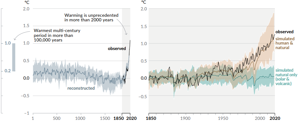
Panel (a) Changes in global surface temperature reconstructed from paleoclimate archives (solid grey line, years 1–2000) and from direct observations (solid black line, 1850–2020), both relative to 1850–1900 and decadally averaged. … The grey shading with white diagonal lines shows the very likely ranges for the temperature reconstructions.
[149] Report: “Climate Change 2021: The Physical Science Basis.” Edited by V. Masson-Delmotte and others. Intergovernmental Panel on Climate Change. Cambridge University Press, 2021. <report.ipcc.ch>
“Technical Summary.” By Paola A. Arias and others. Pages 35–144. <www.ipcc.ch>
Pages 61–62:
(a) Global surface temperatures are more likely than not unprecedented in the past 125,000 years
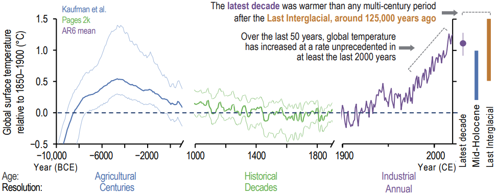
Figure 1 | Earth’s surface temperature history and future with key findings annotated within each panel. … The intent of this figure is to show global surface temperature observed changes from the Holocene to now, and projected changes. (a) Global surface temperature over the Holocene divided into three time scales: (i) 12,000 to 1000 years ago (10,000 BCE to 1000 CE) in 100-year time steps, (ii) 1000 to 1900 CE, 10-year smooth, and (iii) 1900 to 2020 CE (mean of four datasets in panel c). Bold lines show the median of the multi-method reconstruction, with 5% and 95% percentiles of the ensemble members (thin lines). Vertical bars are 5–95th percentile ranges of estimated global surface temperature for the Last Interglacial and mid-Holocene (medium confidence) (Section 2.3.1.1). All temperatures are relative to 1850–1900.
[150] Report: “Climate Change 2021: The Physical Science Basis.” Edited by V. Masson-Delmotte and others. Intergovernmental Panel on Climate Change. Cambridge University Press, 2021. <report.ipcc.ch>
[151] Report: “Climate Change 2021: The Physical Science Basis.” Edited by V. Masson-Delmotte and others. Intergovernmental Panel on Climate Change. Cambridge University Press, 2021. <report.ipcc.ch>
Chapter 2: “Changing State of the Climate System.” by Sergey K. Gulev and others. Pages 287–422. <www.ipcc.ch>
Page 315:
For the LIG [Last Interglacial] … a major new compilation of marine proxy data (Turney and others, 2020) from 203 sites indicates that the average SST [sea surface temperatures] from 129–125 ka [thousand years ago] was 1.0°C ± 0.2°C (2 SD [standard deviation]) warmer than 1850–1900 (reported relative to 1981–2010 and adjusted here by 0.8°C). … In summary, GMST [global mean surface temperature] during the warmest millennia of the LIG (within the interval of around 129–125 ka) is estimated to have reached 0.5°C–1.5°C higher values than the 1850–1990 reference period (medium confidence).
New GMST reconstructions for the LGM [Last Glacial Maximum] fall near the middle of AR5’s very likely range, which was based on a combination of proxy reconstructions and model simulations. Two of these new reconstructions use marine proxies to reconstruct global SST that were scaled to GMST based on different assumptions. One indicates that GMST was 6.2 [4.5 to 8.1°C; 95% range] cooler than the late Holocene average (Snyder, 2016), and the other, 5.7°C ± 0.8°C (2 SD) cooler than the average of the first part of the Holocene (10–5 ka) (Friedrich and Timmermann, 2020). A third new estimate (Tierney and others, 2020) uses a much larger compilation of marine proxies along with a data-assimilation procedure, rather than scaling, to reconstruct a GMST of 6.1°C ± 0.4°C (2 SD) cooler than the late Holocene. Assuming that the 1850–1900 reference period was 0.2°C and 0.4°C cooler than the late and first part of the Holocene, respectively (Kaufman and others, 2020a), the midpoints of these three new GMST reconstructions average –5.8°C relative to 1850–1900. … A major new pollen-based data-assimilation reconstruction averages 6.9°C cooler over northern extratropical land (Cleator and others, 2020). …
In summary, GMST is estimated to have been 5°C–7°C lower during the LGM (around 23–19 ka [thousand years ago]) compared with 1850–1900 (medium confidence).
For the LDT [Last Deglacial Termination] … no new large-scale studies have been published since AR5 (Shakun and others, 2012) to further assess the rate of GMST change during this period of rapid global warming (estimated at 1°C–1.5°C per kyr). The reconstruction of Shakun and others (2012) was based primarily on SST records and therefore underrepresents the change in GMST during the LDT. Temperature over Greenland increased by about ten times that rate during the centuries of most rapid warming (Jansen and others, 2020).
2.3.1.1.2 Temperatures of the post-glacial period (past 7000 years) …
A multi-method reconstruction (Kaufman and others, 2020a) based on a quality-controlled, multi-proxy synthesis of paleo-temperature records from 470 terrestrial and 209 marine sites globally (Kaufman and others, 2020b) indicates that the median GMST of the warmest two-century-long interval was 0.7 [0.3 to 1.8] °C warmer than 1800–1900 (which averaged 0.03°C colder than 1850–1900; PAGES 2k Consortium, 2019), and was centred around 6.5 ka. This is similar to Marcott and others (2013), which is based on a smaller dataset (73 sites) and different procedures to estimate a maximum warmth of 0.8°C ± 0.3°C (2 SD) at around 7.0 ka, adjusted here by adding 0.3°C to account for differences in reference periods.
Page 317:
In addition, a major new global compilation of multiproxy, annually resolved paleo-temperature records for the CE (PAGES 2k Consortium, 2017) has been analysed using a variety of statistical methods for reconstructing temperature (PAGES 2k Consortium, 2019). The median of the multi-method GMST reconstruction from this synthesis … generally agrees with the AR5 assessment, while affording more robust estimates of the following major features of GMST during the CE: (i) an overall millennial-scale cooling trend of –0.18 [–0.28 to 0.00] °C kyr–1 prior to 1850; (ii) a multi-centennial period of relatively low temperature beginning around the 15th century, with GMST averaging –0.03 [–0.30 to 0.06] °C between 1450 and 1850 relative to 1850–1900; (iii) the warmest multi-decadal period occurring most recently; and (iv) the rate of warming during the second half of the 20th century (from instrumental data) exceeding the 99th percentile of all 51-year trends over the past 2 kyr. Moreover, the new proxy data compilation shows that the warming of the 20th century was more spatially uniform than any other century-scale temperature change of the CE (medium confidence) (Neukom and others, 2019). A new independent temperature reconstruction extending back to 1580 is based on an expanded database of subsurface borehole temperature profiles, along with refined methods for inverse modelling (Cuesta-Valero and others, 2021).
Pages 376–377:
Development of new techniques and exploitation of existing and new proxy sources may help address challenges around the low temporal resolution of most paleoclimate proxy records, particularly prior to the Common Era, and ambiguities around converting paleoclimate proxy data into estimates of climate-relevant variables. Conversions rely upon important proxy-specific assumptions and biases can be large due to limited accounting of seasonality, non-climatic effects, or the influence of multiple climate variables. These challenges currently limit the ability to ascertain the historical unusualness of recent directly observed climate changes for many indicators. …
Contradictory lines of evidence exist between observations and models on the relationship between the rates of warming in GMST and GSAT, compounded by limitations in theoretical understanding. Improvements in air temperature datasets over the ocean and an improved understanding of the representation of the lowermost atmosphere over the ocean in models would reduce uncertainty in assessed changes in GSAT.
[152] Paper: “Seeing the Wood From the Trees.” By Keith R. Briffa and Timothy J. Osborn. Science, May 7, 1999. Pages 926–927. <www.meteo.psu.edu>
An uninformed reader would be forgiven for interpreting the similarity between the 1000-year temperature curve of Mann and others and a variety of others also representing either temperature change over the NH [Northern Hemisphere] as a whole or a large part of it (see the figure) as strong corroboration of their general validity, and, to some extent, this may well be so. Unfortunately, very few of the series are truly independent: There is a degree of common input to virtually every one, because there are still only a small number of long, well-dated, high-resolution proxy records.
[153] Report: “Climate Change 2007: The Physical Science Basis.” Edited by S. D. Solomon and others. World Meteorological Organization/United Nations Environment Programme, Intergovernmental Panel on Climate Change. Cambridge University Press, 2007.
Chapter 6: “Palaeoclimate.” By Eystein Jansen and others. Pages 433–497. <www.ipcc.ch>
Page 471: “[T]hese new records are not entirely independent reconstructions inasmuch as there are some predictors (most often tree ring data and particularly in the early centuries) that are common between them, but in general, they represent some expansion in the length and geographical coverage of the previously available data (Figures 6.10 and 6.11).”
[154] Paper: “Extra-Tropical Northern Hemisphere Land Temperature Variability Over the Past 1000 Years.” By Edward R. Cook and others. Quaternary Science Reviews, November 2004. Pages 2063–2074. <www.sciencedirect.com>
Page 2071: “The re-calibrated mean RCS [Regional Curve Standardization method] tree-ring record probably represents the best reconstruction of past land-only, extra-tropical NH [Northern Hemisphere] annual temperatures that is practical to extract from it at this time.”
Page 2065: “Fig. 2. Map of the Esper et. al. (2002) tree-ring sites. Each solid red dot represents one of the 14 sites used. The six circled-sites are those that extend back to AD 831, the beginning of the ECS [Esper, Cook, and Schweingruber, 2002] record.”
NOTES:
[155] Paper: “A Statistical Analysis of Multiple Temperature Proxies: Are Reconstructions of Surface Temperatures Over the Last 1000 Years Reliable?” By Blakeley B. McShane and Abraham J. Wyner. Annals of Applied Statistics, April 20, 2011. <arxiv.org>
Page 1:
In this paper, we assess the reliability of such reconstructions and their statistical significance against various null models. We find that the proxies do not predict temperature significantly better than random series generated independently of temperature. Furthermore, various model specifications that perform similarly at predicting temperature produce extremely different historical backcasts. Finally, the proxies seem unable to forecast the high levels of and sharp run-up in temperature in the 1990s either in-sample or from contiguous holdout blocks, thus casting doubt on their ability to predict such phenomena if in fact they occurred several hundred years ago.
Pages 6–7: “[H]enceforth and for the remainder of the paper, we work entirely with the data from Mann and others (2008). … This is by far the most comprehensive publicly available database of temperatures and proxies collected to date.”
Page 18: “In other words, our model performs better when using highly autocorrelated noise rather than proxies to ‘predict’ temperature. The real proxies are less predictive than our ‘fake’ data.”
[156] Report: “Climate Change 1995: The Science of Climate Change.” Edited by J.T. Houghton and others. World Meteorological Organization/United Nations Environment Programme, Intergovernmental Panel on Climate Change. Cambridge University Press, 1996. <www.ipcc.ch>
Chapter 8: “Detection of Climate Change and Attribution of Causes.” By B.D. Santer and others. Pages 407–444.
Page 419: “In order to produce a reconstruction, the raw data are generally subjected to some form of statistical manipulation, through which only part of the original climate information can be retrieved (typically less than 50%).”
[157] Report: “Climate Change 1995: The Science of Climate Change.” Edited by J.T. Houghton and others. World Meteorological Organization/United Nations Environment Programme, Intergovernmental Panel on Climate Change. Cambridge University Press, 1996. <www.ipcc.ch>
Chapter 8: “Detection of Climate Change and Attribution of Causes.” By B.D. Santer and others. Pages 407–444.
Page 419: “Most temperature reconstructions, for example, are seasonally specific, rather than providing some integrated response to annual-mean conditions.”
[158] Paper: “Extra-Tropical Northern Hemisphere Land Temperature Variability Over the Past 1000 Years.” By Edward R. Cook and others. Quaternary Science Reviews, November 2004. Pages 2063–2074. <www.sciencedirect.com>
Page 2073: “We have argued that this reconstruction is best interpreted as an expression of land-only, extra-tropical NH (Northern Hemisphere) temperature variability. It probably best reflects warm-season-weighted temperatures, but an annual temperature model can also be used as a reasonable approximation.”
[159] Report: “Surface Temperature Reconstructions for the Last 2,000 Years.” By Gerald R. North and others. National Academy of Sciences, National Research Council, Committee on Surface Temperature Reconstructions for the Last 2,000 Years. National Academies Press, 2006. <www.nap.edu>
Page 15:
FIGURE O-4 Multiproxy reconstruction of Northern Hemisphere surface temperature variations over the past millennium (blue), along with 50-year average (black), a measure of the statistical uncertainty associated with the reconstruction (grey), and instrumental surface temperature data for the last 150 years (red), based on the work by Mann and others (1999). This figure has sometimes been referred to as the “hockey stick.” Source: IPCC (2001).
Page 16:
Despite the wide error bars, Figure O-4 was misinterpreted by some as indicating the existence of one “definitive” reconstruction with small century-to-century variability prior to the mid-19th century. It should also be emphasized that the error bars in this particular figure, and others like it, do not reflect all of the uncertainties inherent in large-scale surface temperature reconstructions based on proxy data.
[160] “Ad Hoc Committee Report on the ‘Hockey Stick’ Global Climate Reconstruction.” By Edward J. Wegman and others. Prepared for the U.S. House of Representatives, Chairman of the Committee on Energy and Commerce and Chairman of the Subcommittee on Oversight and Investigations, July 12, 2006. <bit.ly>
Page 2:
This committee, composed of Edward J. Wegman (George Mason University), David W. Scott (Rice University), and Yasmin H. Said (The Johns Hopkins University), has reviewed the work of both articles, as well as a network of journal articles that are related either by authors or subject matter, and has come to several conclusions and recommendations. This Ad Hoc Committee has worked pro bono, has received no compensation, and has no financial interest in the outcome of the report.
Page 6: “Especially when massive amounts of public monies and human lives are at stake, academic work should have a more intense level of scrutiny and review. It is especially the case that authors of policy-related documents like the IPCC report, Climate Change 2001: The Scientific Basis, should not be the same people as those that constructed the academic papers.”
[161] Rejoinder to comments on “A Statistical Analysis of Multiple Temperature Proxies: Are Reconstructions of Surface Temperatures Over the Last 1000 Years Reliable?” By Blakeley B. McShane and Abraham J. Wyner. Annals of Applied Statistics, May 12, 2011. <arxiv.org>
Page 3:
The process by which the complete set of 95/93 proxies is reduced to 59/57/55 is only suggestively described in an online supplement to Mann and others (2008).3 As statisticians we can only be skeptical of such improvisation, especially since the instrumental calibration period contains very few independent degrees of freedom. Consequently, the application of ad hoc methods to screen and exclude data increases model uncertainty in ways that are unmeasurable and uncorrectable. …
3 The Mann and others (2008) Supplementary Information contains the following note: “Tree-ring data included 926 tree-ring series extracted from the International Tree Ring Data Bank (ITRDB, version 5.03: <www.ncdc.noaa.gov>). All ITRDB tree-ring proxy series were required to pass a series of minimum standards to be included in the network: (i) series must cover at least the interval 1750 to 1970, (ii) correlation between individual cores for a given site must be 0.50 for this period, (iii) there must be at least eight samples during the screened period 1800–1960 and for every year used.”
[162] “What is the ‘Hockey Stick’ Debate About?” By Ross McKitrick. Asia-Pacific Economic Cooperation Study Group, Conference on “Managing Climate Change—Practicalities and Realities in a Post-Kyoto Future,” Canberra Australia, April 4, 2005. <www.geo.utexas.edu>
Page 14:
MBH99 [Mann Bradley, Hughes, 1999] acknowledged that the bristlecone series are flawed and need an adjustment to remove the CO2 fertilization effect. But they only applied the correction to the pre-1400 portion of the series. When we apply the correction to the full series length the hockey stick shape disappears regardless of how many PCs [principal components] are retained.
[163] Paper: “The M&M Critique of the MBH98 [Mann, Bradley and Hughes, 1998] Northern Hemisphere Climate Index: Update and Implications.” By Stephen McIntyre and Ross McKitrick. Energy & Environment, January 2005. Pages 69–100. <pdfs.semanticscholar.org>
Page 69: “In the case of the Gaspé cedars, MBH98 did not use archived data, but made an extrapolation, unique within the corpus of over 350 series, and misrepresented the start date of the series.”
[164] Article: “Climategate E-Mails Inquiry Under Way.” By Mark Kinver. BBC, February 11, 2010. <news.bbc.co.uk>
“As well as more than 1,000 e-mails, the hack took 3,000 documents. The overall size of data amounted to 160MB.”
[165] Report: “ ‘Consensus’ Exposed: The CRU Controversy.” United States Senate Committee on Environment and Public Works, Minority Staff, February 2010. <bit.ly>
Page 1: “The emails were written by the world’s top climate scientists, who work at the most prestigious and influential climate research institutions in the world.”
Page 6:
On October 12, 2009, email correspondence and other information belonging to the University of East Anglia’s Climatic Research Unit (CRU) were given to a reporter with the BBC network.4 In mid-November, additional emails and documents were posted on a number of file servers, making it available to the broader public.5 A message accompanying the material read, “We feel that climate science is too important to be kept under wraps. We hereby release a random selection of correspondence, code, and documents. Hopefully it will give some insight into the science and the people behind it.”6
[166] Climategate Document 1062592331.
From: Edward Cook† <drdendro@…>
To: Keith Briffa‡ <k.briffa@…>
Subject: An idea to pass by you
Date: Wed, 3 Sep 2003 08:32:11 -0400
Hi Keith,
After the meeting in Norway, where I presented the Esper stuff as described in the extended abstract I sent you, and hearing Bradley’s follow-up talk on how everybody but him has f**ked up in reconstructing past NH [Northern Hemisphere] temperatures over the past 1000 years (this is a bit of an overstatement on my part I must admit, but his air of papal infallibility is really quite nauseating at times), I have come up with an idea that I want you to be involved in. Consider the tentative title:
“Northern Hemisphere Temperatures Over The Past Millennium: Where Are The Greatest Uncertainties?”
Authors: Cook, Briffa, Esper, Osborn, D’Arrigo, Bradley(?), Jones (??), Mann (infinite?)
I am afraid the Mike [Mann] and Phil [Jones] are too personally invested in things now (i.e. the 2003 GRL [Geophysical Research Letters] paper that is probably the worst paper Phil has ever been involved in—Bradley hates it as well), but I am willing to offer to include them if they can contribute without just defending their past work—this is the key to having anyone involved. Be honest. Lay it all out on the table and don’t start by assuming that ANY reconstruction is better than any other.
Here are my ideas for the paper in a nutshell (please bear with me): …
7) Publish, retire, and don’t leave a forwarding address
Without trying to prejudice this work, but also because of what I almost think I know to be the case, the results of this study will show that we can probably say a fair bit about <100 year extra-tropical NH temperature variability (at least as far as we believe the proxy estimates), but honestly know f**k-all about what the >100 year variability was like with any certainty (i.e. we know with certainty that we know f**k-all).
Of course, none of what I have proposed has addressed the issue of seasonality of response. So what I am suggesting is strictly an empirical comparison of published 1000 year NH reconstructions because many of the same tree-ring proxies get used in both seasonal and annual recons anyway. So all I care about is how the recons differ and where they differ most in frequency and time without any direct consideration of their TRUE association with observed temperatures.
I think this is exactly the kind of study that needs to be done before the next IPCC assessment. But to give it credibility, it has to have a reasonably broad spectrum of authors to avoid looking like a biased attack paper, i.e. like Soon and Balliunas.
If you don’t want to do it, just say so and I will drop the whole idea like a hot potato. I honestly don’t want to do it without your participation. If you want to be the lead on it, I am fine with that too.
Cheers,
Ed
Dr. Edward R. Cook†
Doherty Senior Scholar and Director, Tree-Ring Laboratory
Lamont-Doherty Earth Observatory
Palisades, New York 10964
NOTES:
[167] Entry: “f**k all.” The Free Dictionary, 2011. <www.thefreedictionary.com>
“Noun 1. f**k all – little or nothing at all…”
[168] Climategate Document 938031546.
From: Keith Briffa† <k.briffa@…>
To: “Folland, Chris”‡ <ckfolland@…>, “Phil Jones”§ <p.jones@…>, “Michael E. Mann”# <mann@…>
Subject: RE: IPCC revisions
Date: Wed Sep 22 16:19:06 1999
Cc: tkarl@… [Tom Karl£]
I know there is pressure to present a nice tidy story as regards “apparent unprecedented warming in a thousand years or more in the proxy data” but in reality the situation is not quite so simple. We don’t have a lot of proxies that come right up to date and those that do (at least a significant number of tree proxies ) some unexpected changes in response that do not match the recent warming. I do not think it wise that this issue be ignored in the chapter.
For the record, I do believe that the proxy data do show unusually warm conditions in recent decades. I am not sure that this unusual warming is so clear in the summer responsive data. I believe that the recent warmth was probably matched about 1,000 years ago. I do not believe that global mean annual temperatures have simply cooled progressively over thousands of years as Mike appears to and I contend that that there is strong evidence for major changes in climate over the Holocene (not Milankovich) that require explanation and that could represent part of the current or future background variability of our climate.
NOTES:
[169] Climategate Document 1177890796.
From: Keith Briffa† <k.briffa@…>
To: mann@… [Michael E. Mann‡]
Subject: Re: quick note on TAR [the IPCC Third Assessment Report (2001)]
Date: Sun Apr 29 19:53:16 2007
Mike your words are a real boost to me at the moment. I found myself questioning the whole process and being often frustrated at the formulaic way things had to be done often wasting time and going down dead ends. I really thank you for taking the time to say these kind words. I tried hard to balance the needs of the science and the IPCC which were not always the same. I worried that you might think I gave the impression of not supporting you well enough while trying to report on the issues and uncertainties. Much had to be removed and I was particularly unhappy that I could not get the statement into the SPM regarding the AR4 [Fourth Assessment Report (2007)] reinforcement of the results and conclusions of the TAR. I tried my best but we were basically railroaded by Susan. I am happy to pass the mantle on to someone else next time. I feel I have basically produced nothing original or substantive of my own since this whole process started. I am at this moment having to work on the ENV submission to the forthcoming UK Research Assessment exercise again instead of actually doing some useful research ! Anyway thanks again Mike… . really appreciated when it comes from you very best wishes Keith
NOTES:
[170] Climategate Document 1255553034.
… On Oct 14, 2009, at 5:57 PM, Tom Wigley† wrote:
Mike [Mann]‡,
The Figure you sent is very deceptive. As an example, historical runs with PCM [parallel climate model] look as though they match observations—but the match is a fluke. PCM has no indirect aerosol forcing and a low climate sensitivity—compensating errors. In my (perhaps too harsh) view, there have been a number of dishonest presentations of model results by individual authors and by IPCC [Intergovernmental Panel on Climate Change].
NOTES:
[171] Report: “ ‘Consensus’ Exposed: The CRU Controversy.” United States Senate Committee on Environment and Public Works, Minority Staff, February 2010. <bit.ly>
Pages 49–50:
At 04:30 PM 1/20/2005, Tom Wigley† wrote:
Mike [Michael E. Mann‡],
This is truly awful. GRL [Geophysical Research Letters] has gone downhill rapidly in recent years. I think the decline began before Saiers. I have had some unhelpful dealings with him recently with regard to a paper Sarah and I have on glaciers it was well received by the referees, and so is in the publication pipeline. However, I got the impression that Saiers was trying to keep it from being published.
Proving bad behavior here is very difficult. If you think that Saiers is in the greenhouse skeptics camp, then, if we can find documentary evidence of this, we could go through official AGU [American Geophysical Union] channels to get him ousted. Even this would be difficult.
How different is the GRL paper from the Nature paper? Did the authors counter any of the criticisms? My experience with Douglass is that the identical (bar format changes) paper to one previously rejected was submitted to GRL.
Tom.
NOTES:
[172] Report: “ ‘Consensus’ Exposed: The CRU Controversy.” United States Senate Committee on Environment and Public Works, Minority Staff, February 2010. <bit.ly>
Pages 11–12:
On May 29, 2008, Phil Jones† went beyond “hiding behind” data by encouraging colleagues to delete emails related to work produced for the IPCC’s Fourth Assessment Report (AR 4). In an email to Dr. Michael Mann‡, Jones wrote:
“Can you delete any emails you may have had with Keith [Briffa§] re AR 4? Keith will do likewise…Can you also email Gene [Wahl#] and get him to do the same? I don’t have his new email address. We will be getting Caspar [Ammann#] to do likewise.”
In his reply, Mann wrote, “I’ll contact Gene about this ASAP.”
NOTES:
[173] Article: “Climatic Research Unit Broke British Information Law.” By Antonio Regalado. ScienceInsider, January 28, 2010. <www.sciencemag.org>
[T]he e-mails included indications that CRU [Climate Research Unit] head Phil Jones had tried to illegally shield data and correspondence from disclosure requests made under the U.K.’s Freedom of Information laws. Jones stepped down from his position in December while investigations are underway.
Now Britain’s Information Commissioner’s Office says CRU probably broke the law, but that Jones and other officials won’t be prosecuted because more than 6 months have passed since the alleged breach. “The legislation prevents us from taking any action but from looking at the emails it’s clear to us a breach has occurred,” an ICO spokesman told The Times. …
The Information Commissioner’s full statement follows:
Norfolk Police are investigating how private emails have become public. The Information Commissioner’s Office is assisting the police investigation with advice on data protection and freedom of information.
The emails which are now public reveal that Mr. Holland’s requests under the Freedom of Information Act were not dealt with as they should have been under the legislation. Section 77 of the Freedom of Information Act makes it an offence for public authorities to act so as to prevent intentionally the disclosure of requested information.
[174] Report: “ ‘Consensus’ Exposed: The CRU Controversy.” United States Senate Committee on Environment and Public Works, Minority Staff, February 2010. <bit.ly>
Page 12:
In an exchange on March 19, 2009, [Phil] Jones† and Ben Santer‡ expressed outrage over the requirement imposed by the Royal Meteorological Society (RMS) that authors of its journals publicize their data. Santer wrote:
“If the RMS is going to require authors to make ALL data available—raw data PLUS results from all intermediate calculations—I will not submit any further papers to RMS journals.”
Jones responded with:
“I’ve complained about him to the RMS Chief Exec. If I don’t get him to back down, I won’t be sending any more papers to any RMS journals and I’ll be resigning from the RMS.”
NOTES:
[175] Climategate Document 968705882.
From: GIORGI FILIPPO† <giorgi@…>
To: Chapter 10 LAs [Lead Authors]—Congbin Fu <fcb@…>, GIORGI FILIPPO <giorgi@…>, Bruce Hewitson <hewitson@…>, Mike Hulme <m.hulme@…>, Jens Christensen <jhc@…>, Linda Mearns <lindam@…>, Richard Jones <rgjones@…>, Hans von Storch <storch@…>, Peter Whetton <phw@…>
Subject: On “what to do?”
Date: Mon, 11 Sep 2000 16:58:02 +0200 (MET DST)
Dear All …
First let me say that in general, as my own opinion, I feel rather uncomfortable about using not only unpublished but also un reviewed material as the backbone of our conclusions (or any conclusions). I realize that chapter 9 is including SRES [Intergovernmental Panel on Climate Change Special Report on Emission Scenarios] stuff, and thus we can and need to do that too, but the fact is that in doing so the rules of IPCC [Intergovernmental Panel on Climate Change] have been softened to the point that in this way the IPCC is not any more an assessment of published science (which is its proclaimed goal) but production of results. The softened condition that the models themself have to be published does not even apply because the Japanese model for example is very different from the published one which gave results not even close to the actual outlier version (in the old dataset the CCC [Canadian Climate Centre (CCC) general circulation model] model was the outlier). Essentially, I feel that at this point there are very little rules and almost anything goes. I think this will set a dangerous precedent which might mine the IPCC credibility, and I am a bit uncomfortable that now nearly everybody seems to think that it is just ok to do this. Anyways, this is only my opinion for what it is worth.
NOTE: † Curriculum Vitae: Filippo Giorgi, October 2010. <www.ictp.it>. “Vice-Chair: Intergovernmental Panel on Climate Change (IPCC), Working Group I, The Physical Science of Climate Change, April 2002–September 2008. … Lead Author of Chapter 6 (‘Climate Models – Projections of Future Climate’) of the IPCC Working Group I Second Assessment Report on the Science of Climate Change (1996). … Coordinating Lead Author of Chapter 10 (‘Regional Climate Information – Evaluation and Projections’) of the IPCC Working Group I Third Assessment Report on the Scientific Basis of Climate Change (2001). … Lead Author of Chapter 21 (‘Regional Context’) of the IPCC Working Group II Fifth Assessment Report (AR5) on the Impacts of Climate Change and Adaptation.”
[176] Climategate Document 1054736277.
From: “Michael E. Mann”† <mann@…>
To: Phil Jones‡ <p.jones@…>, rbradley@… [Raymond S. Bradley§], Tom Wigley# <wigley@…>, Tom Crowley£ <tcrowley@…>, Keith Briffa¥ <k.briffa@…>, trenbert@…, Michael Oppenheimer <omichael@…>, Jonathan Overpeck¢ <jto@…>
Subject: Re: Prospective Eos piece?
Date: Wed, 04 Jun 2003 10:17:57 -0400
Cc: mann@…, Scott Rutherford <srutherford@…>
…
Re Figures, what I had in mind were the following two figures:
1) A plot of various of the most reliable (in terms of strength of temperature signal and reliability of millennial-scale variability) regional proxy temperature reconstructions around the Northern Hemisphere that are available over the past 1–2 thousand years to convey the important point that warm and cold periods where highly regionally variable. Phil and Ray are probably in the best position to prepare this (?). Phil and I have recently submitted a paper using about a dozen NH [Northern Hemisphere] records that fit this category, and many of which are available nearly 2K back—I think that trying to adopt a timeframe of 2K, rather than the usual 1K, addresses a good earlier point that Peck made w/ regard to the memo, that it would be nice to try to “contain” the putative “MWP”, even if we don’t yet have a hemispheric mean reconstruction available that far back [Phil and I have one in review—not sure it is kosher to show that yet though—I’ve put in an inquiry to Judy Jacobs at AGU about this]. If we wanted to be fancy, we could do this the way certain plots were presented in one of the past IPCC reports (was it 1990?) in which a spatial map was provided in the center (this would show the locations of the proxies), with “rays” radiating out to the top, sides, and bottom attached to rectangles showing the different timeseries. Its a bit of work, but would be a great way to convey both the spatial and temporal information at the same time. …
NOTES:
“Reviewer, Intergovernmental Panel for Climate Change (IPCC) Chapter on Paleoclimatology (April, 2005)”]
[177] Climategate Document 1121869083.
… Date: Tue, 19 Jul 2005 15:38:31 +0100
To: Tom Crowley† <tcrowley@…>, Jonathan Overpeck‡ <jto@…>
From: Keith Briffa§ <k.briffa@…>
Subject: Re: thoughts and Figure for MWP box
Cc: Eystein Jansen# <eystein.jansen@…> …
Jonathan Overpeck‡ wrote: …
ANOTHER THING THAT IS A REAL ISSUE IS SHOWING SOME OF THE TREE-RING DATA FOR THE PERIOD AFTER 1950. BASED ON THE LITERATURE, WE KNOW THESE ARE BIASED – RIGHT? SO SHOULD WE SAY THAT’S THE REASON THEY ARE NOT SHOWN? OF COURSE, IF WE ONLY PLOT THE FIG FROM CA [abbreviation for “about”] 800 TO 1400 AD, IT WOULD DO WHAT WE WANT, FOCUS ON THE MWP [Medieval Warm Period] ONLY – THE TOPIC OF THE BOX – AND SHOW THAT THERE WERE NOT ANY PERIODS WHEN ALL THE RECORDS ALL SHOWED WARMTH – I.E., OF THE KIND WE’RE EXPERIENCING NOW. TWO CENTS WORTH
NOTES:
“Reviewer, Intergovernmental Panel for Climate Change (IPCC) Chapter on Paleoclimatology (April, 2005)”]
[178] Climategate Document 1121869083. Click here for the full text of this document.
[179] Book: Health Promotion & Education Research Methods: Using the Five Chapter Thesis/Dissertation Model. By Randall R. Cottrell and James F. McKenzie. Jones and Bartlett, 2011.
Chapter 6: “Research Ethics.” Article: “Data Analyses.” Pages 112–113.
Page 113: “[T]here are several ways to avoid ethical situations associated with data analyses. … And fourth, always report all your findings, not just the ones that turned out the way you wanted them to turn out.”
[180] Climategate Document 942777075.
From: Phil Jones <p.jones@…>
To: ray bradley <rbradley@…>, mann@… [Michael E. Mann], mhughes@… [Malcolm Hughes]
Subject: Diagram for WMO Statement
Date: Tue, 16 Nov 1999 13:31:15 +0000
Cc: k.briffa@… [Keith Briffa],t.osborn@… [Timothy J. Osborn]
Dear Ray, Mike and Malcolm,
Once Tim’s got a diagram here we’ll send that either later today or first thing tomorrow. I’ve just completed Mike’s Nature trick of adding in the real temps to each series for the last 20 years (ie from 1981 onwards) and from 1961 for Keith’s to hide the decline. Mike’s series got the annual land and marine values while the other two got April–Sept for NH [Northern Hemisphere] land N of 20N. The latter two are real for 1999, while the estimate for 1999 for NH combined is +0.44C wrt 61–90. The Global estimate for 1999 with data through Oct is +0.35C cf. 0.57 for 1998.
Thanks for the comments, Ray.
Cheers
Phil
[181] Climategate Document 988466058.
From: tom crowley† <tom@…>
Subject: Re: Low Frequency signals in Proxy temperatures:
Date: Sat, 28 Apr 2001 09:54:18 -0500 …
look at the instrumental record! there are huge differences between different regions—Alaska has warmed substantially while eastern North America cooled after the 1950s. locking onto local records, no matter how beautiful, can lead to serious errors. …
† NOTE: Crowley was a reviewer of the chapter about proxies in the 2007 IPCC report. [Curriculum Vitae: Thomas John Crowley, January 2009. <www.ae-info.org>. “Reviewer, Intergovernmental Panel for Climate Change (IPCC) Chapter on Paleoclimatology (April, 2005)”]
[182] Calculated with data from:
a) Webpage: “Area Country Comparison to the World.” The World Factbook, U.S. Central Intelligence Agency. Accessed February 03, 2016 at <www.cia.gov>
b) Webpage: “State Area Measurements and Internal Point Coordinates.” U.S. Census Bureau. Accessed February 03, 2016 at <www.census.gov>
NOTE: An Excel file containing the data and calculations is available upon request.
[183] Paper: “An Assessment of ERA5 Reanalysis for Antarctic Near-Surface Air Temperature.” By Jiangping Zhu and others. Atmosphere, February 5, 2021. <www.mdpi.com>
Page 1:
The temperature trend from ERA5 is consistent with that from observations, in which a cooling trend dominates East Antarctica and West Antarctica, while a warming trend exists in the Antarctic Peninsula except during austral summer. Generally, ERA5 can effectively represent the temperature changes in Antarctica and its three subregions. Although ERA5 has bias, ERA5 can play an important role as a powerful tool to explore the climate change in Antarctica with sparse in situ observations.
Page 15: “Over the Antarctic Peninsula, trends of annual and seasonal temperature means in ERA reanalyses and observations are not significant.”
Page 16: “Table 4. Trends (°C/decade) … calculated for the 1979–2018 period. The bold font shows that the trend is significant at the 95% confidence interval. … Annual … ERA5 … East Antarctica [=] –0.70 ± 0.24 … West Antarctica [=] –0.42 ± 0.37 … Antarctic Peninsula [=] 0.18 ± 0.23”
[184] Article: “Virginians’ Attitudes About Global Warming Hinge on Local Weather.” By Brevy Cannon. University of Virginia, October 22, 2008. <news.virginia.edu>
The survey asked Virginians to identify the primary factor underlying their beliefs about climate change. Among the 75 percent of Virginians who do believe the earth is warming, one in four cited personal experience as the top reason. The next most popular reasons were melting glaciers and polar ice (21 percent), media coverage (14 percent) and changing weather patterns or strong storms (13 percent)—another type of personal experience of the weather.
Among the 13 percent of Virginians who do not believe the Earth is warming, the top reason given was also personal experience of the weather, suggesting that weather is in the eye of the beholder.
Tied for the top answer among Virginia’s global warming disbelievers was the notion that natural patterns explain any fluctuations in temperature.
[185] Calculated with data from:
a) Webpage: “Area Country Comparison to the World.” The World Factbook, U.S. Central Intelligence Agency. Accessed February 03, 2016 at <www.cia.gov>
b) Webpage: “State Area Measurements and Internal Point Coordinates.” U.S. Census Bureau. Accessed February 03, 2016 at <www.census.gov>
NOTE: An Excel file containing the data and calculations is available upon request.
[186] Paper: “Trends in the Sea Ice Cover Using Enhanced and Compatible AMSR-E, SSM/I, and SMMR Data.” By Josefino C. Comiso and Fumihiko Nishio. Journal of Geophysical Research, February 22, 2008. <onlinelibrary.wiley.com>
Arguably, the most remarkable manifestation of change in the polar regions is the rapid decline in the Arctic perennial ice cover. Changes in the global sea ice cover, however, have been more modest, being only slightly negative in the Northern Hemisphere and even slightly positive in the Southern Hemisphere, the significance of which has not been adequately assessed because of unknown errors in the satellite historical data. … When updated to 2006, the trends in ice extent and area in the Arctic are now slightly more negative at −3.4 ± 0.2 and −4.0 ± 0.2% per decade, respectively, while the corresponding trends in the Antarctic remains slight but positive at 0.9 ± 0.2 and 1.7 ± 0.3% per decade.
[187] Press release: “Satellites Show Overall Increases in Antarctic Sea Ice Cover.” NASA, August 23, 2002. <www.sciencedaily.com>
While recent studies have shown that on the whole Arctic sea ice has decreased since the late 1970s, satellite records of sea ice around Antarctica reveal an overall increase in the southern hemisphere ice over the same period. Continued decreases or increases could have substantial impacts on polar climates, because sea ice spreads over a vast area, reflects solar radiation away from the Earth’s surface, and insulates the oceans from the atmosphere.
[188] Article: “Scientists Report Severe Retreat of Arctic Ice.” By Andrew C. Revkin. New York Times, September 21, 2007. <www.nytimes.com>
NOTE: Credit for bring this story to our attention belongs to James Taranto of the Wall Street Journal. [“Turning the World Upside-Down.” September 21, 2007. <www.opinionjournal.com>]
[189] Paper: “Conflicting Signals of Climatic Change in the Upper Indus Basin.” By H. J. Fowler and D. R. Archer. Journal of Climate, September 2006. Pages 4276–4293. <journals.ametsoc.org>
Page 4276:
Temperature data for seven instrumental records in the Karakoram and Hindu Kush Mountains of the Upper Indus Basin (UIB) have been analyzed for seasonal and annual trends over the period 1961–2000 and compared with neighboring mountain regions and the Indian subcontinent. …
… The observed downward trend in summer temperature and runoff is consistent with the observed thickening and expansion of Karakoram glaciers, in contrast to widespread decay and retreat in the eastern Himalayas. This suggests that the western Himalayas are showing a different response to global warming than other parts of the globe.
[190] Paper: “Antarctic Atmospheric Temperature Trend Patterns From Satellite Observations.” By Celeste M. Johanson and Qiang Fu. Geophysical Research Letters, June 19, 2007. <www.atmos.washington.edu>
Page 1:
We show good agreement between satellite-inferred temperature trends and radiosonde observations. It is illustrated that the Antarctic troposphere has cooled in the summer and fall seasons since 1979, in agreement with Thompson and Solomon (2002). It is shown that significant tropospheric warming prevails during Antarctic winters and springs, but we also find significant winter cooling over half of East Antarctica.
[191] Webpage: “James J. McCarthy, Ph.D.” Harvard Medical School, Center for Health and the Global Environment. Accessed July 7, 2011 at <bit.ly>
James J. McCarthy is Alexander Agassiz Professor of Biological Oceanography and from 1982 until 2002 he was the Director of Harvard University’s Museum of Comparative Zoology (MCZ). …
For the past two decades McCarthy has worked as an author, reviewer, and as a co-chair with the Nobel Peace Prize winning Intergovernmental Panel on Climate Change (IPCC). For the Third IPCC Assessment, he headed Working Group II, which had responsibilities for assessing impacts of and vulnerabilities to global climate change. He was also one of the lead authors on the Arctic Climate Impact Assessment, and a Vice-Chair of the 2007 Northeast Climate Impacts Assessment.
[192] Article: “Ages-Old Icecap at North Pole Is Now Liquid, Scientists Find.” By John Noble Wilford. New York Times, August 19, 2000. <www.nytimes.com>
The North Pole is melting.
The thick ice that has for ages covered the Arctic Ocean at the pole has turned to water, recent visitors there reported yesterday. At least for the time being, an ice-free patch of ocean about a mile wide has opened at the very top of the world, something that has presumably never before been seen by humans and is more evidence that global warming may be real and already affecting climate.
The last time scientists can be certain the pole was awash in water was more than 50 million years ago. …
Dr. McCarthy was a lecturer on a tourist cruise in the Arctic aboard a Russian icebreaker earlier this month.
[193] Article: “Extraordinary Sight Greets North Pole Visitors: Water.” Associated Press, August 20, 2000. <community.seattletimes.nwsource.com>
“For the first time in 50 million years, visitors to the North Pole can see something extraordinary: water.”
[194] Article: “First Ice-Free North Pole in 50m Years.” By Anthony Browne. U.K. Guardian, August 20, 2000. <www.guardian.co.uk>
[195] Article: “Experts Are Poles Apart Over Ice Cap.” By Nick Nuttall. London Times, August 21, 2000. <www.thetimes.co.uk>
“Dr. Peter Wadhams, director of the Scott Polar Institute in Cambridge, said yesterday: ‘Claims that the North Pole is now ice-free for the first time in 50 million years is complete rubbish, absolute nonsense…. What is happening is of concern but it is gradual, not sudden or stupendous.’ ”
[196] Webpage: “Professor Peter Wadhams.” University of Cambridge, Polar Ocean Physics Group. Accessed January 13, 2018 at <www.damtp.cam.ac.uk>
From 1970–74 he studied for a PhD at the Scott Polar Research Institute, University of Cambridge on “The Effect of a Sea Ice Cover on Ocean Surface Waves.” His PhD was awarded in April 1974. From 1974–75 Peter was a postdoctoral fellow at the Institute of Ocean Sciences, Victoria, B.C., Canada, working on sea ice structure and dynamics in the Beaufort Sea and the impact of oil spills.
In January 1976 Peter returned to Scott Polar Research Institute, University of Cambridge, initially as a Senior Research Associate (Principal Investigator for Office of Naval Research). From 1981 he was an Assistant Director of Research; from 1987 to 1992 Peter was Director of the Institute. From 1992 he was a Reader in Polar Studies, and in 1994 was awarded a ScD (Cantab) for published work. Since 2001 he has been Professor of Ocean Physics.
[197] Article: “Ages-Old Icecap at North Pole Is Now Liquid, Scientists Find.” By John Noble Wilford. New York Times, August 19, 2000. <www.nytimes.com>
Correction: August 29, 2000, Tuesday A front-page article on Aug. 19 and a brief report on Aug. 20 in The Week in Review about the sighting of open water at the North Pole misstated the normal conditions of the sea ice there. A clear spot has probably opened at the pole before, scientists say, because about 10 percent of the Arctic Ocean is clear of ice in a typical summer. The reports also referred incompletely to the link between the open water and global warming. The lack of ice at the pole is not necessarily related to global warming. New studies of the polar icepack and its recent changes are reported today in Science Times on Page F3.
[198] Article: “Open Water at Pole Is Not Surprising, Experts Say.” By John Noble Wilford. New York Times, August 29, 2000. <bit.ly>
The ice covering most of the Arctic Ocean, several researchers said, is broken by long, wide cracks and gaping holes in many places, sometimes even at the pole, and especially in the summer. During a typical summer, 90 percent of the high Arctic region is covered with ice, with the remaining 10 percent open water. This has probably been true for centuries, they said, the result of motions in the ice sheet caused by winds and the force of ocean currents, as well as warming temperatures.
[199] Webpage: “Dr. Waldo K. Lyon.” Arctic Submarine Laboratory, U.S. Navy. Accessed November 30, 2017 at <bit.ly>
Dr. Waldo Lyon was the founder and chief research scientist of the Arctic Submarine Laboratory. …
Dr. Lyon’s career included scores of under-ice cruises to gain scientific knowledge essential to Arctic submarine operations.
[200] Webpage: “Dr. Waldo K. Lyon, Ph.D. – Biography.” U.S. Navy Submarine Force Pacific. Accessed January 13, 2018 at <bit.ly>
In August 1958, he [Lyon] served as senior scientist for “Operation Sunshine II”, which culminated in the USS Nautilus becoming the first ship in history ever to reach the geographic North Pole. Although he would receive his second Distinguished Civilian Service Award for the Nautilus mission, Dr. Lyon was far from content to rest on his laurels. Just seven months later, he led the USS Skate back to the Arctic, where she became the first ship ever to actually break through the ice and surface at the North Pole.
[201] Article: “The Submarine and the Arctic Ocean.” By Dr. Waldo Lyon. New Scientist, June 13, 1963. Pages 587–591. <books.google.com>
Page 587:
In further demonstration of the capability of submarines to sail the Arctic Ocean, USS Skate departed from New London, Connecticut, and the USS Seadragon from Pearl Harbor, Hawaii; they proceeded to the Arctic Ocean, and 31 July, 1962, met at a prearranged point and time underneath the sea ice (Figure 1).
The Arctic Ocean has become the private sea of the submariner who is free to move in any direction and any speed under the ice covering the sea. The sea ice form a protective canopy over the submarine. Under the influence of wind and ocean current, the sea-ice canopy is a dynamic, temporal system of floating ice masses, having all possible sizes, shapes and thicknesses. …
During the summer, open water spaces appear everywhere between the floes and form holes in the ice canopy through which the submarine can readily reach the surface. …
Figure 1. The US nuclear submarines Skate and Seadragon at the North Pole, 2 August, 1962.
[202] Webpage: “Submarine Photo Archive.” NavSource Naval History. Accessed October 30, 2017 at <navsource.org>
Seadragon (SSN-584), foreground, and her sister Skate (SSN-578) during a rendezvous at the North Pole in August 1962. …
Seadragon (SSN-584), foreground, preparing to moor at the North Pole after a historic rendezvous with Skate (SSN-578) under the Polar ice pack. Photograph released 28 August 1962. Master caption: The submarines surface together at the North Pole, carried out anti-submarine warfare exercises, collected scientific information, and established a new year-round submarine channel by exploring a passage through the Kennedy and Robeson Channels (between Greenland and Ellesmere Island). The two submarines proceeded to the historic meeting, operation independently, carrying out tests of electronic equipment and gathering scientific information. All tests of sonar capabilities, ASW capabilities, and underwater communications, proved highly successful. Skate departed on 2 July and Seadragon departed on 12 July.
NOTE: Credit for bringing this picture to our attention belongs to Anthony Watts: “Ice at the North Pole in 1958 and 1959 – Not So Thick.” Watts Up With That, April 26, 2009. <wattsupwiththat.com>
[203] Article: “The Submarine and the Arctic Ocean.” By Dr. Waldo Lyon. New Scientist, June 13, 1963. Pages 587–591. <books.google.com>
Page 587:
In further demonstration of the capability of submarines to sail the Arctic Ocean, USS Skate departed from New London, Connecticut, and the USS Seadragon from Pearl Harbor, Hawaii; they proceeded to the Arctic Ocean, and 31 July, 1962, met at a prearranged point and time underneath the sea ice (Figure 1).
The Arctic Ocean has become the private sea of the submariner who is free to move in any direction and any speed under the ice covering the sea. The sea ice form a protective canopy over the submarine. Under the influence of wind and ocean current, the sea-ice canopy is a dynamic, temporal system of floating ice masses, having all possible sizes, shapes and thicknesses. …
During the summer, open water spaces appear everywhere between the floes and form holes in the ice canopy through which the submarine can readily reach the surface. …
Figure 1. The US nuclear submarines Skate and Seadragon at the North Pole, 2 August, 1962.
[204] Webpage: “About Forecast the Facts.” Accessed July 24, 2013 at <forecastthefacts.org>
“Forecast the Facts is a grassroots human rights organization dedicated to ensuring that Americans hear the truth about climate change: that temperatures are increasing, human activity is largely responsible, and that our world is already experiencing the effects. We do this by empowering everyday people to speak out in the face of misinformation and hold accountable those who mislead the public.”
[205] Webpage: “That Day When the North Pole Became a Lake.” Forecast the Facts. Accessed January 13, 2018 at <act.forecastthefacts.org>
[206] Webpage: “That Day When the North Pole Became a Lake.” Forecast the Facts. Accessed January 13, 2018 at <act.forecastthefacts.org>
Climate change is happening now. In July 2013, a lake formed at the North Pole due to unprecedented melting Arctic sea ice. And yet, at least 127 members of Congress still refuse to accept fossil fuels are warming the planet. And the mainstream media regularly spreads doubt and misinformation about climate science.
If we want climate action, we have to fight climate denial. Luckily, we have social media to spread the word. And the facts are on our side.
Click below to spread the message, CLIMATE CHANGED, by sharing the graphic below on Facebook, Twitter, and email.
[207] Facebook post: “Global Warming Pollution Has Melted the Arctic and Created a Lake on Top of the North Pole Sea Ice.” Forecast the Facts. Accessed January 13, 2018 at <www.facebook.com>
“Global warming pollution has melted the Arctic and created a lake on top of the North Pole sea ice. Let’s make sure this is one for the history books….”
[208] Image: “NPEO2013 Camera#2 Tues Jul 23 01:22:40.” University of Washington, North Pole Environmental Observatory. <psc.apl.washington.edu>

[209] Email from Just Facts to the University of Washington Polar Science Center, July 26, 2013.
“If you’d be so kind, can you provide the locations of NPEO 2013 Webcam 1 and Webcam 2? Approximately how far are each of these webcams from the precise North Pole?”
[210] Email from the University of Washington Polar Science Center to Just Facts, July 26, 2013.
“The two webcams are only about 150 meters apart, and are co-located with PAWS Buoy 819920, which today is reporting its position as 84.773°N 5.415°W. One degree of latitude is 60 nautical miles, so it is 314 nautical miles or 361 statute miles or 582 kilometers from the North Geographic Pole.”
[211] Webpage: “Recent Atmospheric Data Near the North Pole, International Arctic Buoy Programme (IABP).” University of Washington, Applied Physics Lab, Polar Science Center. Accessed July 27, 2013 at <psc.apl.washington.edu>
NPEO 2013 Polar Area Weather Station (PAWS) Buoy, Buoy ID 819920
|
Mo/Day/Hour |
Latitude |
Longitude |
|
07/23/2100Z |
84.760°N |
5.564°W |
|
07/23/1800Z |
84.768°N |
5.601°W |
|
07/23/1500Z |
84.775°N |
5.651°W |
|
07/23/1200Z |
84.785°N |
5.710°W |
|
07/23/0900Z |
84.797°N |
5.774°W |
|
07/23/0600Z |
84.812°N |
5.814°W |
|
07/23/0300Z |
84.826°N |
5.824°W |
|
07/23/0000Z |
84.838°N |
5.845°W |
[212] Webpage: “Latitude/Longitude Distance Calculator.” National Oceanic and Atmospheric Administration, National Hurricane Center. Accessed July 27, 2013 at <www.nhc.noaa.gov>
NOTE: Per this calculator, the distance between the North Pole (90.0°N, 0.0ºW) and the buoy at the time the photo was taken (84.838°N, 5.845°W) is 310 nautical miles or 356 surface miles.
[213] Article: “Under-Ice Crossing of the Arctic Basin: U.S.S. Nautilus and U.S.S. Skate, 1958.” Polar Record, January 1959. Page 340. <doi.org>
The nuclear powered submarine U.S.S. Nautilus, Commander W. R. Anderson, made the first successful under-ice crossing of the Arctic basin between 1 and 5 August 1958. …
A slightly smaller nuclear-powered submarine, U.S.S. Skate, Commander J. Calvert, made a similar crossing, and surfaced in an opening in the ice about 40 miles from the North Pole at 01.47 hr. 0.N.T. on 12 August. Skate also visited the two United States I.G.Y. drifting stations before leaving the Arctic.
[214] Article: “Skate’s Breakthrough at the Pole: Skipper Tells of Daring, Momentous Surfacings in Arctic Winter Ice Pack.” By Commander James Calvert, U.S. Navy. Life, May 4, 1959. Pages 130–145. <books.google.com>
Page 131:
Our winter expedition would be far different than the one we took last August. In August the Arctic was at its bland best, with continual daylight and air temperatures above freezing. Cruising under the 10-foot-thick pack, we repeatedly found open water where we could surface. Now in March the Artic was at its worst. There would be only partial daylight, the temperature would average 30º below zero, and the welcoming leads (elongated cracks in the ice) and polynyas (larger, lakelike bodies of ice) would in all probability be sealed. But we hoped to prove conclusively that arctic submarine operations are possible at all times of the year. We were going back, and we intended to surface.
[215] Article: “North Pole Melting Leaves Small Lake At The Top Of The World (VIDEO).” By Nick Visser. Huffington Post, July 25, 2013. <www.huffingtonpost.com>
[216] Facebook post: “Now THIS Is a Wakeup Call!.” Huffington Post. Accessed July 25, 2013 at <www.facebook.com>
[217] Article: “North Pole: Lake Forms as Ice Melts at the Top of the World.” By Robin Farmer. Newsmax, July 25, 2013. <www.newsmax.com>
[218] Article: “The Scariest Lake in the World Sits at the North Pole.” By Lauren McCauley. Common Dreams, July 26, 2013. <bit.ly>
[219] Article: “North Pole Is Now a Lake.” New York Post, July 25, 2013. <www.nypost.com>
[220] Facebook post: “Global Warming Pollution Has Melted the Arctic and Created a Lake on Top of the North Pole Sea Ice.” Daily Kos. Accessed July 26, 2013 at <www.facebook.com>
“Thanks to Forecast the Facts for the image and the North Pole Observatory for the photo.”
[221] Article: “Melting Polar Ice Cap Created A Lake On Top Of The World.” Forbes, July 27, 2013. <www.forbes.com>
[222] Article: “The North Pole Is Currently a Lake. No Biggie.” Relevant, July 26, 2013. <www.relevantmagazine.com>
Look, there was a lot of news this past week. Anthony Weiner. The Royal baby. Important stuff like that. So, you can hardly be blamed for not noticing that, at some point, temperatures at the North Pole got balmy enough to create a lake where there should be a brick of frozen ice. Experts said that the ice is melting 61% faster than at any recorded point in the past three decades—and, to be clear, this isn’t ocean water seeping up through cracks in the lake. That’s bonafide ice melt you’re looking at.
[223] Article: “The North Pole Has Melted. Again.” By Eric Levenson. Yahoo News/The Atlantic wire, July 24, 2013. <news.yahoo.com>
In what has now become an annual occurrence, the North Pole’s ice has melted, turning the Earth’s most northern point into a lake. Call it Lake North Pole. To be clear, the water surrounding the pole is not seawater seeping up from the ocean but melted icewater resting on top of a thinning layer of ice below the surface. “It’s a shallow lake. It’s a cold lake. But it is, actually, a lake,” writes William Wolfe-Wylie of Canada.com.
That lake started to form on July 13 during a month of abnormally warm weather—temperatures were 1–3 degrees Celsius higher than average in the Arctic Ocean this month—and has come to stretch a significant distance, though not out of the camera’s range.
[224] Article: “Startling Images Show Melting North Pole Turning Into a Lake.” By Lesley Ciarula Taylor. Toronto Star, July 26, 2013. <www.thestar.com>
[225] Article: “Under-Ice Crossing of the Arctic Basin: U.S.S. Nautilus and U.S.S. Skate, 1958.” Polar Record, January 1959. Page 340. <doi.org>
The nuclear powered submarine U.S.S. Nautilus, Commander W. R. Anderson, made the first successful under-ice crossing of the Arctic basin between 1 and 5 August 1958. …
A slightly smaller nuclear-powered submarine, U.S.S. Skate, Commander J. Calvert, made a similar crossing, and surfaced in an opening in the ice about 40 miles from the North Pole at 01.47 hr. 0.N.T. on 12 August. Skate also visited the two United States I.G.Y. drifting stations before leaving the Arctic.
[226] Article: “Skate’s Breakthrough at the Pole: Skipper Tells of Daring, Momentous Surfacings in Arctic Winter Ice Pack.” By Commander James Calvert, U.S. Navy. Life, May 4, 1959. Pages 130–145. <books.google.com>
Page 131:
Our winter expedition would be far different than the one we took last August. In August the Arctic was at its bland best, with continual daylight and air temperatures above freezing. Cruising under the 10-foot-thick pack, we repeatedly found open water where we could surface. Now in March the Artic was at its worst. There would be only partial daylight, the temperature would average 30º below zero, and the welcoming leads (elongated cracks in the ice) and polynyas (larger, lakelike bodies of ice) would in all probability be sealed. But we hoped to prove conclusively that arctic submarine operations are possible at all times of the year. We were going back, and we intended to surface.
[227] Webpage: “Contact Us.” Accessed July 29, 2013 at <www.forecastthefacts.org>
Our institute has published an article that debunks your claim that a “lake” has formed at the North Pole “due to unprecedented melting Arctic sea ice.” …
I am writing to make you aware of this in case you would like to respond and/or issue a correction: <www.justfactsdaily.com>
[228] Webpage: “That Day When the North Pole Became a Lake.” Forecast the Facts. Accessed May 8, 2023 at <act.forecastthefacts.org>
Climate change is happening now. In July 2013, a lake formed at the North Pole due to unprecedented melting Arctic sea ice. And yet, at least 127 members of Congress still refuse to accept fossil fuels are warming the planet. And the mainstream media regularly spreads doubt and misinformation about climate science.
If we want climate action, we have to fight climate denial. Luckily, we have social media to spread the word. And the facts are on our side.
Click below to spread the message, CLIMATE CHANGED, by sharing the graphic below on Facebook, Twitter, and email.
NOTE: When this page was first published, there was no hyperlink on the words “unprecedented melting Arctic sea ice.” This hyperlink actually leads to a page that proves this melting is not “unprecedented.” In fact, it states that “melting sea ice at or near the North Pole is actually not a rare event.” Still, the page downplays this reality by stating that it has happened “several times in the past.” [Article: “The Lake at the North Pole, How Bad Is It?” By Andrew Freedman. Climate Central, July 26th, 2013. <www.climatecentral.org>]
[229] Facebook post: “Global Warming Pollution Has Melted the Arctic and Created a Lake on Top of the North Pole Sea Ice.” Forecast the Facts. Accessed May 8, 2023 at <www.facebook.com>
“Global warming pollution has melted the Arctic and created a lake on top of the North Pole sea ice. Let’s make sure this is one for the history books.”
[230] Webpage: “Forecast the Facts.” Accessed January 21, 2016 at <forecastthefacts.org>
“Forecast the Facts is now ClimateTruth.org”
NOTE: In 2018, ClimateTruth.org became Oil Change U.S. [Webpage: “Welcome.” “ClimateTruth.org and ClimateTruth.org Action are now Oil Change U.S.!” Oil Change United States. Accessed October 22, 2019 at <oilchangeusa.org>]
[231] Webpage: “About ClimateTruth.org.” Accessed January 15, 2018 at <bit.ly>
Our Advisors
Dr. Naomi Oreskes is Professor of the History of Science and Affiliated Professor of Earth and Planetary Sciences at Harvard University. Her research focuses on the earth and environmental sciences, with a particular interest in understanding scientific consensus and dissent.
Dr. Michael Mann is Distinguished Professor of Meteorology at Penn State University. His research involves the use of theoretical models and observational data to better understand Earth’s climate system.
John Cook is the Climate Communication Fellow for the Global Change Institute at the University of Queensland. He is currently completing a PhD in cognitive psychology, researching how people think about climate change.
[232] Video: “Bill Nye on Tucker Carlson Tonight.” February 27, 2017. <www.youtube.com>
Time Marker 7:55: “You asked what the climate would be like if humans weren’t involved, is that right? … The climate would be like it was in 1750. The economics would be that you could not grow wine-worthy grapes in Britain, as you can today, because the climate is changing.”
[233] Book: Daily Life in the Middle Ages. By Paul B. Newman. McFarland & Company, 2019.
Page 20:
Regardless of the method used to crush the grapes, wine production flourished throughout much of medieval Europe. Along with the traditional wine growing areas of France, Spain, and Italy, the Rhine and other river valleys in modern day Germany, Switzerland, and Austria were all long established wine growing regions by the start of the Middle Ages thanks to the Romans who routinely brought viniculture into the areas they conquered. Surviving landscape evidence of cultivation and contemporary documentation show that grapes for wine were grown even as far north as England during the Middle Ages up through the long period of mild climate that lasted until approximately the end of the 14th century, when weather conditions generally deteriorated with lower temperatures and increased dampness crippling agriculture across northern Europe.
[234] Book: The Archaeology of Medieval England and Wales. By John Steane. Routledge, 2014.
Page 276:
Bede† states that there were vineyards “in some places” [in England], but it is probable that these remained few until the climate began to warm up in the eighth and ninth centuries. By 1100 to 1200 the climate was more like that of northern France today with summer temperatures generally about 1° C higher than now…. Domesday Book‡ records the existence of 55 vineyards of all sizes in England.
NOTES:
[235] Report: “Climate Change 2007: The Physical Science Basis.” Edited by S. D. Solomon and others. World Meteorological Organization/United Nations Environment Programme, Intergovernmental Panel on Climate Change. Cambridge University Press, 2007.
Chapter 6: “Palaeoclimate.” By Eystein Jansen and others. Pages 433–497. <www.ipcc.ch>
Page 468:
With regard to Iceland and Greenland, Pettersson (1914) cited evidence for considerable areas of Iceland being cultivated in the 10th century. At the same time, Norse settlers colonised areas of Greenland, while a general absence of sea ice allowed regular voyages at latitudes far to the north of what was possible in the colder 14th century. Brooks (1922) described how, after some amelioration in the 15th and 16th centuries, conditions worsened considerably in the 17th century; in Iceland, previously cultivated land was covered by ice. Hence, at least for the area of the northern North Atlantic, a picture was already emerging of generally warmer conditions around the centuries leading up to the end of the first millennium, but framed largely by comparison with strong evidence of much cooler conditions in later centuries, particularly the 17th century.
Lamb (1965) seems to have been the first to coin the phrase “Medieval Warm Epoch” or “Little Optimum” to describe the totality of multiple strands of evidence principally drawn from western Europe, for a period of widespread and generally warmer temperatures which he put at between AD 1000 and 1200 (Lamb, 1982). It is important to note that Lamb also considered the warmest conditions to have occurred at different times in different areas: between 950 and 1200 in European Russia and Greenland, but somewhat later, between 1150 and 1300 (though with notable warmth also in the later 900s) in most of Europe (Lamb, 1977).
Much of the evidence used by Lamb was drawn from a very diverse mixture of sources such as historical information, evidence of treeline and vegetation changes, or records of the cultivation of cereals and vines. He also drew inferences from very preliminary analyses of some Greenland ice core data and European tree ring records. Much was not precisely dated, representing physical or biological systems that involve complex lags between forcing and response, as is the case for vegetation and glacier changes. Lamb’s analyses also predate any formal statistical calibration of much of the evidence he considered. He concluded that “High Medieval” temperatures were probably 1.0°C to 2.0°C above early 20th-century levels at various European locations (Lamb, 1977; Bradley and others, 2003a).
A later study, based on examination of more quantitative evidence, in which efforts were made to control for accurate dating and specific temperature response, concluded that it was not possible to say anything other than “… in some areas of the Globe, for some part of the year, relatively warm conditions may have prevailed” (Hughes and Diaz, 1994).
In medieval times, as now, climate was unlikely to have changed in the same direction, or by the same magnitude, everywhere (Box 6.4, Figure 1). At some times, some regions may have experienced even warmer conditions than those that prevailed throughout the 20th century (for example, see Bradley and others, 2003a).
[236] Article: “Cosmoclimatology: A New Theory Emerges.” By Henrik Svensmark. Astronomy & Geophysics, February, 2007. <onlinelibrary.wiley.com>
Page 1.19:
By 2005 we had found a causal mechanism by which cosmic rays can facilitate the production of clouds (Svensmark and others 2007). The data revealed that electrons released in the air by cosmic rays act as catalysts. They significantly accelerate the formation of stable, ultra-small clusters of sulphuric acid and water molecules which are building blocks for the cloud condensation nuclei.
Page 1.20:
Low-level clouds cover more than a quarter of the Earth and exert a strong cooling effect at the surface. (For clouds at higher altitudes there is a complicated trade-off between cooling and warming.) …
… As seen in figure 5, the various methods agree that there was a pronounced reduction in cosmic rays in the 20th century, such that the maximal fluxes towards the end of the century were similar to the minima seen around 1900. This was in keeping with the discovery that the Sun’s coronal magnetic field doubled in strength during the 20th century (Lockwood and others 1999).
Here is prima facie evidence for suspecting that much of the warming of the world during the 20th century was due to a reduction in cosmic rays and in low-cloud cover. But distinguishing between coincidence and causal action has always been a problem in climate science. The case for anthropogenic climate change during the 20th century rests primarily on the fact that concentrations of carbon dioxide and other greenhouse gases increased and so did global temperatures. Attempts to show that certain details in the climatic record confirm the greenhouse forcing (for example Mitchell and others 2001) have been less than conclusive. By contrast, the hypothesis that changes in cloudiness obedient to cosmic rays help to force climate change predicts a distinctive signal that is in fact very easily observed, as an exception that proves the rule.
[237] Paper: “Experimental Evidence for the Role of Ions in Particle Nucleation Under Atmospheric Conditions.” By Henrik Svensmark and others. Proceedings of the Royal Society A, October 3, 2006. Pages 385–396. <royalsocietypublishing.org>
Page 394:
The experiment indicates that ions play a role in nucleating new particles in the atmosphere and that the rate of production is sensitive to the ion density. … Marsh & Svensmark (2000) found that the correlation between cosmic ray ionization and clouds is mainly in low-level clouds and not as might have been expected, in high clouds where ionization variations are large.
This feature seems to be consistent with the present work. In the lower atmosphere, the limiting factor is the density of ions and, since the ion density (under conditions of low background aerosol) is proportional to … the sensitivity of ion density to variations in the production rate increases for decreasing values of…. In contrast, at higher altitudes in the atmosphere, the ion production rate can be 10 times larger than at the surface. In these regions, it has been suggested that the role of ions saturates and the nucleation process is no longer sensitive to changes in ionization (Yu & Turco 2001). A response limited to regions where low-level clouds form is perhaps not surprising, especially when considering that high clouds usually consist of ice-particles, which involve nucleation processes not covered by the present work.
[238] Report: “Livestock’s Long Shadow: Environmental Issues and Options.” By Henning Steinfeld and others. Food and Agriculture Organization of the United Nations, 2006. <www.fao.org>
Page xxi:
The livestock sector is a major player, responsible for 18 percent of greenhouse gas emissions measured in CO2 equivalent. This is a higher share than transport.
The livestock sector accounts for 9 percent of anthropogenic CO2 emissions. The largest share of this derives from land-use changes especially deforestation caused by expansion of pastures and arable land for feedcrops. Livestock are responsible for much larger shares of some gases with far higher potential to warm the atmosphere. The sector emits 37 percent of anthropogenic methane (with 23 times the global warming potential (GWP) of CO2) most of that from enteric fermentation by ruminants. It emits 65 percent of anthropogenic nitrous oxide (with 296 times the GWP of CO2), the great majority from manure. Livestock are also responsible for almost two-thirds (64 percent) of anthropogenic ammonia emissions, which contribute significantly to acid rain and acidification of ecosystems.
[239] Article: “Cow ‘Emissions’ More Damaging to Planet Than CO2 From Cars.” By Geoffrey Lean. U.K. Independent, December 11, 2006. <www.independent.co.uk>
“The 400-page report by the Food and Agricultural Organisation, entitled Livestock’s Long Shadow, also surveys the damage done by sheep, chickens, pigs and goats. But in almost every case, the world’s 1.5 billion cattle are most to blame. Livestock are responsible for 18 per cent of the greenhouse gases that cause global warming, more than cars, planes and all other forms of transport put together.”
[240] Paper: “A New Dynamical Mechanism for Major Climate Shifts.” By Anastasios A. Tsonis and others. Geophysical Research Letters, July 12, 2007. <onlinelibrary.wiley.com>
Page 1:
We construct a network of observed climate indices in the period 1900–2000 and investigate their collective behavior. The results indicate that this network synchronized several times in this period. … These shifts are associated with significant changes in global temperature trend…. First we construct a network from four major climate indices. … The indices represent the Pacific Decadal Oscillation (PDO), the North Atlantic Oscillation (NAO), the El Niño/Southern Oscillation (ENSO), and the North Pacific Oscillation (NPO)…. These indices represent regional but dominant modes of climate variability, with time scales ranging from months to decades. … Together these four modes capture the essence of climate variability in the northern hemisphere.
Page 4: “The above observational and modeling results suggest the following intrinsic mechanism of the climate system leading to major climate shifts. First, the major climate modes tend to synchronize at some coupling strength. When this synchronous state is followed by an increase in the coupling strength, the network’s synchronous state is destroyed and after that climate emerges in a new state.”
[241] Article: “Asia Pollution Blamed for Halt in Warming: Study.” By Gerard Wynn. Reuters, July 4, 2011. <bit.ly>
World temperatures did not rise from 1998 to 2008, while manmade emissions of carbon dioxide from burning fossil fuel grew by nearly a third, various data show. …
The researchers from Boston and Harvard Universities and Finland’s University of Turku said pollution, and specifically sulphur emissions, from coal-fueled growth in Asia was responsible for the cooling effect.
Sulphur allows water drops or aerosols to form, creating hazy clouds which reflect sunlight back into space.
[242] Paper: “Reconciling Anthropogenic Climate Change with Observed Temperature 1998–2008.” By Robert K. Kaufmann and others. Proceedings of the National Academy of Sciences, July 5, 2011. <www.pnas.org>
Page 1:
Given the widely noted increase in the warming effects of rising greenhouse gas concentrations, it has been unclear why global surface temperatures did not rise between 1998 and 2008. …
Increasing emissions and concentrations of carbon dioxide receive considerable attention, but our analyses identify an important change in another pathway for anthropogenic climate change—a rapid rise in anthropogenic sulfur emissions driven by large increases in coal consumption in Asia in general, and China in particular.
Page 3:
The 1998–2008 hiatus is not the first period in the instrumental temperature record when the effects of anthropogenic changes in greenhouse gases and sulfur emissions on radiative forcing largely cancel. In-sample simulations indicate that temperature does not rise between the 1940’s and 1970’s because the cooling effects of sulfur emissions rise slightly faster than the warming effect of greenhouse gases.
[243] Article: “Storm Guru: Oceans, Not CO2, Cause Warming.” Associated Press, April 30, 2007. <www.nbcnews.com>
[N]oted hurricane forecaster William Gray said that global ocean currents, not human-produced carbon dioxide, are responsible for global warming….
Gray … [is] a Colorado State University researcher best known for his annual forecasts of hurricanes along the U.S. Atlantic coast….
Gray said ocean circulation patterns are behind a decades-long warming cycle. He has argued previously that the strength of these patterns can affect how much cold water rises to the surface, which in turn affects how warm or cold the atmosphere is.
[244] Report: “Extended Range Forecast of Atlantic Seasonal Hurricane Activity and Landfall Strike Probability for 2011.” By Philip J. Klotzbach and William M. Gray. Colorado State University, Department of Atmospheric Science, April, 6, 2011. <tropical.colostate.edu>
Page 32:
The amount of North Atlantic water that sinks is proportional to the water’s density which is determined by its salinity content as well as its temperature. Salty water is denser than fresh water especially at water temperatures near freezing. There is a strong association between North Atlantic SSTA [Sea Surface Temperature Anomaly] and North Atlantic salinity (Figure 20). High salinity implies higher rates of North Atlantic deep water formation (or subsidence) and thus a stronger flow of upper level warm water from lower latitudes as replacement.
[245] Paper: “Surface Warming by the Solar Cycle as Revealed by the Composite Mean Difference Projection.” By Charles D. Camp and Ka Kit Tung. Geophysical Research Letters, July 18, 2007. <agupubs.onlinelibrary.wiley.com>
Page 1:
By projecting surface temperature data (1959–2004) onto the spatial structure obtained objectively from the composite mean difference between solar max and solar min years, we obtain a global warming signal of almost 0.2ºK [.36ºF] attributable to the 11-year solar cycle. …
Because of the variations of sunspots and faculae on the sun’s surface, the total solar irradiance (TSI), also called the solar constant, varies on a roughly 11-year cycle by about 0.07%, which has been measured by orbiting satellites since 1978…. There have been thousands of reports over two hundred years of regional climate responses to the 11-year variations of solar radiation, ranging from cycles of Nile River flows, African droughts, to temperature measurements at various selected stations, but a coherent global signal at the surface has not yet been established statistically….
Page 3:
The surface pattern in Figure 2 shows clearly the polar amplification of warming, predicted also by models for the global-warming problem, with largest warming in the Arctic (3 times that of the global mean), followed by that of the Antarctic (2 times). …
Consistent with the zonal mean pattern shown in Figure 2, the largest warming in Figure 3 occurs over the two polar regions. Warming of about 0.7ºK [1.26ºF] occurs near seasonal sea-ice edges around the Antarctic continent and the Arctic Ocean….
[246] Paper: “Resonant Interactions between Solar Activity and Climate.” By S. M. Tobias and N. O. Weiss. Journal of the American Meteorological Society, November 1, 2000. Pages 3745–3759. <journals.ametsoc.org>
Page 3746:
The Intergovernmental Panel on Climate Change Report (Houghton and others 1996) dismissed any significant link between solar variability and climate on the grounds that changes in irradiance were too small. Such an attitude can no longer be sustained (Mann and others 1998; Wigley and others 1998; Tett and others 1999) but the mechanism that allows small alterations in irradiance to be so effective still remains unclear. Some process of amplification is required.
Page 3756:
What can we learn from this idealized calculation about solar forcing of climatic change? We have shown that a weak but resonant solar input can have a profound effect. It is well known that periodic forcing can control the behavior of either periodically or chaotically oscillating systems if the frequencies are in resonance. We have confirmed that strong resonant coupling persists when both systems are chaotic. …
… Our main conclusion, however, is that solar forcing could indeed be more significant than has previously been supposed.
[247] Textbook: Exploring Earth: An Introduction to Physical Geology. By Jon P. Davidson, Walter E. Reed, and Paul M. Davies. Prentice-Hall, 1997.
Page 145:
Climate Dynamics
Abundant evidence shows that Earth’s climate has fluctuated substantially—from temperatures that were much warmer than those of the modern climate to much colder temperatures. We know there have been periods when Earth lacked polar ice caps and there have been times of major glacial advances. Even in the absence of polar ice caps, however, the polar regions will always be colder than equatorial areas because the angle of sunlight incidence is much lower at the poles (Fig. 6.8). At high inclinations—when the sun is directly overhead—the maximum intensities of light and heat reach Earth; at low inclinations, the minimum heat and light intensities reach Earth. In Florida or Hawaii, a person can get a tan in December as well as in June because these regions of low latitude have a high angle of sunlight incidence even in the winter (see Fig. 6.8).
Page 370:
In the past few years, the U.S. National Science Foundation, in cooperation with the Danish government, has conducted a drilling project in central Greenland, the goal of which is to retrieve a complete core through the ice sheet. Simultaneously scientists from the University of Bergen have retrieved an ocean bottom core from a region off the southwest coast of Norway. Together, these two sets of cores provided us with some major surprises. Work to date on these samples has shown that the climate in the northern regions shifted from “mild” to “glacial” much more rapidly than we had imagined. Some of these climatic shifts occurred in under 10 years, and most in far less than 100 years (Fig. 1c).
[248] Textbook: Evolution of Sedimentary Rocks. By Robert M. Garrels (Scripps Institution of Oceanography) and Fred T. Mackenzie (Northwestern University). W. W. Norton & Company, 1971.
Page 225: “Every area of the continents has been at one time covered by the sea, and there are some places that show clear record of being submerged at least 20 separate times.”
[249] Textbook: Exploring Earth and Life Through Time (2nd edition). By Steven M. Stanley (Johns Hopkins University). W.H. Freeman and Company, 1989.
Page 498:
During the Cretaceous Period, temperatures changed in different ways in different places, but both oxygen isotopes and fossil plant occurrences suggest that climates grew generally warmer during the first part of the period….
During the middle part of the Cretaceous Period, there were intervals when black muds covered large areas of shallow seafloor (Figure 16-27). An apparent connection exists between global temperature, water circulation, and the presence or known to form where bottom waters are depleted of oxygen: It appears that extensive black muds of this kind accumulated in shallow seas when unusually poor circulation within ocean basins led to the stagnation of much of the water column. As shown in Figure 16-28, these waters may at times have spilled over from oceanic areas into shallow seas, leading to the epicontinental deposition of black muds. At other times in the earth’s history, including the present, cold waters in polar regions have sunk to the deep sea and spread along the seafloor toward the equator, carrying with them oxygen from the atmosphere (page 48). The light color of the sediments that represent these intervals in cores that have been taken from the deep seafloor indicates the presence of oxygen during deposition. The depositional records of these intervals show frequent interruptions, because the flow of the bottom water toward the equator scoured the sediment from the seafloor. Extensive black mud deposition occurred when polar regions were too warm for oxygen-rich surface waters to descend and spread toward the equator. Thus, the widespread accumulation of black muds provides still more evidence that the middle portion of the Cretaceous Period was a particularly warm interval; not even the waters of the deep sea were cold.
[250] Book: Hawaiian Natural History, Ecology, and Evolution. By Alan C. Ziegler. University of Hawaii Press, 2002.
Pages 94–95:
At the opposite extreme from superheated bodies of water are glaciers formerly present in the Hawaiian Islands. On the higher mountains of the islands of Hawai’i and, occasionally, Maui, winter precipitation usually takes the form of snow (Plate 7.1). During past glacial epochs this snowfall was apparently greater (and/or annual temperatures slightly lower) than at present, so that a portion of the winter snowpack persisted from year to year. …. Continued accumulation of snow, and its pressure transformation into ice, led to the formation of a prehistoric glacier on at least Mauna Kea [a volcano on the big island of Hawaii]. In fact, up to four successive glaciers, probably ranging in thickness from 100 to 170 m (330 to 560 feet), are thought to have existed on the upper 300–600 m (990 to 1980 feet) or so of the summit….
… Because a glacier picks up material from the rock or other substrate over which it flows, melting of the lowest-elevation ice results in deposition of an easily identified accumulation of lithic debris or soil, called a terminal moraine. Another indication of prior glaciation is the presence of distinctive parallel grooves or striations on bedrock of an area, caused by the flow of the thick rock-laden ice over its surface.
[251] Publication: “Our Changing Continent.” By John S. Schlee. U.S. Geological Survey, 1991. Last updated 2/15/00. <pubs.usgs.gov>
Before the 1830’s, geologists were uncertain about the origin of deposits of boulders crudely mixed with sand, silt, and clay which cover large portions of Europe and North America. Associated with these deposits were large, striated boulders (some as large as a house) and scratched and grooved bedrock surfaces. …
In 1836 the famous naturalist Louis Agassiz spent a summer in the Swiss Alps, where he had an opportunity to examine the glaciers and glacial deposits of the area. From his observations, Agassiz concluded that this blanket of boulders, sand, and clay had been spread across much of Europe by large continental glaciers during a prehistoric Ice Age.
Much of what Agassiz saw could be explained only by glacial action. Because a glacier is a solid mass of ice, it moves very slowly, and as it moves, it picks up all sizes of debris, ranging from huge boulders to fine silts and clays. As the ice melts, all the debris is left behind as a layer of poorly sorted material.
From the nature and distribution of glacial deposits, geologists have formed a picture of what the Earth looked like during a glacial event. …
During the Great Ice Age … large portions of Canada and the Northern United States were blanketed by the continental ice sheet, as shown on the map. Much of the rich soil of the Midwest is glacial in origin, and the drainage patterns of the Ohio River and the position of the Great Lakes were influenced by the ice. The effects of the glaciers can be seen in the stony soil of some areas, the hilly land surfaces dotted with lakes, the scratched and grooved bedrock surfaces, and the long, low ridges composed of sand and gravel which formed at the front of the ice sheet.
[252] Webpage: “Glossary of Climate Change Terms.” U.S. Environmental Protection Agency. Last updated September 29, 2016. <19january2017snapshot.epa.gov>
Climate Feedback
A process that acts to amplify or reduce direct warming or cooling effects.
Feedback Mechanisms
Factors which increase or amplify (positive feedback) or decrease (negative feedback) the rate of a process. An example of positive climatic feedback is the ice-albedo feedback. See climate feedback.
[253] Paper: “How Well Do We Understand and Evaluate Climate Change Feedback Processes?” By Sandrine Bony and others. Journal of Climate, August 1, 2006. Pages 3445–3482. <journals.ametsoc.org>
Page 3447:
First, climate feedback studies have long been focused on the derivation of global estimates of the feedbacks using diagnostic methods that are not directly applicable to observations and so do not allow any observational assessment (see Stephens 2005 for an extensive discussion of these aspects). Indeed, climate feedbacks are defined as partial derivatives [Eq. (A2)]. Although partial derivatives can be readily computed in models, it is not possible to compute them rigorously from observations because we cannot statistically manipulate the observations in such a way as to insure that only one variable is changing.
[254] Paper: “How Well Do We Understand and Evaluate Climate Change Feedback Processes?” By Sandrine Bony and others. Journal of Climate, August 1, 2006. Pages 3445–3482. <journals.ametsoc.org>
Pages 3446–3447: “The water vapor feedback constitutes by far the strongest feedback … for coupled GCMs [general circulation models used for climate change projections] participating in the IPCC [Intergovernmental Panel on Climate Change] Fourth Assessment Report [2007]…. These results indicate that in GCMs, the water vapor feedback amplifies the earth’s global mean temperature response … by a factor of 2 or more….”
Page 3460: “Indeed, the global warming associated with a carbon dioxide doubling is amplified by nearly a factor of 2 by the water vapor feedback considered in isolation from other feedbacks … and possibly by as much as a factor of 3 or more when interactions with other feedbacks are considered….”
[255] Article: “Water Vapor: Distribution and Trends.” By Dian J. Seidel. Encyclopedia of Global Environmental Change. Wiley, 2002. <eu.wiley.com>
On longer time scales, water vapor changes are thought to contribute to an important positive feedback mechanism for climate change, as follows. Warming of the surface, particularly the sea surface, leads to enhanced evaporation. Since warmer air requires more moisture to reach saturation, atmospheric temperature increases allow for increases in atmospheric water vapor. Due to the fact that water vapor is a greenhouse gas, enhanced water vapor in the lower troposphere results in further warming, allowing a higher water vapor concentration, thereby creating a positive feedback.
[256] Paper: “How Well Do We Understand and Evaluate Climate Change Feedback Processes?” By Sandrine Bony and others. Journal of Climate, August 1, 2006. Pages 3445–3482. <journals.ametsoc.org>
Page 3446: “Water vapor constitutes a powerful greenhouse gas, and therefore an increase of water vapor with temperature will oppose the increase in radiative cooling due to increasing temperature, and so constitute a positive feedback.”
[257] Paper: “Trends in Middle- and Upper-Level Tropospheric Humidity From NCEP Reanalysis Data.” By Garth Paltridge, Albert Arking, and Michael J. Pook. Theoretical and Applied Climatology, February 26, 2009. Pages 351–359. <pdfs.semanticscholar.org>
Page 1 (of PDF):
The National Centers for Environmental Prediction (NCEP) reanalysis data on tropospheric humidity are examined for the period 1973 to 2007. It is accepted that radiosonde-derived [weather balloon] humidity data must be treated with great caution, particularly at altitudes above the 500 hPa pressure level. … Water vapor feedback in climate models is positive mainly because of their … [increasing specific humidity†] … in the mid-to-upper troposphere‡ as the planet warms. Negative trends in … [specific humidity] as found in the NCEP data would imply that long-term water vapor feedback is negative—that it would reduce rather than amplify the response of the climate system to external forcing such as that from increasing atmospheric CO2.
Page 5 (of PDF): “[W]hile the specific humidity … has increased at the lowest levels of the troposphere over the last three or four decades … it has decreased in the middle and upper levels.”
Page 8 (of PDF): “[I]ncreases in total column water vapor in response to global warming do not necessarily indicate positive water vapor feedback, since very small decreases of water vapor in the mid-to-upper troposphere can negate the effect of large increases in the boundary layer.”
Page 9 (of PDF):
[I]t is important that the trends of water vapor shown by the NCEP data for the middle and upper troposphere should not be ‘written off’ simply on the basis that they are not supported by climate models—or indeed on the basis that they are not supported by the few relevant satellite measurements. There are still many problems associated with satellite retrieval of the humidity information pertaining to a particular level of the atmosphere—particularly in the upper troposphere.
NOTES:
[258] Paper: “The Thermodynamic Relationship Between Surface Temperature and Water Vapor Concentration in the Troposphere.” By William C. Gilbert. Energy & Environment, August 2010. Pages 263–275. <www.friendsofscience.org>
Page 274:
The theoretical and empirical physics/thermodynamics outlined in this paper predict that systems having higher surface temperatures will show higher humidity levels at lower elevations but lower humidity levels at higher elevations. This is demonstrated in the empirical decadal observational data outlined in the Introduction, in the daily radiosonde [weather balloon] data analysis discussed above and explained by classical thermodynamics/meteorology relationships.
[259] Paper: “How Well Do We Understand and Evaluate Climate Change Feedback Processes?” By Sandrine Bony and others. Journal of Climate, August 1, 2006. Pages 3445–3482. <journals.ametsoc.org>
Pages 3446–3447:
The water vapor feedback constitutes by far the strongest feedback … for coupled GCMs [general circulation models used for climate change projections] participating in the IPCC [Intergovernmental Panel on Climate Change] Fourth Assessment Report [2007]…. These results indicate that in GCMs, the water vapor feedback amplifies the earth’s global mean temperature response … by a factor of 2 or more … and the cloud feedback amplifies it by 10%–50% depending on GCMs.
[260] Paper: “How Well Do We Understand and Evaluate Climate Change Feedback Processes?” By Sandrine Bony and others. Journal of Climate, August 1, 2006. Pages 3445–3482. <journals.ametsoc.org>
Page 3446: “But the sign and the magnitude of the global mean cloud feedback depends on so many factors that it remains very uncertain.”
Pages 3450–3451: “The Tropics and the extratropics are associated with a large spectrum of cloud types, ranging from low-level boundary layer clouds to deep convective clouds and anvils. Because of their different top altitudes and optical properties, the different cloud types affect the earth’s radiation budget in various ways.”
[261] Paper: “Cloud and Radiation Budget Changes Associated with Tropical Intraseasonal Oscillations.” By Roy W. Spencer and others. Geophysical Research Letters, August 9, 2007. <citeseerx.ist.psu.edu>
Page 1: “The precipitation systems also produce clouds that both warm the atmosphere through longwave ‘greenhouse’ warming, and cool the surface through shortwave (solar) shading.”
[262] Article: “Cosmoclimatology: A New Theory Emerges.” By Henrik Svensmark. Astronomy & Geophysics, February, 2007. <onlinelibrary.wiley.com>
Page 1.20: “Low-level clouds cover more than a quarter of the Earth and exert a strong cooling effect at the surface. (For clouds at higher altitudes there is a complicated trade-off between cooling and warming.)”
[263] Article: “Cloud.” By Margaret A. LeMone (Senior Scientist, National Center for Atmospheric Research). World Book Encyclopedia, 2007 Deluxe Edition.
“High clouds, called cirrus, cirrostratus, and cirrocumulus, are formed entirely of ice crystals. Other clouds are mainly water droplets. Cirrus clouds are the delicate wispy clouds that appear high in the sky, sometimes higher than 35,000 feet (10,700 meters).”
[264] Paper: “Cloud and Radiation Budget Changes Associated with Tropical Intraseasonal Oscillations.” By Roy W. Spencer and others. Geophysical Research Letters, August 9, 2007. <citeseerx.ist.psu.edu>
Page 1: “The increase in longwave cooling is traced to decreasing coverage by ice clouds…. The tropical tropospheric heat budget is dominated by … heating in precipitation systems and longwave (infrared) cooling to outer space… The precipitation systems also produce clouds that both warm the atmosphere through longwave ‘greenhouse’ warming, and cool the surface through shortwave (solar) shading.”
Pages 3–4:
The decrease in ice cloud coverage is conceptually consistent with the “infrared iris” hypothesized by Lindzen and others [2001], who proposed that tropical cirroform cloud coverage might open and close, like the iris of an eye, in response to anomalously warm or cool conditions, providing a negative radiative feedback on temperature change. We caution, though, that the ice cloud reduction with tropospheric warming reported here is on a time scale of weeks; it is not obvious whether similar behavior would occur on the longer time scales associated with global warming.
Page 4: “The sum of … [shortwave cooling] and … [longwave warming] … reveals a strongly negative relationship. … This indicates that the net … [cooling and warming] effect of clouds during the evolution of the [30- to 60-day tropical temperature fluctuations] is to cool the ocean-atmosphere system during its tropospheric warm phase, and to warm it during its cool phase.”
[265] Press release: “Cirrus Disappearance: Warming Might Thin Heat-Trapping Clouds.” University of Alabama Huntsville, November 5, 2007. <www.sciencedaily.com>
The widely accepted (albeit unproven) theory that manmade global warming will accelerate itself by creating more heat-trapping clouds is challenged this month in new research from the University of Alabama in Huntsville.
Instead of creating more clouds, individual tropical warming cycles that served as proxies for global warming saw a decrease in the coverage of heat-trapping cirrus clouds, says Dr. Roy Spencer, a principal research scientist in UAHuntsville’s Earth System Science Center.
That was not what he expected to find.
“All leading climate models forecast that as the atmosphere warms there should be an increase in high altitude cirrus clouds, which would amplify any warming caused by manmade greenhouse gases,” he said. “That amplification is a positive feedback. What we found in month-to-month fluctuations of the tropical climate system was a strongly negative feedback. As the tropical atmosphere warms, cirrus clouds decrease. That allows more infrared heat to escape from the atmosphere to outer space.”
[266] Article: “Part of the Problem and Part of the Answer.” By Sandra Postel. EPA Journal, January/February 1989. Pages 44–45. <nepis.epa.gov>
Page 44: “Higher CO2 levels usually have a fertilizing effect on plants, spurring them to grow faster. … If trees did indeed grow faster as atmospheric CO2 levels increased, they would remove carbon from the atmosphere more rapidly. This ‘negative feedback’ would help slow the global warming. So far, unfortunately, no convincing evidence suggests that trees in their natural environments would respond this way.”
Page 46: “Postel is vice president for research at Worldwatch Institute. This article is an excerpt adapted from her article entitled, ‘A Green Fix to the Global Warm-Up,’ published in World Watch magazine (Vol. 1. No. 5: September–October 1988).”
[267] Paper: “Greening of the Earth and Its Drivers.” By Zaichun Zhu and others. Nature Climate Change, April 25, 2016. Pages 791–795. <www.nature.com>
Page 791:
Here we use three long-term satellite leaf area index (LAI) records and ten global ecosystem models to investigate four key drivers of LAI trends during 1982–2009. We show a persistent and widespread increase of growing season integrated LAI (greening) over 25% to 50% of the global vegetated area, whereas less than 4% of the globe shows decreasing LAI (browning). Factorial simulations with multiple global ecosystem models suggest that CO2 fertilization effects explain 70% of the observed greening trend, followed by nitrogen deposition (9%), climate change (8%) and land cover change (LCC) (4%). …
Trends from the three long-term satellite LAI data sets consistently show positive values over a large proportion of the global vegetated area since 1982 (Fig. 1). The global greening trend estimated from the three data sets is 0.068 ± 0.045 m2 m–2 yr–1.
Page 792: “The GIMMS [global inventory modeling and mapping studies] LAI3g data set, which includes recent data up to 2014, shows a continuation of the trend from the 1982 to 2009 period (Fig. 1 and Supplementary Fig. 3). The regions with the largest greening trends, consistent across the three data sets, are in southeast North America, the northern Amazon, Europe, Central Africa and Southeast Asia.”
[268] Supplement: “Greening of the Earth and Its Drivers.” By Zaichun Zhu and others. Nature Climate Change, April 25, 2016. Pages 791–795. <www.nature.com>
Page 5: “The growing season integrated leaf area index (hereafter refer to LAI) has been found to be a good proxy of vegetation primary production.”
[269] Calculated with data from the paper: “Global Land Change From 1982 to 2016.” By Xiao-Peng Song and others. Nature, August 30, 2018. Pages 639–651. <www.researchgate.net>
Page 639:
Land change is a cause and consequence of global environmental change.1,2 Changes in land use and land cover considerably alter the Earth’s energy balance and biogeochemical cycles, which contributes to climate change and—in turn—affects land surface properties and the provision of ecosystem services.1–4 However, quantification of global land change is lacking. Here we analyse 35 years’ worth of satellite data and provide a comprehensive record of global land-change dynamics during the period 1982–2016. We show that—contrary to the prevailing view that forest area has declined globally5—tree cover has increased by 2.24 million km2 (+7.1% relative to the 1982 level). This overall net gain is the result of a net loss in the tropics being outweighed by a net gain in the extratropics.
The total area of tree cover increased by 2.24 million km2 from 1982 to 2016 (90% confidence interval (CI): 0.93, 3.42 million km2), which represents a +7.1% change relative to 1982 tree cover….
Page 650: “Extended Data Table 1. Estimates of 1982 Land-Cover Area and 1982–2016 Land-Cover Change at Continental and Global Scales … Tree Canopy Cover … Area 1982 (103 km2) … Global [=] 31,628”
CALCULATIONS:
[270] Paper: “How Well Do We Understand and Evaluate Climate Change Feedback Processes?” By Sandrine Bony and others. Journal of Climate, August 1, 2006. Pages 3445–3482. <journals.ametsoc.org>
Page 3446:
Every climate variable that responds to a change in global mean surface temperature through physical or chemical processes and that directly or indirectly affects the earth’s radiation budget has the potential to constitute a climate change feedback. … [W]e will not consider the feedbacks associated with the response to temperature of the carbon cycle or of aerosols and trace gases, nor those associated with soil moisture changes or ocean processes, although these processes might have a substantial impact on the magnitude, the pattern, or the timing of climate warming (NRC 2003).
Page 3446: “The temperature lapse rate in the troposphere (i.e., the rate of decrease of atmospheric temperature with height) affects the atmospheric emission of longwave (LW) radiation to space, and thus the earth’s greenhouse effect.”
Page 3469:
The main simulated feedback associated with snow is an increase in absorbed solar radiation resulting from a retreat of highly reflective snow in a warmer climate. This process, known as snow albedo feedback, enhances simulated warming and contributes to poleward amplification of climate change. … In spite of these advances, Northern Hemisphere snow albedo feedback remains subject to considerable uncertainty and is therefore a likely source of divergence and errors in models.
[271] Article: “Stephen Henry Schneider.” Encyclopaedia Britannica, August 3, 2010. <bit.ly>
American Climatologist … As an initial member (1988) of the UN’s Intergovernmental Panel on Climate Change, Schneider was one of the IPCC scientists who shared the 2007 Nobel Prize for Peace with former U.S. vice president Al Gore for their work on educating the public about climate change. … He also helped found the climate project at the National Center for Atmospheric Research, Boulder, Colo., and the journal Climatic Change, which he edited until his death.
[272] Article: “Our Fragile Earth.” By Jonathan Schell. Discover, October 1989. Pages 44–50. <www.justfacts.com>
Page 47:
Stephen Schneider of the National Center for Atmospheric Research describes the scientists’ dilemma this way: “On the one hand, as scientists, we are ethically bound to the scientific method, in effect promising to tell the truth, the whole truth, and nothing but—which means that we must include all the doubts, the caveats, the ifs, ands, and buts. On the other hand, we are not just scientists but human beings as well. And like most people we’d like to see the world a better place, which in this context translates into our working to reduce the risk of potentially disastrous climate change. To do that we need to get some broad-based support, to capture the public’s imagination. That, of course, entails getting loads of media coverage. So we have to offer up scary scenarios, make simplified, dramatic statements, and make little mention of any doubts we might have. This ‘double ethical bind’ we frequently find ourselves in cannot be solved by any formula. Each of us has to decide what the right balance is between being effective and being honest. I hope that means being both.”
[273] Webpage: “Dr. James Hansen, World-Renowned Climatologist.” National Aeronautics and Space Administration (NASA). Accessed December 21, 2021 at <www.nasa.gov>
“Dr. James Hansen, world-renowned climatologist and former Director of NASA’s Goddard Institute for Space Studies.”
[274] Curriculum Vitae: “James E. Hansen.” Columbia University. Accessed January 28, 2022 at <www.columbia.edu>
Page 2 (of PDF): “Professional Employment: … 1981–2013 … Director: NASA Goddard Institute for Space Studies”
[275] Calculated with data from: “The Greenhouse Effect: Impacts on Current Global Temperature and Regional Heat Waves.” By James E. Hansen (NASA Goddard Institute for Space Studies). U.S. Senate, Committee on Energy and Natural Resources, June 23, 1988. <play.google.com>
Page 39–40:
The other curves in this figure are the results of global climate model calculations for three scenarios of atmospheric trace gas growth. We have considered several scenarios because there are uncertainties in the exact trace gas growth in the past and especially in the future. We have considered cases ranging from business as usual, which is scenario A, to draconian emission cuts, scenario C, which would totally eliminate net trace gas growth by year 2000.
Page 48:

Fig. 3. Annual mean global surface air temperature computed for trace gas scenarios A, B and C described in reference 1. (Scenario A assumes continued growth rates of trace gas emissions typical of the past 20 years, in other words, about 1.58 yr-1) emission growth; scenario B has emission rates approximately fixed at current rates; scenario C drastically reduces trace gas emissions between 1990 and 2000. ) Observed temperatures are from reference 6. The shaded range is an estimate of global temperature during the peak of the current and previous interglacial periods, about 6,000 and 120,000 years before present, respectively. The zero point for observations is the 1951–1980 mean (reference 6); the zero point for the model is the control run mean.
NOTE: Credit for pointing out this data belongs to Christopher Monckton, Deputy Leader of the U.K. Independence Party.
CALCULATIONS:
[276] Calculated with the dataset: “National Oceanic and Atmospheric Administration Polar-Orbiting Satellites, Microwave Sounding Unit, Lower Troposphere (T2LT), Version 6.0.” National Space Science and Technology Center at the University of Alabama Huntsville and National Climatic Data Center of the National Environmental Satellite, Data, and Information Service. Accessed May 4, 2023 at <www.nsstc.uah.edu>
NOTES:
[277] CALCULATION: Actual increase of 0.4ºC / projected increase of 1.0ºC = 0.4, or about two-fifths.
[278] Article: “A Character Sketch of Greenhouse.” by Dr. David Rind. U.S. Environmental Protection Agency, Office of Public Affairs, February 1989. <nepis.epa.gov>
Page 6:
Question: How “Dire” Is the Forecast of Coming Climate Change?
It is estimated that the ice age climate was some 4°C colder than today’s. At that time (some 18,000 years ago), ice covered the area now occupied by New York City. Considering that the doubled CO2 [carbon dioxide] climate is estimated to be warmer to the same degree that the ice ages were cooler, large changes in the climate system may well be expected if this comes to pass. The GISS [Goddard Institute for Space Studies] model’s forecast for the next 50 years gives changes of 2°C (3.6°F) by the year 2020, which would make the earth warmer than it is thought to have been at any point in historical time.
Page 7: “Dr. Rind is an atmospheric scientist at the Institute for Space Studies, Goddard Space Flight Center, National Aeronautics and Space Administration, and an adjunct associate professor at Columbia University. He is a leading researcher on aspects of the greenhouse theory of atmospheric warming from certain gases.”
[279] Book: Our Warming Planet: Topics in Climate Dynamics. Edited by Cynthia Rosenzweig and David Rind. World Scientific, April 30, 2018.
“Climate Lecture 5: The Role of Clouds in Climate.” By Anthony D. Del Genio. Pages 103–130. <ntrs.nasa.gov>
Page 103:
David Rind has played a central role in the science of the modeling of climate change. He was the scientific driving force behind the development and evaluation of the first Goddard Institute for Space Studies (GISS) global climate model (GCM), Model II. Model II was one of the three original GCMs whose projections of climate change in response to a doubling of CO2 concentration were the basis for the influential Charney Report that produced the first assessment of global climate sensitivity. David used Model II to pioneer the scientific field of climate dynamics, performing a broad range of investigations of processes controlling individual elements of the general circulation and how they changed over a wide range of past and potential future climates.
[280] Calculated with the dataset: “National Oceanic and Atmospheric Administration Polar-Orbiting Satellites, Microwave Sounding Unit, Lower Troposphere (T2LT), Version 6.0.” National Space Science and Technology Center at the University of Alabama Huntsville and National Climatic Data Center of the National Environmental Satellite, Data, and Information Service. Accessed May 4, 2023 at <www.nsstc.uah.edu>
NOTES:
[282] Webpage: “Dr. Noel Brown, Vice Chair.” World Association of Non-Governmental Organizations (WANGO). Accessed May 8, 2023 at <www.wango.org>
“Dr. Noel Brown is President of Friends of the United Nations. Previously, he served as Director of the United Nations Environment Program (UNEP), North American Regional Office.”
[283] Remarks: “Dr. Noel Brown, Environmental Diplomat.” By Kyle Baker. Pace University, May 2003. <www.pace.edu>
Dr. Noel Brown is the former Director of the United Nations Environment Programme, North American Regional office. Dr. Brown holds a B.A. in Political Science and Economics from Seattle University, an M.A. in International Law and Organization from Georgetown University and Ph. D. in International Relations from Yale University. He also holds a diploma in International Law from The Hague Academy of International Law.
Over the past two decades, Dr. Brown represented the United Nations Environment Program at a number of the major international conferences and negotiations on environment and development issues and on international law, including the historic Earth Summit in Rio, 1992.
[284] Article: “U.N. Official Predicts Disaster: Says Greenhouse Effect Could Wipe Some Nations Off Map.” By Peter James Spielmann. Associated Press, June 30, 1989. <apnews.com>
A senior U.N. environmental official says entire nations could be wiped off the face of the Earth by rising sea levels if the global warming trend is not reversed by the year 2000.
Coastal flooding and crop failures would create an exodus of “eco-refugees,” threatening political chaos, said Noel Brown, director of the New York office of the U.N. Environment Program, or UNEP.
[285] Article: “U.N. Official Predicts Disaster: Says Greenhouse Effect Could Wipe Some Nations Off Map.” By Peter James Spielmann. Associated Press, June 30, 1989. <www.newspapers.com>
A senior U.N. environmental official says entire nations could be wiped off the face of the Earth by rising sea levels if the global warming trend is not reversed by the year 2000. …
He said governments have a 10-year window of opportunity to solve the greenhouse effect before it goes beyond human control. …
He said even the most conservative scientists “already tell us there’s nothing we can do now to stop a … change” of about 3 degrees.
[286] Article: “U.N. Official Predicts Disaster: Says Greenhouse Effect Could Wipe Some Nations Off Map.” By Peter James Spielmann. Associated Press, June 30, 1989. <apnews.com>
A senior U.N. environmental official says entire nations could be wiped off the face of the Earth by rising sea levels if the global warming trend is not reversed by the year 2000.
Coastal flooding and crop failures would create an exodus of “eco-refugees,” threatening political chaos, said Noel Brown, director of the New York office of the U.N. Environment Program, or UNEP. …
He said governments have a 10-year window of opportunity to solve the greenhouse effect before it goes beyond human control. …
The most conservative scientific estimate that the Earth’s temperature will rise 1 to 7 degrees in the next 30 years, said Brown. …
He said even the most conservative scientists “already tell us there’s nothing we can do now to stop a … change” of about 3 degrees.
[287] Calculated with the dataset: “National Oceanic and Atmospheric Administration Polar-Orbiting Satellites, Microwave Sounding Unit, Lower Troposphere (T2LT), Version 6.0.” National Space Science and Technology Center at the University of Alabama Huntsville and National Climatic Data Center of the National Environmental Satellite, Data, and Information Service. Accessed May 4, 2023 at <www.nsstc.uah.edu>
NOTES:
[288] CALCULATIONS:
[289] Article: “With a Global Focus.” By William H. Mansfield III. EPA Journal, January/February 1989. Pages 37–39. <nepis.epa.gov>
Page 37:
“Global warming may be the greatest challenge facing humankind,” according to Dr. Mostafa K. Tolba, Executive Director of the United Nations Environmental Programme (UNEP) and Under Secretary General of the United Nations. Indeed, the mounting concern about climate change impacts has sent storm warning flags aloft in the United Nations….
… The natural systems—both plant and animal—will be less able than man to cope and adapt. Any change of temperature, rainfall, and sea level of the magnitude now anticipated will be destructive to natural systems and living things and hence to man as well.
Page 39: “Mansfield is Deputy Executive Director of the United Nations Environment Programme.”
[290] Paper: “Climate-Driven Increases in Global Terrestrial Net Primary Production From 1982 to 1999.” By Ramakrishna R. Nemani and others. Science, June 6, 2003. Pages 1560–1563. <www.sciencemag.org>
Page 1560:
We present a global investigation of vegetation responses to climatic changes by analyzing 18 years (1982 to 1999) of both climatic data and satellite observations of vegetation activity. …
Between 1980 and 2000, Earth experienced dramatic environmental changes (1). It had two of the warmest decades in the instrumental record (1980s and 1990s), had three intense and persistent El Niño events (1982 to 1983, 1987 to 1988, and 1997 to 1998), and saw noteworthy changes in tropical cloudiness (2) and monsoon dynamics (3). Meanwhile, atmospheric CO2 levels increased by 9% [337 to 369 parts per million (ppm)] and human population increased by 37% (4.45 × 10⁹ to 6.08 × 10⁹).
Page 1561: “Globally, NPP [see next footnote for definition] increased (Fig. 3) by 6.17%, 3.42 PgC over 18 years (P < 0.001), between 1982 and 1999. Ecosystems in all tropical regions and those in the high latitudes of the Northern Hemisphere accounted for 80% of the increase.”
[291] Book: The Dictionary of Physical Geography (3rd edition). Edited by David S.G. Thomas and Andrew Goudie. Blackwell Publishing, 2000.
Pages 51–52:
biological productivity The rate at which organic matter accumulates over time within a given area. … NPP [net primary productivity] is the net rate of organic matter accumulating after allowance is made for the fact that the green plants themselves need to utilize some of the assimilated energy in order to exist and that some energy is lost to the system by the death or herbivory of the photosynthesizing plants. Human populations are dependent for their existence on biological productivity, albeit often in an artificial and manipulated form as agricultural production. Humans, as consumers, rely on both net primary productivity of agricultural crops and the secondary productivity of herbivores.
[292] Paper: “A Continuous Satellite-Derived Measure of Global Terrestrial Primary Production.” By Steven W. Running and others. BioScience, June 2004. Pages 547–560. <academic.oup.com>
Pages 550–551:
… Nemani and colleagues (2003) evaluated recent trends in global NPP [see previous footnote for definition] from 1982 through 1999. The somewhat surprising result is that overall global NPP increased by 6.2% during this period, with 25% of global vegetated area showing significant increases and only 7% showing decreasing trends. The complex geographic pattern of these trends (figure 3) illustrates that the Amazon basin accounted for 42% of the increase in global NPP. These trends in NPP are a biospheric response to recent changes in global climate, including higher temperatures, longer temperate growing seasons, more rainfall in some previously water-limited areas, and increased radiation (a result of reduced cloudiness) in regions such as the Amazon basin. …
Figure 3. Trends in global net primary production (NPP) anomalies from 1981 through 1999, computed from the historical AVHRR-NDVI (Advanced Very High Resolution Radiometer–normalized difference vegetation index) data set. Data are from Nemani and colleagues (2003).
[293] Article: “The Weird Effect Climate Change Will Have on Plant Growth.” By Justin Worland. Time, June 11, 2015. <time.com>
Add the hindering of plant growth to the long and growing list of the ways climate change may affect life on our planet. The number of days when plants can grow could decrease by 11% by 2100 assuming limited efforts to stall climate change, affecting some of the world’s poorest and most vulnerable people, according to a new study in PLOS Biology.
Climate change affects a number of variables that determine how much plants can grow. A 7% decline in the average number of freezing days will actually aid plant growth, according to the study, which relied on an analysis of satellite data and weather projections. At the same time, extreme temperatures, a decrease in water availability and changes to soil conditions will actually make it more difficult for plants to thrive. Overall, climate change is expected to stunt plant growth.
Declining plant growth would destroy forests and dramatically change the habitats that are necessary for many species to survive.
[294] Paper: “Suitable Days for Plant Growth Disappear Under Projected Climate Change: Potential Human and Biotic Vulnerability.” By Camilo Mora and others. PLOS Biology, June 10, 2015. <journals.plos.org>
Here we use climate projections under alternative mitigation scenarios to show how changes in environmental variables that limit plant growth could impact ecosystems and people. … Areas in Russia, China, and Canada are projected to gain suitable plant growing days, but the rest of the world will experience losses. Notably, tropical areas could lose up to 200 suitable plant growing days per year. These changes will impact most of the world’s terrestrial ecosystems, potentially triggering climate feedbacks.
[295] Paper: “Greening of the Earth and Its Drivers.” By Zaichun Zhu and others. Nature Climate Change, April 25, 2016. Pages 791–795. <www.nature.com>
Page 791:
Here we use three long-term satellite leaf area index (LAI) records and ten global ecosystem models to investigate four key drivers of LAI trends during 1982–2009. We show a persistent and widespread increase of growing season integrated LAI (greening) over 25% to 50% of the global vegetated area, whereas less than 4% of the globe shows decreasing LAI (browning). Factorial simulations with multiple global ecosystem models suggest that CO2 fertilization effects explain 70% of the observed greening trend, followed by nitrogen deposition (9%), climate change (8%) and land cover change (LCC) (4%). …
Trends from the three long-term satellite LAI data sets consistently show positive values over a large proportion of the global vegetated area since 1982 (Fig. 1). The global greening trend estimated from the three data sets is 0.068 ± 0.045 m2 m–2 yr–1.
Page 792: “The GIMMS [global inventory modeling and mapping studies] LAI3g data set, which includes recent data up to 2014, shows a continuation of the trend from the 1982 to 2009 period (Fig. 1 and Supplementary Fig. 3). The regions with the largest greening trends, consistent across the three data sets, are in southeast North America, the northern Amazon, Europe, Central Africa and Southeast Asia.”
Page 796: “The growing season integrated leaf area index was used as a proxy of vegetation
growth in this study.”
[296] Supplement: “Greening of the Earth and Its Drivers.” By Zaichun Zhu and others. Nature Climate Change, April 25, 2016. <www.nature.com>
Page 5: “The growing season integrated leaf area index (hereafter refer to LAI) has been found to be a good proxy of vegetation primary production.”
[297] Dataset: “Monthly Atmospheric CO2 Concentrations (ppm) Derived from Flask Air Samples. South Pole: Latitude 90.0S Elevation 2810m.” University of California, Scripps Institution of Oceanography. Accessed May 3, 2023 at <scrippsco2.ucsd.edu>
NOTE: An Excel file containing the data and calculations is available upon request.
[298] Book: Carbon Dioxide Recovery and Utilization. Edited by Michele Aresta. Kluwer, 2003.
Page 35:
Additive to Greenhouse Atmosphere for Additional Plant Productivity and Consistent Quality
Plants need water, light, warmth, nutrition and CO2 to grow. By increasing the CO2 level in the greenhouse atmosphere (typical to 600 ppm instead of normal 400 ppm value), the growth for some plants can be stimulated in an important way, with often yield increases up to 20%, especially for tomato, cucumber, strawberry, etc. but also for potted plants and cut flowers.
[299] Article: “With a Global Focus.” By William H. Mansfield III. EPA Journal, January/February 1989. Pages 37–39. <nepis.epa.gov>
Page 37:
“Global warming may be the greatest challenge facing humankind,” according to Dr. Mostafa K. Tolba, Executive Director of the United Nations Environmental Programme (UNEP) and Under Secretary General of the United Nations. Indeed, the mounting concern about climate change impacts has sent storm warning flags aloft in the United Nations….
Food supplies and forests would be adversely affected. Changes in rainfall patterns would disrupt agriculture. Warmer temperatures would shift grain-growing regions polewards. …
… The natural systems—both plant and animal—will be less able than man to cope and adapt. Any change of temperature, rainfall, and sea level of the magnitude now anticipated will be destructive to natural systems and living things and hence to man as well.
Page 39: “Mansfield is Deputy Executive Director of the United Nations Environment Programme.
[300] Calculated with data from the report: “The State of the World’s Forests 2020: Forests, Biodiversity and People.” United Nations, Food and Agriculture Organization, 2020. <www.fao.org>
Page 11: “Table 1: Annual Rate of Forest Area Change … Net change rate (%/year) … 1990–2000 [=] –0.19 … 2010–2020 [=] –0.06”
CALCULATION: (0.19% – 0.06%) / 0.19% = 68%
[301] Report: “The State of the World’s Forests 2018—Forest Pathways to Sustainable Development.” United Nations, Food and Agriculture Organization, 2018. <www.fao.org>
Page 60: “2. The above-ground biomass stock in forests, comprising stems, stumps, branches, bark, seeds and foliage: biomass stock has remained stable since the 1990s.”
[302] Webpage: “Biomass Explained.” U.S. Energy Information Administration. Last updated June 21, 2018. <www.eia.gov>
“Biomass is organic material that comes from plants and animals, and it is a renewable source of energy. Biomass contains stored energy from the sun. Plants absorb the sun’s energy in a process called photosynthesis. When biomass is burned, the chemical energy in biomass is released as heat. Biomass can be burned directly or converted to liquid biofuels or biogas that can be burned as fuels.”
[303] Report: “Forests and Climate Change Working Paper 5—Definitional Issues Related to Reducing Emissions From Deforestation in Developing Countries.” By Dieter Schoene and others. United Nations, Food and Agriculture Organization, 2007. <www.fao.org>
Appendix 1: Glossary of Supporting Terms
Term … Above-ground biomass … Definition … All living biomass above the soil including stem, stump, branches, bark, seeds and foliage.
[304] Report: “The State of the World’s Forests 2018—Forest Pathways to Sustainable Development.” United Nations, Food and Agriculture Organization, 2018. <www.fao.org>
Page 61:
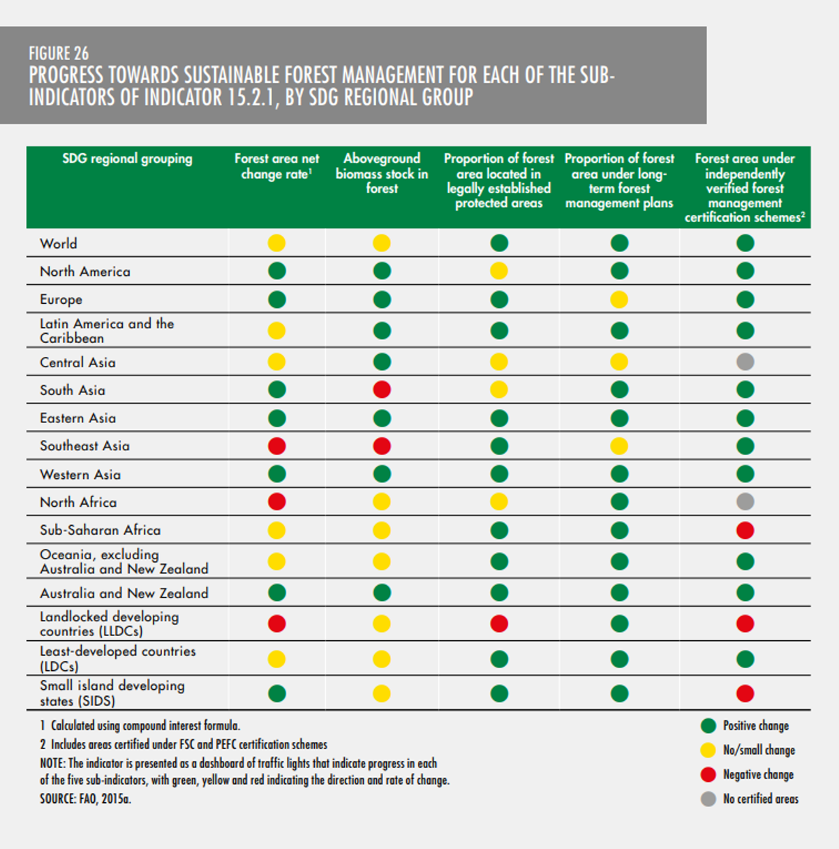
[305] Report: “The State of the World’s Forests 2022: Forest Pathways for Green Recovery and Building Inclusive, Resilient and Sustainable Economies.” United Nations, Food and Agriculture Organization, 2022. <www.fao.org>
Page 7:
According to the definition used in FAO’s [United Nations Food and Agriculture Organization] Global Forest Resources Assessment (FRA), deforestation is “the conversion of forest to other land use independently of whether human-induced or not”.2 That is, deforestation is essentially referring to a change in land use, not in tree cover. Defining deforestation thus implies a definition of forest, which, in the FRA, combines physical criteria (minimum thresholds of 10 percent canopy cover, 0.5 [1.2 acres] ha in area and 5 m [16.4 feet] in height) and a notion of the predominant land use, excluding tree-covered areas where the predominant use is agriculture or urban; hence, the definition excludes plantations of agricultural tree crops (such as oil-palm plantations and orchards) as well as urban parks but includes various types of planted forests (including rubber plantations).3 Nevertheless, many technical and scientific studies do not use FAO’s definition but rather equate deforestation with tree-cover loss without taking land-use criteria into account. This approximation is used in remote-sensing-based methodologies for two reasons – it considers all tree cover (including tree-covered areas not meeting FAO’s forest definition); and it counts instances of non-permanent tree-cover loss (e.g. the clearfelling of a natural or planted forest that will later regrow, and the temporary consequences of a forest fire) as deforestation. When interpreting deforestation figures in different studies, therefore, users should be aware of the impacts of the definitions and tools used. …
Other wooded land. Worldwide, the area of other wooded land was estimated at 977 million ha in 2020, which was 7 percent of the total land area (and about one-quarter the area of the global forest area). …
Recent estimates based on FAO’s latest remote sensing survey suggest that the global area of other wooded land may be significantly higher than reported to FRA 2020.5
Other land with tree cover. Other land with tree cover has four subcategories: 1) trees in urban settings; 2) tree orchards; 3) palms; and 4) agroforestry (Figure 2). The area of palms more than doubled between 1990 and 2020, from 4.2 million ha to 9.3 million ha, based on the 83 countries that reported. Seventy-one countries and territories worldwide reported a total area of 45.4 million ha of agroforestry in 2020, mostly in Asia (31.2 million ha) and Africa (12.8 million ha) (there was also an estimated 1.28 million ha of agroforestry in North and Central America). In the 54 countries and territories that reported trend data on agroforestry, the area of land subject to this use increased by 4.21 million ha between 1990 and 2020, to 43.3 million ha. Most of the increase was in Asia and Africa.6 Note, however, that estimates based on FAO’s latest remote sensing survey suggest that the global area of other land with tree cover may be significantly higher than reported to FRA 2020.
[306] Report: “Global Forest Resources Assessment 2020: Terms and Definitions.” United Nations, Food and Agriculture Organization, February 14, 2018. <www.fao.org>
Page 4:
Forest
Land spanning more than 0.5 hectares with trees higher than 5 meters and a canopy cover of more than 10 percent, or trees able to reach these thresholds in situ [situated in the original place]. It does not include land that is predominantly under agricultural or urban land use.
Explanatory notes
1. Forest is determined both by the presence of trees and the absence of other predominant land uses. The trees should be able to reach a minimum height of 5 meters in situ.
2. Includes areas with young trees that have not yet reached but which are expected to reach a canopy cover of 10 percent and tree height of 5 meters. It also includes areas that are temporarily unstocked due to clear-cutting as part of a forest management practice or natural disasters, and which are expected to be regenerated within 5 years. Local conditions may, in exceptional cases, justify that a longer time frame is used.
3. Includes forest roads, firebreaks and other small open areas; forest in national parks, nature reserves and other protected areas such as those of specific environmental, scientific, historical, cultural or spiritual interest.
4. Includes windbreaks, shelterbelts and corridors of trees with an area of more than 0.5 hectares and width of more than 20 meters.
5. Includes abandoned shifting cultivation land with a regeneration of trees that have, or are expected to reach, a canopy cover of 10 percent and tree height of 5 meters.
6. Includes areas with mangroves in tidal zones, regardless whether this area is classified as land area or not.
7. Includes rubber-wood, cork oak and Christmas tree plantations.
8. Includes areas with bamboo and palms provided that land use, height and canopy cover criteria are met.
9. Includes areas outside the legally designated forest land which meet the definition of “forest”.
10. Excludes tree stands in agricultural production systems, such as fruit tree plantations, oil palm plantations, olive orchards and agroforestry systems when crops are grown under tree cover. Note: Some agroforestry systems such as the “Taungya” system where crops are grown only during the first years of the forest rotation should be classified as forest.
[307] Calculated with data from the paper: “Global Land Change From 1982 to 2016.” By Xiao-Peng Song and others. Nature, August 30, 2018. Pages 639–651. <www.nature.com>
Page 639:
Land change is a cause and consequence of global environmental change.1,2 Changes in land use and land cover considerably alter the Earth’s energy balance and biogeochemical cycles, which contributes to climate change and—in turn—affects land surface properties and the provision of ecosystem services.1–4 However, quantification of global land change is lacking. Here we analyse 35 years’ worth of satellite data and provide a comprehensive record of global land-change dynamics during the period 1982–2016. We show that—contrary to the prevailing view that forest area has declined globally5—tree cover has increased by 2.24 million km2 (+7.1% relative to the 1982 level). This overall net gain is the result of a net loss in the tropics being outweighed by a net gain in the extratropics.
The total area of tree cover increased by 2.24 million km2 from 1982 to 2016 (90% confidence interval (CI): 0.93, 3.42 million km2), which represents a +7.1% change relative to 1982 tree cover….
Page 650: “Extended Data Table 1. Estimates of 1982 Land-Cover Area and 1982–2016 Land-Cover Change at Continental and Global Scales … Tree Canopy Cover … Area 1982 (103 km2) … Global [=] 31,628”
CALCULATIONS:
[308] Article: “How It Might Be: Species.” By Sandra Henderson. EPA Journal, January/February 1989. Pages 21–22. <nepis.epa.gov>
Page 21:
Grizzly bears, elk, peregrine falcons, California condors, rainbow trout, monarch butterflies: the inventory of species that provide beauty and function in our ecosystems seems endless. Yet scientists are warning of a possible loss of 20 percent of the earth’s species before the end of the century—a rate of species destruction greater than any since the mass extinctions of the dinosaurs 65 million years ago.
A major factor in this modern species extinction may be our alteration of the earth’s climate: global warming due to increased concentrations of greenhouse gases. As a result of the Greenhouse Effect, animal life is likely to be affected by several processes: shifting climatic zones. changes in vegetation zones, rising sea level, and increased frequency of natural catastrophic events.
Page 22: “Henderson is a biogeographer at EPA’s Environmental Research Laboratory in Corvallis, Oregon.”
[309] Paper: “How Many Species Are There on Earth and in the Ocean?” By Camilo Mora and others. PLoS Biology, August 23, 2011. <journals.plos.org>
Abstract:
The diversity of life is one of the most striking aspects of our planet; hence knowing how many species inhabit Earth is among the most fundamental questions in science. Yet the answer to this question remains enigmatic, as efforts to sample the world’s biodiversity to date have been limited and thus have precluded direct quantification of global species richness, and because indirect estimates rely on assumptions that have proven highly controversial. Here we show that the higher taxonomic classification of species (i.e., the assignment of species to phylum, class, order, family, and genus) follows a consistent and predictable pattern from which the total number of species in a taxonomic group can be estimated. This approach was validated against well-known taxa, and when applied to all domains of life, it predicts ∼8.7 million (±1.3 million SE) eukaryotic species globally, of which ∼2.2 million (±0.18 million SE) are marine. In spite of 250 years of taxonomic classification and over 1.2 million species already catalogued in a central database, our results suggest that some 86% of existing species on Earth and 91% of species in the ocean still await description.
[310] CALCULATION: 1,200,000 × 0.2 = 240,000
[311] Book: 2004 IUCN Red List of Threatened Species: A Global Species Assessment. Edited by Jonathan E.M. Baillie, Craig Hilton-Taylor, and Simon N. Stuart. World Conservation Union, 2004. <portals.iucn.org>
Page 46:
At least 27 species are recorded as having become Extinct or Extinct in the Wild during the last 20 years (1984–2004) (Tables 3.2 and 3.3). Inherent in identifying very recent extinctions is the problem of extinctions not being included because they are not yet confirmed. For example, eight species of birds are thought to have become Extinct or Extinct in the Wild over the past 20 years, but they are not included, as further research is needed prove the last individual has died (Box 3.2).
[312] Paper: “Historical Bird and Terrestrial Mammal Extinction Rates and Causes.” By Craig Loehle and Willis Eschenbach. Diversity and Distributions, October 13, 2011. Pages 84–91. <onlinelibrary.wiley.com>
Page 84: “Only six continental birds and three continental mammals were recorded in standard databases as going extinct since 1500 compared to 123 bird species and 58 mammal species on islands.”
Page 87:
We can also evaluate continental extinction rates relative to the species pool. The three extinct mammals represent approximately 0.08% of the continental species pool. Even if we assume that all three went extinct in the past 100 years (vs. 500 years), it would take, at this rate, 1,235 years for 1% of continental mammals to go extinct. Similarly for birds, the six species represent 0.062% of the 9,672 species pool and it would take 1,613 years to lose 1% of extant species at current rates even if the recorded extinctions all took place over the last 100 years.
Page 88:
Habitat loss has, of course, played a role in the extinction of some continental species. However, it is worth noting that to date, no continental mammal or bird in our databases has been documented to have gone extinct solely because of habitat reduction. …
Our results do not support statements or projections by others of grossly elevated extinction rates for continental bird and mammal fauna over the last 500 years compared with background rates.
[313] Paper: “Marine Defaunation: Animal Loss in the Global Ocean.” By Douglas J. McCauley and others. Science, January 16, 2015. Pages 1255641-1–1255641-7. <www.sciencemag.org>
Page 1255641-1: “The International Union for Conservation of Nature (IUCN) records only 15 global extinctions of marine animal species in the past 514 years (i.e., limit of IUCN temporal coverage) and none in the past five decades.8, 9”
NOTE: The paper projects that mankind is going to cause “a major extinction” of marine animals. This article from Just Facts shows how that forecast is based on misleading claims and is inconsistent with the documented facts of this matter.
[314] Article: “The Cooling World.” By Peter Gwynne. Newsweek, April 28, 1975. <www.washingtontimes.com>
The Cooling World
There are ominous signs that the Earth’s weather patterns have begun to change dramatically and that these changes may portend a drastic decline in food production—with serious political implications for just about every nation on Earth. The drop in food output could begin quite soon, perhaps only 10 years from now. …
The evidence in support of these predictions has now begun to accumulate so massively that meteorologists are hard-pressed to keep up with it. …
… Meteorologists disagree about the cause and extent of the trend, as well as over its specific impact on local weather conditions. But they are almost unanimous in the view that the trend will reduce agricultural productivity for the rest of the century. …
Climatologists are pessimistic that political leaders will take any positive action to compensate for the climatic change, or even to allay its effects. … The longer the planners delay, the more difficult will they find it to cope with climatic change once the results become grim reality.
[315] Calculated with data from the report: “World Agriculture: Towards 2015/2030 – An FAO Perspective.” Edited by Jelle Bruinsma. Food and Agriculture Organization of the United Nations, 2003. <www.fao.org>
Page 29:
Food consumption, in terms of kcal/person/day,† is the key variable used for measuring and evaluating the evolution of the world food situation.1 The world has made significant progress in raising food consumption per person. It increased from an average of 2,360 kcal/person/day in the mid-1960s to 2,800 kcal/person/day currently (Table 2.1). This growth was accompanied by significant structural change. Diets shifted towards more livestock products, vegetable oils, etc. and away from staples such as roots and tubers (Tables 2.7, 2.8). The increase in world average kcal/person/ day would have been even higher but for the declines in the transition economies in the 1990s.
1 The more correct term for this variable would be “national average apparent food consumption,” since the data come from the national food balance sheets rather than from consumption surveys. The term “food consumption” is used in this sense here and in other chapters.
Data extracted from pages 30–31:
Table 2.1. Per capita food consumption (kcal/person/day) …
Figure 2.1. Per capita food consumption, developing countries with over 100 million population in 1997/99 …
Table 2.2. Population Living in Countries with Given Per Capita Food Consumption
|
Year |
Food Consumption (kcal/person/day) |
Population (millions) |
||
|
World |
Developing Countries |
China |
World |
|
|
1974/76 |
2,435 |
2,152 |
< 2,200 |
4,053 |
|
1997/99 |
2,803 |
2,681 |
> 3,000 |
5,878 |
|
Increase‡ |
15.10% |
24.60% |
> 36.4% |
45.00% |
NOTES:
[316] Calculated with the dataset: “Atmospheric Carbon Dioxide Record from the South Pole.” By R.F. Keeling and others, 2008. Data provided in “Trends: A Compendium of Data on Global Change” by the U.S. Department of Energy, Oak Ridge National Laboratory, Carbon Dioxide Information Analysis Center. <cdiac.ess-dive.lbl.gov>
NOTES:
[317] Calculated with:
a) Dataset: “Land-Ocean: Global Means.” NASA, Goddard Institute for Space Studies. Accessed May 4, 2023 at <data.giss.nasa.gov>
b) Webpage: “GISS Surface Temperature Analysis (GISTEMP v4).” NASA, Goddard Institute for Space Studies. Accessed May 4, 2023 at <data.giss.nasa.gov>
“The GISS [Goddard Institute for Space Studies] Surface Temperature Analysis (GISTEMP v4) is an estimate of global surface temperature change. … The following are … temperature anomalies, i.e. deviations from the corresponding 1951–1980 means.”
NOTE: An Excel file containing the data and calculations is available upon request.
[318] Article: “Growth Is Not Enough.” By George Wehrfritz. Newsweek, April 29, 2007. <www.newsweek.com>
“Similarly, China’s toxic rivers, smog, mass migrations and serious food shortages due to global warming all suggest that Asia’s ‘grow first, clean up later’ mentality is out of step with the gravity of the environmental challenge the region as a whole now faces.”
[319] Article: “McKinsey: Cutting Carbon Won’t Cost Much.” By Diana Farrell. Newsweek, November 14, 2008. <www.newsweek.com>
“Likewise, to avoid the potential nightmares of global warming, such as mass migrations from flooded cities and starvation due to drought, the scientific consensus is we need to cut carbon emissions by at least 50 percent from 1990 levels by 2050.”
[320] Dataset: “Prevalence of Undernourishment (% of Population).” World Bank, March 21, 2023. Accessed May 9, 2023 at <data.worldbank.org>
Prevalence of undernourishments is the percentage of the population whose habitual food consumption is insufficient to provide the dietary energy levels that are required to maintain a normal active and healthy life. Data showing as 2.5 may signify a prevalence of undernourishment below 2.5% …
Limitations and Exceptions: From a policy and program standpoint, this measure has its limits. First, food insecurity exists even where food availability is not a problem because of inadequate access of poor households to food. Second, food insecurity is an individual or household phenomenon, and the average food available to each person, even corrected for possible effects of low income, is not a good predictor of food insecurity among the population. And third, nutrition security is determined not only by food security but also by the quality of care of mothers and children and the quality of the household’s health environment (Smith and Haddad 2000). …
Statistical Concept and Methodology: Data on undernourishment are from the Food and Agriculture Organization (FAO) of the United Nations and measure food deprivation based on average food available for human consumption per person, the level of inequality in access to food, and the minimum calories required for an average person.
NOTE: In 2021, the UN Food and Agriculture Organization changed its methodology for measuring undernourishment, resulting in significantly different results. The next three footnotes document the previous data and the reason for the UN’s changes.
[321] Dataset: “Food Security Indicators.” United Nations Food and Agriculture Organization, October 9, 2019. <www.fao.org>
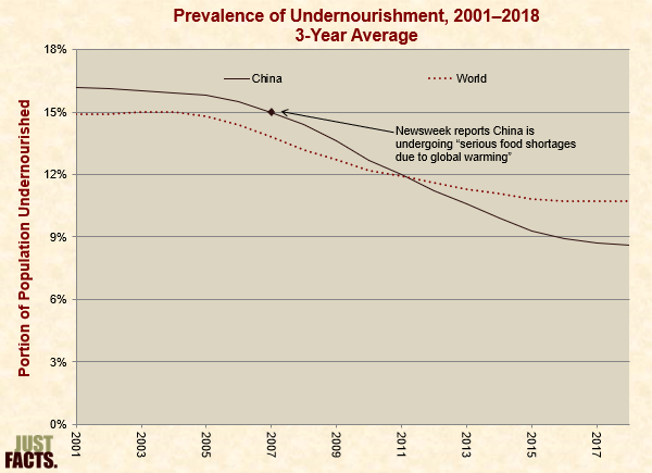
[322] Report: “The State of Food Security and Nutrition in the World: Transforming Food Systems for Affordable Healthy Diets.” United Nations Food and Agriculture Organization, October 5, 2020. Updated 10/15/21. <www.fao.org>
Pages 5–7:
Updated Information for China Improves the Accuracy of Global Hunger Estimates
Revising parameters to estimate the PoU [Prevalence of Undernourishment] is standard procedure, conducted annually as more data become available. … This year has been rich in updates, including revision of the crucial parameter of inequality in food consumption for 13 countries, among them some of the world’s most populous. As highlighted in previous editions, particularly problematic until this year had been access to more recent data to revise the parameter of inequality in food consumption for China. …
This year FAO [Food and Agriculture Organization] obtained data from two surveys in China that could be used to update the PoU estimates. The first is the China Health and Nutrition Survey (CHNS)** conducted from 1990 to 2011, covering 12 provincial-level administrative regions of China. The second is the China Household Finance Survey (CHFS),*** which covers 28 out of 34 provincial-level administrative regions of China, and was conducted every two years from 2011 to 2017. With these data it was possible to update the information on inequality of dietary energy consumption across the Chinese population and, consequently, the estimates of the PoU for China, and to revise the whole series back to 2000 for consistency. …
The result was a substantial downward shift of the entire series of global hunger numbers, as depicted in Figure A. …
** CHNS is collected by the National Institute for Nutrition and Health (NINH), former National Institute of Nutrition and Food Safety, at the Chinese Center for Disease Control and Prevention (CCDC) and the Carolina Population Center at the University of North Carolina at Chapel Hill.
*** CHFS is collected by the Survey and Research Center for China Household Finance of the Research Institute of Economics and Management at the Southwestern University of Finance and Economics in Chengdu, Sichuan, China.
Page 13:
As this process usually implies backward revisions of the entire series, readers must avoid comparing PoU series across different editions of this report. They should always refer to the most current report, including for past values. This is especially important this year, given the significant downward revision of the series of PoU estimates resulting from the updated PoU for China….
[323] Working paper: “Methodological Note on New Estimates of the Prevalence of Undernourishment in China.” By Carlo Cafiero, Juan Feng, and Adeeba Ishaq. Food and Agriculture Organization of the United Nations, July 17, 2020. <www.fao.org>
Pages 1–2:
The Food and Agriculture Organization of the United Nations (FAO) estimates the prevalence of undernourishment (PoU) in all countries and regions of the world by assuming a probabilistic model for the distribution of the per capita levels of habitual dietary energy consumption in the population. The distribution is characterized in terms of the average (the mean dietary energy consumption in the population) and the coefficient of variation (CV, which is a measure of inequality in food consumption level within the population). As differences in observed food consumption of different people may also reflect differences in dietary energy requirement due to sex, age, body mass and physical activity levels, the key parameter to determine the extent of undernourishment is the coefficient of variation (CV|y) that can be traced back to differences in the households’ socio-economic characteristics that are independent of sex, age, body mass and physical activity of their members.
For mainland China, the last time the CV|y was estimated directly from official survey data was in 1999, in preparation for the first edition of The State of Food Insecurity in the World (SOFI) report. Later, lack of access to the needed data prevented updates and the parameter has been kept constant since then. As a result, FAO’s current assessments of the PoU for China do not reflect possible changes in food consumption inequality within its population since 1999, and therefore may be inaccurate. Such changes may have occurred as a consequence of the likely increases in the levels of dietary energy intake for the poorer strata of the Chinese population due to the rapid, intense economic growth in the country over the last two and a half decades. …
To pursue such strategy, we use data from the China Household Finance Survey (CHFS – a fuller description is provided further below), which covers 28 provinces and municipalities with samples that are designed to be representative of the population of mainland China and is available for the years 2011, 2013, 2015 and 2017. The data are used to estimate average monthly food expenditures for households belonging to different income decile groups. By contrasting these to the findings from the analysis of the CHNS [China Health and Nutrition Survey] data, we empirically validate the relation that exists between average food expenditure and average dietary energy consumption in 2011 and use it to predict average dietary energy consumption levels by income decile in China. These predictions are used to estimate the CV|y in 2013, 2015 and 2017, which is in turn used to update the estimates of the PoU.
Page 8:
Our strategy is to link habitual food consumption, measured in terms of equivalent dietary energy intake, to average monthly food expenditure, measured in real monetary terms, for the provinces and income deciles where it is possible to characterize both variables, and then to exploit data on food expenditure available for all provinces and income deciles from the CHFS to predict the average apparent dietary energy consumption by income decile in the provinces not covered by the CHNS in 2011, and in all provinces of mainland China in 2013, 2015 and 2017.
Equipped with this relationship, we predict levels of DEC [dietary energy consumption] for all income decile groups in all the provinces and years (2011, 2013, 2015 and 2017) for which the CHFS provides data on FOOD_EXP [food expenditures].
Page 13:
Figure 4 Prevalence of undernourishment in mainland China, before and after the revision of the CV|y
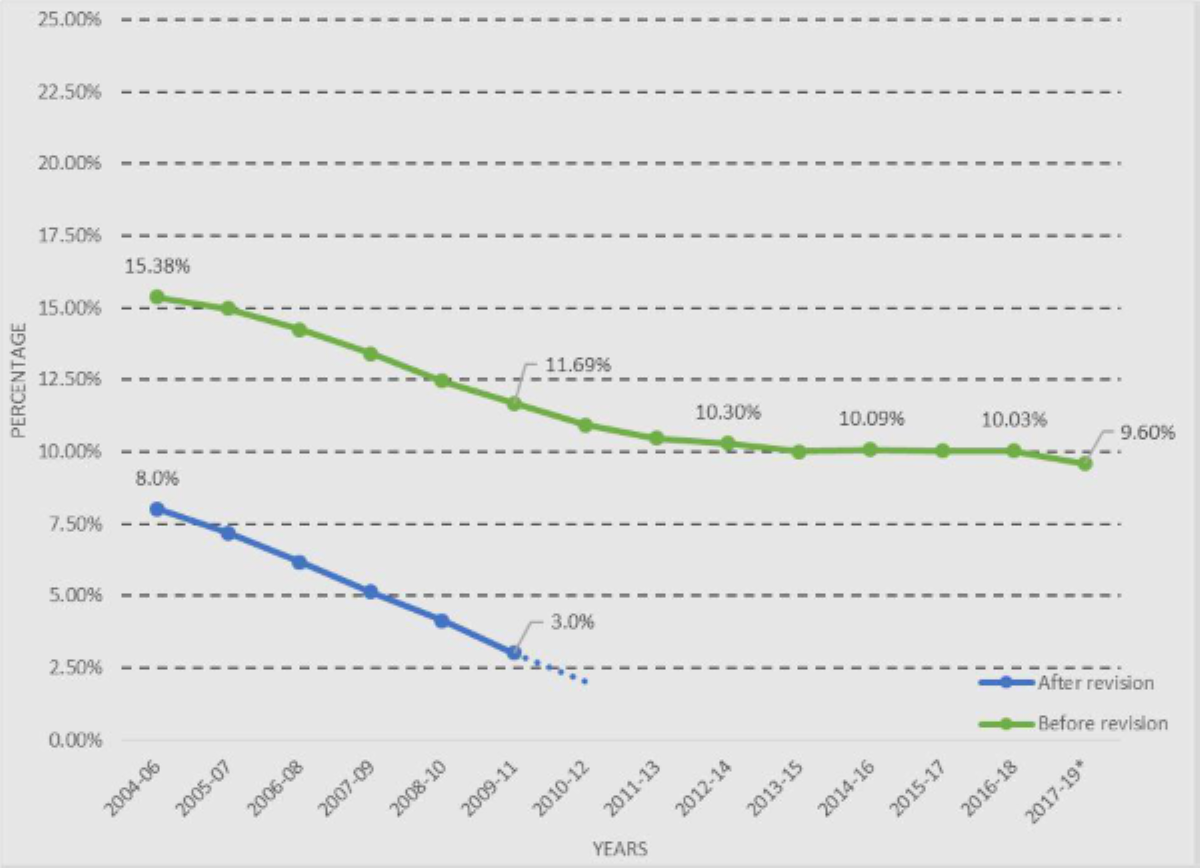
[324] Dataset: “Depth of the Food Deficit (Kilocalories Per Person Per Day).” World Bank, June 28, 2018. <data.worldbank.org>
The depth of the food deficit indicates how many calories would be needed to lift the undernourished from their status, everything else being constant. The average intensity of food deprivation of the undernourished, estimated as the difference between the average dietary energy requirement and the average dietary energy consumption of the undernourished population (food-deprived), is multiplied by the number of undernourished to provide an estimate of the total food deficit in the country, which is then normalized by the total population.
Source: Food and Agriculture Organization, Food Security Statistics. …
Aggregation Method: Weighted average
Development Relevance: The prevalence of undernourishment indicator provides only a partial picture of the food security situation. Recognizing this, FAO [Food and Agriculture Organization of the United Nations] has compiled a preliminary set of food security indicators, available for most countries and years, to contribute to a more comprehensive assessment of the multiple dimensions and manifestations of food insecurity and to effective policies for more effective interventions and responses.
Long Definition: The depth of the food deficit indicates how many calories would be needed to lift the undernourished from their status, everything else being constant. The average intensity of food deprivation of the undernourished, estimated as the difference between the average dietary energy requirement and the average dietary energy consumption of the undernourished population (food-deprived), is multiplied by the number of undernourished to provide an estimate of the total food deficit in the country, which is then normalized by the total population.
Periodicity: Annual
Statistical Concept and Methodology: The indicator is calculated as an average over 3 years.
NOTES: As of May 2023, this is the latest available data from the World Bank or the Food and Agriculture Organization.
[325] Article: “With a Global Focus.” By William H. Mansfield III. EPA Journal, January/February 1989. Pages 37–39. <nepis.epa.gov>
Page 37:
“Global warming may be the greatest challenge facing humankind,” according to Dr. Mostafa K. Tolba, Executive Director of the United Nations Environmental Programme (UNEP) and Under Secretary General of the United Nations. Indeed, the mounting concern about climate change impacts has sent storm warning flags aloft in the United Nations….
Food supplies and forests would be adversely affected. Changes in rainfall patterns would disrupt agriculture. Warmer temperatures would shift grain-growing regions polewards. …
… The natural systems—both plant and animal—will be less able than man to cope and adapt. Any change of temperature, rainfall, and sea level of the magnitude now anticipated will be destructive to natural systems and living things and hence to man as well.
Page 39: “Mansfield is Deputy Executive Director of the United Nations Environment Programme.
[326] Report: “The Future of Food and Agriculture: Trends and Challenges.” United Nations, Food and Agriculture Organization, 2017. <www.fao.org>
Page 85:
With the increases in food supply in recent decades, the world now produces more than enough food to satisfy the dietary needs of the entire global population. The average DES [dietary energy supply] per person per day in low- and middle-income countries is around 2,750 kilocalories and in high-income countries it is around 3,350 kilocalories. Both these figures exceed the minimum requirement of around 1,950 kilocalories per person per day….6 The same applies to protein requirements.7
However, adequate food availability does not automatically imply adequate food intake by all. First, inequality in incomes and other means of subsistence explain large differences in access to food and why still hundreds of millions of people are undernourished. Second, poorer households tend to face impediments to the adequate utilization of food owing to lack of access to facilities, such as food storage, cooking equipment and clean water, and to services, such as health care and basic nutrition education. Third, the dietary transition is partially reflected in improved access to more nutritious foods, including meat, dairy products, fruits and vegetables, but not necessary in the right balance. Analyses based on household surveys, as well as the trends shown above based on the FAO [Food and Agriculture Organization] food balance sheets, suggest accelerated growth in consumption of meat and slower growth in consumption of fruits and vegetables.8 This trend, together with rapidly growing consumption of processed foods, often with excessive quantities of salt, sugar, and preservatives, has given rise to concerns over the shift towards less healthy diets and the increasing prevalence of micronutrient deficiency and overweight.
[327] Constructed with the report: “Statistical Yearbook: World Food and Agriculture 2022.” Food and Agricultural Organization of the United Nations, 2022. <www.fao.org>
Page 275: “Table 42. Average Dietary Energy Supply (kcal per capita per day)”
[328] Paper: “Low Sea Level Rise Projections From Mountain Glaciers and Icecaps Under Global Warming.” By Sarah C. B. Raper and Roger J. Braithwaite. Nature, January 16, 2006. <www.nature.com>
“The largest contributions to sea level rise are estimated to come from thermal expansion (0.288 m) and the melting of mountain glaciers and icecaps (0.106 m), with smaller inputs from Greenland (0.024 m) and Antarctica (–0.074 m).1”
[329] Paper: “Recent Loss of Floating Ice and the Consequent Sea Level Contribution.” By Andrew Shepherd and others. Geophysical Research Letters, July 2010. <discovery.ucl.ac.uk>
Page 1:
Altogether, 746 ± 127 km3 yr−1 of floating ice was lost between 1994 and 2004, a value that exceeds considerably the reduction in grounded ice over the same period. Although the losses are equivalent to a small (49 ± 8 μm yr−1) rise in mean sea level….
The melting of floating ice contributes to the rate at which global sea level changes due to differences in the density and temperature of fresh- and sea-water [Jenkins and Holland, 2007]. If ice is added to an ocean, there is an initial rise in sea level equal to the volume of displaced water. As the ice melts, the ocean freshens and cools and, according to the rates at which these opposing processes take place, a concommital change in ocean volume occurs.
Page 4: “Today, the steric change in global sea level associated with trends in floating ice mass amounts to just 1.6% of the measured rate of sea level rise (3.1 ± 0.7 mm yr−1 [Bindoff and others, 2007] and is considerably smaller than contributions due to other components of the cryosphere [Lemke and others, 2007] or thermal expansion of the oceans [Bindoff and others, 2007].”
[330] For the reason described in the New York Times article below, it is commonly believed that melting sea ice does not contribute to sea level changes, but as explained in the footnote above, melting sea ice can influence sea level “due to differences in the density and temperature of fresh- and sea-water.” However, at the current estimated rate (49 ± 8 μm yr−1), it would take 446 to 620 years for this phenomena to raise sea level by one inch.
CALCULATIONS:
Article: “Frozen Key to Our Climate: The World’s Ice Masses May Be Ushering in a Fifth Ice Age.” By Leonard Engel. New York Times, December 7, 1958. <www.nytimes.com>
[T]he break-up of the floating Artic ice … would not alter sea levels by a single millimeter because, when floating ice melts, it takes up only the space formerly occupied by its submerged part. (A simple demonstration proves this: Put ice cubes in a glass until they reach little higher than the brim, then fill the glass with water exactly to the brim. There will be no change in water level and no overflow as the ice melts.)
[331] Article: “The Uncertainties of Global Warming: Sea Level Could Rise in South, Fall in North.” By Gerald Traufette (translated from the German by Christopher Sultan). Der Spiegel, December 2, 2010. <www.spiegel.de>
Stammer, who is the director of the Center for Marine and Climate Research at the University of Hamburg, is familiar with the incorrect notions that lay people have, which is why he likes to present them with two numbers to shatter their illusions. “In the Indian Ocean, the sea level is about 100 meters (330 feet) below the average, while the waters around Iceland are 60 meters above the average.” …
… Regional effects, on the other hand, are partly influenced by winds and currents, with gravity and the laws of thermodynamics also playing an important role. …
… [I]n late December 1992 … a satellite was placed into service that uses a radar altimeter to measure the sea level, to within a few centimeters, anywhere in the oceans. …
… [W]hile seas have risen by about 15 centimeters [5.9”] in the tropical Western Pacific, the ocean near San Francisco has fallen by about the same amount.”
[332] Paper: “Patterns of Indian Ocean Sea-Level Change in a Warming Climate.” By Weiqing Han and others. Nature Geoscience, July 11, 2010. Pages 546–550. <apps.dtic.mil>
Pages 546–547:
Global sea level has risen during the past decades as a result of thermal expansion of the warming ocean and freshwater addition from melting continental ice.1 However, sea-level rise is not globally uniform.1–5 Regional sea levels can be affected by changes in atmospheric or oceanic circulation. As long-term observational records are scarce, regional changes in sea level in the Indian Ocean are poorly constrained. Yet estimates of future sea-level changes are essential for effective risk assessment.2 Here we combine in situ and satellite observations of Indian Ocean sea level with climate-model simulations, to identify a distinct spatial pattern of sea-level rise since the 1960s. We find that sea level has decreased substantially in the south tropical Indian Ocean whereas it has increased elsewhere. This pattern is driven by changing surface winds associated with a combined invigoration of the Indian Ocean Hadley and Walker cells, patterns of atmospheric overturning circulation in the north–south and east–west direction, respectively, which is partly attributable to rising levels of atmospheric greenhouse gases. We conclude that—if ongoing anthropogenic warming dominates natural variability—the pattern we detected is likely to persist and to increase the environmental stress on some coasts and islands in the Indian Ocean. …
Time series of sea level from HYCOM [Hybrid Coordinate Ocean Model] averaged in four representative regions show persistent trends of sea-level fall and rise, and they are not caused by a jump in 1976/1977 when Pacific climate shift occurred. However, the sea-level fall in region A rebounds over the past decade (Fig. 2). They agree well with satellite altimeter data13 from 1993 to 2008. Sea-level trends for this shorter period do differ markedly from that of 1961 to 2008 (Fig. 2A), as might be expected from natural decadal variability. This is why much longer records are needed to detect anthropogenic sea-level change.14
[333] Paper: “Recent Global Sea Level Acceleration Started Over 200 Years Ago?” By S. Jevrejeva and others. Geophysical Research Letters, April 30, 2008. <onlinelibrary.wiley.com>
Page 1: “We present a reconstruction of global sea level (GSL) since 1700 calculated from tide gauge records and analyse the evolution of global sea level acceleration during the past 300 years.”
[334] Webpage: “Tide Gauge Sea Level.” University of Colorado, Sea Level Research Group. Edited May 17, 2011. <sealevel.colorado.edu>
“Traditionally, global sea level change has been estimated from tide gauge measurements collected over the last century. Tide gauges, usually placed on piers, measure the sea level relative to a nearby geodetic [land-based] benchmark. … Although the global network of tide gauges comprises of a poorly distributed sea level measurement system, it offers the only source of historical, precise, long-term sea level data.”
[335] Paper: “Recent Global Sea Level Acceleration Started Over 200 Years Ago?” By S. Jevrejeva and others. Geophysical Research Letters, April 30, 2008. <onlinelibrary.wiley.com>
Page 1:
We present a reconstruction of global sea level (GSL) since 1700 calculated from tide gauge records and analyse the evolution of global sea level acceleration during the past 300 years. We provide observational evidence that sea level acceleration up to the present … appears to have started at the end of the 18th century. Sea level rose by 6 cm during the 19th century and 19 cm in the 20th century. … All data sets were corrected for local datum changes and glacial isostatic adjustment (GIA) of the solid Earth [Peltier, 2001].
Page 2: “We calculate an acceleration … by fitting a second order polynomial fit to the extended GSL (Figure 1) for the period 1700–2003. The sea level acceleration … appears to have started at the end of the 18th century, although a significant increase does not occur until much later in the 19th century.”
NOTES:
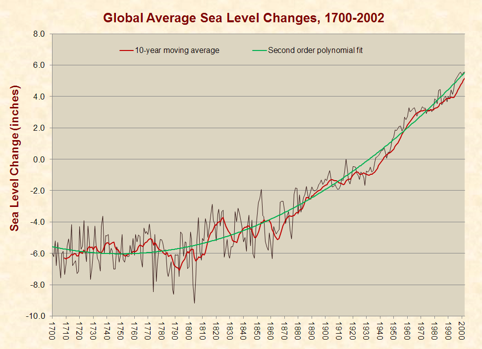
[336] Year surface temperatures began to rise determined with:
a) Dataset: “Land-Ocean: Global Means.” NASA, Goddard Institute for Space Studies. Accessed May 4, 2023 at <data.giss.nasa.gov>
b) Webpage: “GISS Surface Temperature Analysis (GISTEMP v4).” NASA, Goddard Institute for Space Studies. Accessed May 4, 2023 at <data.giss.nasa.gov>
“The GISS [Goddard Institute for Space Studies] Surface Temperature Analysis (GISTEMP v4) is an estimate of global surface temperature change. Graphs and tables are updated around the middle of every month using current data files from NOAA [National Oceanic and Atmospheric Administration] GHCN [Global Historical Climatology Network] v4 (meteorological stations), and ERSST [Extended Reconstructed Sea Surface Temperature] v5 (ocean areas)…. The following are … temperature anomalies, i.e. deviations from the corresponding 1951–1980 means.”
NOTES:
CALCULATION: 1907 (year surface temperatures began to rise) – 1860 (year sea level began to rise) = 47 years
[337] Calculated with data from:
a) The facts above documenting that natural processes emit 770 billion metric tons of CO2 per year.
b) Dataset: “2022 Global Budget 2022 v1.0.” <www.icos-cp.eu>
Tab: “Fossil Emissions by Category … Fossil Fuel and Cement Production Emissions by Fuel Type … All values in million tonnes of carbon per year (MtC/yr) … 1MtC = 1 million tonne of carbon = 3.664 million tonnes of CO2 … MtC/yr … Year … 1956 … Fossil Emissions Excluding Carbonation [=] 2,162.73 [Total fossil emissions include: Coal, Oil, Gas, Cement Emission, Flaring and Other]”
CALCULATIONS:
[338] Calculated with data from the paper: “Sea-Level Acceleration Based on U.S. Tide Gauges and Extensions of Previous Global-Gauge Analyses.” By J.R. Houston and R.G. Dean. Journal of Coastal Research, February 23, 2011. Pages 409–417. <www.jcronline.org>
Page 409:
Without sea-level acceleration, the 20th-century sea-level trend of 1.7 mm/y would produce a rise of only approximately 0.15 m [5.9 in.] from 2010 to 2100.…
In the Fourth Assessment Report (4AR) [2007] of the Intergovernmental Panel on Climate Change (IPCC), Bindoff and others (2007) project a global sea-level rise relative to 1990 of 18–59 cm [7–23 in.] by 2100 and add as much as 0.20 cm† to the upper limit if melting of ice sheets increases in proportion to global average surface temperature increases (Meehl and others, 2007).
† NOTE: This unit was transcribed improperly and should be meters instead of centimeters. Just Facts has notified the authors of the paper about the error.
CALCULATIONS:
[339] Report: “The Ocean and Cryosphere in a Changing Climate.” Edited by Hans-Otto Pörtner and others. Intergovernmental Panel on Climate Change, November 29, 2021. Updated 1/26/2022. <www.ipcc.ch>
Chapter 4: “Sea Level Rise and Implications for Low Lying Islands, Coasts and Communities.” By Michael Oppenheimer and others. Pages 321–445. <www.ipcc.ch>
Page 323:
Global mean sea level (GMSL) is rising (virtually certain1) and accelerating (high confidence2). The sum of glacier and ice sheet contributions is now the dominant source of GMSL rise (very high confidence). GMSL from tide gauges and altimetry observations increased from 1.4 mm yr–1 over the period 1901–1990 to 2.1 mm yr–1 over the period 1970–2015 to 3.2 mm yr–1 over the period 1993–2015 to 3.6 mm yr–1 over the period 2006–2015 (high confidence). The dominant cause of GMSL rise since 1970 is anthropogenic forcing (high confidence)….
Page 324: “SLR [sea level rise] at the end of the century is projected to be faster under all scenarios, including those compatible with achieving the long-term temperature goal set out in the Paris Agreement. GMSL will rise between 0.43 m (0.29–0.59 m, likely range; RCP2.6) and 0.84 m (0.61–1.10 m, likely range; RCP8.5) by 2100 (medium confidence) relative to 1986–2005.”
[340] Report: “Changing Climate and the Coast, Volume 1: Adaptive Responses and Their Economic, Environmental, and Institutional Implications.” Edited by James G. Titus. U.S. Environmental Protection Agency and United Nations Environment Program, May 1990. <nepis.epa.gov>
Page iii:
Increasing concentrations of carbon dioxide and other gases released by human activities are expected to warm the Earth by a mechanism commonly known as the “greenhouse effect.” Such a warming could raise the level of the oceans and thereby inundate low-lying areas, erode beaches, exacerbate coastal flooding, and increase the salinity of estuaries and aquifers. …
… This report presents the findings of a conference held in Miami from November 27 to December 1 on the under the auspices of the Coastal Management Subgroup of the IPCC’s [Intergovernmental Panel on Climate Change’s] Response Strategies Working Group. The Miami conference focused on the implications of sea level rise for Western Africa, the Americas, the Mediterranean Basin, and the rest of Europe; a second conference held in Perth, Australia addressed the other half of the world.
Page 3: “[T]here is a growing consensus among scientists that the atmospheric buildup of greenhouse gases could change global climate and accelerate the rate of sea level rise, which would place further stress on coastal zones. Loss of lives, deterioration of the environment, and undesirable social and economic dislocation may become unavoidable.”
Page 5:
Tidal gauge records show that global sea level has been rising l to 2 millimeters per year over the last century. However, according to IPCC Working Group I, models of the climate, oceans, and cryosphere suggest that sea level could rise 4 to 6 millimeters per year on average through the year 2050 for a total rise of 25 to 40 centimeters. The accelerated rise would be due principally to thermal expansion of the oceans and melting of small mountain glaciers.
[341] Paper: “A 20th Century Acceleration in Global Sea-Level Rise.” By John A. Church and Neil J. White. Geophysical Research Letters, January 6, 2006. <citeseerx.ist.psu.edu>
Page 1:
Multi-century sea-level records and climate models indicate an acceleration of sea-level rise, but no 20th century acceleration has previously been detected. A reconstruction of global sea level using tide-gauge data from 1950 to 2000 indicates a larger rate of rise after 1993 and other periods of rapid sea-level rise but no significant acceleration over this period. Here, we extend the reconstruction of global mean sea level back to 1870 and find a sea-level rise from January 1870 to December 2004 of 195 mm, a 20th century rate of sea-level rise of 1.7 ± 0.3 mm yr-1 [per year] and a significant acceleration of sea-level rise of 0.013 ± 0.006 mm yr–2 [per year squared]. This acceleration is an important confirmation of climate change simulations which show an acceleration not previously observed. If this acceleration remained constant then the 1990 to 2100 rise would range from 280 to 340 mm, consistent with projections in the IPCC TAR [Intergovernmental Panel on Climate Change Third Annual Report, 2007].
[342] Paper: “Sea-Level Acceleration Based on U.S. Tide Gauges and Extensions of Previous Global-Gauge Analyses.” By J.R. Houston and R.G. Dean. Journal of Coastal Research, February 23, 2011. Pages 409–417. <www.jcronline.org>
Page 414:
We analyzed the complete records of 57 U.S. tide gauges that had average record lengths of 82 years and records from 1930 to 2010 for 25 gauges, and we obtained small decelerations of −0.0014 and −0.0123 mm/y2, respectively. We obtained similar decelerations using worldwide-gauge records in the original data set of Church and White (2006) and a 2009 revision (for the periods of 1930–2001 and 1930–2007) and by extending Douglas’s (1992) analyses of worldwide gauges by 25 years.
Page 416: “Our analyses do not indicate acceleration in sea level in U.S. tide gauge records during the 20th century. Instead, for each time period we consider, the records show small decelerations that are consistent with a number of earlier studies of worldwide-gauge records.”
[343] Webpage: “Frequently Asked Questions: What Is the Definition of Global Mean Sea Level (GMSL) and Its Rate?” University of Colorado, Sea Level Research Group. Accessed October 30, 2017 at <sealevel.colorado.edu>
The term “sea level” has many meanings depending upon the context. In satellite altimetry, the measurements are made … relative to the center of the Earth…. Tide gauges, on the other hand, measure sea level relative to the local land surface…. The satellite altimeter estimate of interest is the distance between the sea surface illuminated by the radar altimeter and the center of the Earth…. This distance is estimated by subtracting the measured distance between the satellite and sea surface (after correcting for many effects on the radar signal) from the very precise orbit of the satellite.
[344] Webpage: “Laboratory for Satellite Altimetry / Sea Level Rise.” National Oceanic and Atmospheric Administration, Laboratory for Satellite Altimetry. Last modified March 16, 2020. <www.star.nesdis.noaa.gov>
The measurement of long-term changes in global mean sea level can provide an important corroboration of predictions by climate models of global warming. Satellite altimeter radar measurements can be combined with precisely known spacecraft orbits to measure sea level on a global basis with unprecedented accuracy. A series of satellite missions that started with TOPEX/Poseidon (T/P) in 1992 and continued with Jason-1 (2001–2013), Jason-2 (2008–2019), and Jason-3 (2016–present) estimate global mean sea level every 10 days with an uncertainty of 3–4 mm.
Jason-3, launched 17 January 2016, is a joint effort between NOAA [National Oceanic and Atmospheric Administration], the National Aeronautics and Space Administration, France’s Centre National d’Etudes Spatiales (CNES) and the European Organisation for the Exploitation of Meteorological Satellites (EUMETSAT).
The latest mean sea level time series and maps of regional sea level change can be found on this site.
[345] Calculated with data from:
a) Dataset: “Global Mean Sea Level Time Series (Seasonal Signals Removed), TOPEX and Jason-1, -2, -3.” NOAA Laboratory for Satellite Altimetry. Accessed May 9, 2023 at <www.star.nesdis.noaa.gov>
b) Dataset: “Global Mean Sea Level Time Series (Seasonal Signals Removed), Multiple Altimeters.” NOAA Laboratory for Satellite Altimetry. Accessed May 9, 2023 at <www.star.nesdis.noaa.gov>
NOTES:
[346] Paper: “The Dynamic Response of Reef Islands to Sea Level Rise: Evidence from Multi-Decadal Analysis of Island Change in the Central Pacific.” By Arthur P. Webb and Paul S. Kench. Global and Planetary Change, June 2010. Pages 234–246. <www.sciencedirect.com>
Page 234:
Coral reef islands are low-lying accumulations of unconsolidated, or poorly lithified, carbonate sand and gravel deposited on coral reef platforms by the focusing effect of waves and currents (Stoddart and Steers, 1977). Coral reef islands are commonly found in barrier reef systems (for example Great Barrier Reef); open reef seas (for example Torres Strait) or in mid-ocean atolls. In atoll nations such as Tuvalu, Kiribati and the Maldives reef islands provide the only habitable area, which can carry very high population densities…. These low-lying reef islands and their populations are considered physically vulnerable to a range of climate change impacts including: sea-level rise; changing weather and oceanographic wave regimes, and increased cyclone frequency and intensity (Church and others, 2006; Mimura and others, 2007).
Under current scenarios of global climate-induced sea-level rise of 0.48 to 0.98m [19–39 inches] by 2100 it is widely anticipated that low-lying reef islands will become physically unstable and be unable to support human populations over the coming century (Leatherman, 1997; Connell, 1999). The most anticipated physical impacts of sea-level rise on islands are shoreline erosion, inundation, flooding, salinity intrusion, and reduced resilience of coastal ecosystems (Leatherman, 1997; Mimura, 1999; Khan and others, 2002; Yamano and others, 2007). It is also widely perceived that island erosion will become so widespread that entire atoll nations will disappear rendering their inhabitants among the first environmental refugees of climate change (Connell, 2003, 2004).
[347] Book: Encyclopedia of Coastal Science. Edited by Maurice L. Schwartz. Springer, 2005. Article: “Coral Reef Islands.” By Gisele Muller-Parker. Pages 342–343.
Page 342:
A coral reef island is composed of rocks from coral skeletons, that is, biologically formed calcium carbonate materials derived from the adjacent coral reef and raised above sea level. Coral reef island sizes range from a few square meters to many square kilometers, and they come in all shapes and proportions. Their soils consist of coral fragments, calcareous algae and other limestone detritus [gravel, sand, and silt], varied amount of humus, guano from sea birds, volcanic ash, and drifted pumice (Fosberg, 1976).
Most coral reef islands occur in the Indo-Pacific region. There are over 300 atolls [ring-shaped islands or chains of islands] and extensive barrier reefs in the Pacific ocean and only ten atolls and 2 barrier reefs in the Caribbean region (Milliman, 1973). The total number of coral reef islands is unknown, and varies according to change in sea level and storm activity.
[348] Video: “Tuvalu at Copenhagen: ‘The Fate Of My Country Rests In Your Hands.’ ” December 2009. <www.youtube.com>
[349] Paper: “Patterns of Island Change and Persistence Offer Alternate Adaptation Pathways for Atoll Nations.” By Paul S. Kench and others. Nature Communications, February 9, 2018. <www.nature.com>
Page 2:
Here we present the first comprehensive national-scale analysis of the transformation in physical land resources of the Pacific atoll nation Tuvalu, situated in the central western Pacific…. Comprising 9 atolls and 101 individual reef islands, the nation is home to 10,600 people, 50% of whom are located on the urban island of Fogafale, in Funafuti atoll. We specifically examine spatial differences in island behaviour, of all 101 islands in Tuvalu, over the past four decades (1971–2014), a period in which local sea level has risen at twice the global average…. Surprisingly, we show that all islands have changed and that the dominant mode of change has been island expansion, which has increased the land area of the nation. … [T]otal land area of the nation has expanded by 73.5 ha (2.9%) since 1971.
[350] Paper: “The Dynamic Response of Reef Islands to Sea Level Rise: Evidence from Multi-Decadal Analysis of Island Change in the Central Pacific.” By Arthur P. Webb and Paul S. Kench. Global and Planetary Change, June 2010. Pages 234–246. <www.sciencedirect.com>
Page 234: “Using historical aerial photography and satellite images this study presents the first quantitative analysis of physical changes in 27 atoll islands in the central Pacific over a 19 to 61 yr period. This period of analysis corresponds with instrumental records that show a rate of sea-level rise of 2.0 mm yr−1 in the Pacific….”
Page 241:
The total change in area of reef islands (aggregated for all islands in the study) is an increase in land area of 63 ha [hectares, 1 hectare = 2.47 acres] representing 7% of the total land area of all islands studied. … Forty-three percent of islands have remained relatively stable (<±3% change) over the period of analysis. A further 43% of islands (12 in total) have increased in area by more than 3%. The remaining 15% of islands underwent net reduction in island area of more than 3%.
Of the islands that show a net increase in island area six have increased by more than 10% of their original planform area. … The remaining three islands are in Tarawa atoll with Betio, Bairiki and Nanikai increasing by 30%, 16.3% and 12.5% respectively over the 60 yr period of analysis (Table 2). Of note, the large percentage change on Betio represents an increase of more than 36 ha.
Only one island has shown a net reduction in island area greater than 10%. Tengasu is located on the southwest atoll rim of Funafuti and decreased in area by 14% over the 19 yr period of analysis. However, closer examination of the Tengasu data shows that it was the smallest island in the study sample (0.68 ha) and the absolute change in island area was 0.1 ha, which represents a substantial proportion of the total island area.
Page 245: “Of significance, the results of this study on atoll islands are applicable to islands in other reef settings, as the boundary controls on island formation and change are comparable. Results of this study contradict widespread perceptions that all reef islands are eroding in response to recent sea level rise.”
[351] Article: “U.N. Predicts Disaster if Global Warming Not Checked.” By Peter James Spielmann. Associated Press, June 29, 1989. <www.apnews.com>
A senior U.N. environmental official says entire nations could be wiped off the face of the Earth by rising sea levels if the global warming trend is not reversed by the year 2000.
Coastal flooding and crop failures would create an exodus of “eco-refugees,” threatening political chaos, said Noel Brown, director of the New York office of the U.N. Environment Program, or UNEP.
He said governments have a 10-year window of opportunity to solve the greenhouse effect before it goes beyond human control.
As the warming melts polar icecaps, ocean levels will rise by up to three feet, enough to cover the Maldives and other flat island nations, Brown told The Associated Press in an interview on Wednesday.
[352] Article: “With a Global Focus.” By William H. Mansfield III. EPA Journal, January/February 1989. Pages 37–39. <nepis.epa.gov>
Page 37:
Sea-level rise as a consequence of global warming would immediately threaten that large fraction of the globe living at sea level. Nearly one-third of all human beings live within 36 miles of a coastline. Most of the world’s great seaport cities would be endangered: New Orleans, Amsterdam, Shanghai, Cairo. Some countries—the Maldives Islands in the Indian Ocean, islands in the Pacific—would be inundated. Heavily populated coastal areas such as in Bangladesh and Egypt, where large populations occupy low-lying areas, would suffer extreme dislocation.
Page 39: “Mansfield is Deputy Executive Director of the United Nations Environment Programme.”
[353] Calculated with data from the paper: “Earth’s Surface Water Change Over the Past 30 Years.” By Gennadii Donchyts and others. Nature Climate Change, August 25, 2016. Pages 810–813. <www.nature.com>
Pages 810–811:
Earth’s surface gained 115,000 km2 of water and 173,000 km2 of land over the past 30 years, including 20,135 km2 of water and 33,700 km2 of land in coastal areas. Here, we analyse the gains and losses through the Deltares Aqua Monitor—an open tool that detects land and water changes around the globe. …
The massive growth in satellite data has resulted in a severe demand in storage, computation and smart analytics to enable analysis of planetary-scale data. …
We see that globally, between 1985 and 2015, an area of about 173,000 km2—about the size of Washington State—has been converted to land, and an area of 115,000 km2 has been converted into water.
CALCULATIONS:
[354] Article: “Surface Water Shifting Around the Earth.” By Rebecca Morelle. BBC, August 25. 2016. <www.bbc.com>
[Study coauthor] Dr. Fedor Baart from Deltares said: “We started to look at areas that had not been mapped before.” …
“We expected that the coast would start to retreat due to sea level rise, but the most surprising thing is that the coasts are growing all over the world,” said Dr. Baart.
“We’re [sic] were able to create more land than sea level rise was taking.”
[355] Book: Earth in the Balance: Ecology and the Human Spirit. By Al Gore. Houghton Mifflin, 1992.
Page 73:
About 10 million people in Bangladesh will lose their homes and means of sustenance because of the rising sea level, due to global warming, in the next few decades. Where will they go? Whom will they displace? What political conflicts will result? That is only one example. According to some predictions, not long after Bangladesh feels the impact, up to 60 percent of the present population of Florida may have to be relocated. Where will they go?
[356] Article: “Al Gore Summary.” Encyclopedia Britannica, October 12, 2007. <www.britannica.com>
“Political Affiliation: Democratic Party … He served in the U.S. House of Representatives (1977–85) and later the Senate (1985–93).”
[357] Webpage: “About CEGIS.” Center for Environment and Geographic Information Services. Accessed June 2, 2020 at <www.cegisbd.com>
While Bangladesh is making great strides towards holistic and sustainable development, CEGIS [Center for Environment and Geographic Information Services] has been relentlessly trying since the inception of its predecessor EGIS [Environmental Geographic Information System] in 1995 to support the country’s efforts for sustainable socio-economic development by providing scientific, technological and socio-economic know-how. It is a Public Trust under the Ministry of Water Resources of the Government of Bangladesh.
CEGIS is a scientifically independent organisation and performs integrated environmental analysis using technologies like GIS [geographic information system], RS, IT and databases. It provides solutions to issues and problems in a wide range of sectors, such as—but not limited to—water, land, agriculture, meteorology, forestry, fisheries, morphology, ecology, environment, climate change, archeology, socio-economy, power, transportation and disasters.
[358] Article: “Bangladesh Gaining Land, Not Losing: Scientists.” Agence France-Presse, July 29, 2008. <www.geospatialworld.net>
New data shows that Bangladesh’s landmass is increasing, contradicting forecasts that the South Asian nation will be under the waves by the end of the century, experts say.
Scientists from the Dhaka-based Center for Environment and Geographic Information Services (CEGIS) have studied 32 years of satellite images and say Bangladesh’s landmass has increased by 20 square kilometres (eight square miles) annually.
Maminul Haque Sarker, head of the department at the government-owned centre that looks at boundary changes, told AFP [Agence France-Presse] sediment which travelled down the big Himalayan rivers—the Ganges and the Brahmaputra—had caused the landmass to increase. …
“Satellite images dating back to 1973 and old maps earlier than that show some 1,000 square kilometres of land have risen from the sea,” Sarker said.
[359] Article: “Bangladesh Landmass ‘Is Growing.’ ” By Mark Dummett. BBC News, July 30, 2008. <news.bbc.co.uk>
Satellite images of Bangladesh over the past 32 years show that the country is growing annually by about 20 square kilometres (7.72 square miles), said Maminul Haque Sarker of the Dhaka-based Centre for Environment and Geographic Information Services.
This was due, he said, to the billion tonnes of sediment that the Ganges, the Brahmaputra and 200 other rivers bring from the Himalayas each year before crossing Bangladesh.
[360] Calculated with data from:
a) Report: “Population Trends: Bangladesh.” U.S. Department of Commerce, Economics and Statistics Administration, Bureau of the Census, Center for International Research, March 1993. <www.census.gov>
Page 1: “Bangladesh is the tenth most populous country in the world. Its current estimated population of 119 million is almost one-half the population size of the United States. But its area of 51,703 square miles is only 1.5 percent as large as the area of the United States. Bangladesh has the highest population density (2,310 persons per square mile) among all countries in the world that are not small island nations or city states.”
b) Webpage: “Bangladesh.” World Factbook. U.S. Central Intelligence Agency. Last updated May 1, 2023. <www.cia.gov>
“Population: 167,184,465 (2023 est.)”
CALCULATION: (167 – 119) / 119 = 40.3%
[361] Report: “Florida State of the Coast Report: Preparing for a Sustainable Future.” Florida Department of Community Affairs, Florida Coastal Management Program, September 1996.
Page 6: “In 1990, about 111 million people lived in coastal areas nationwide and Florida accounted for 10.1 million (9%) of those residents.”
[362] Calculated with data from the webpage: “Coastal Population and Housing Search.” National Ocean Economics Program, Middlebury Institute of International Studies at Monterey. Accessed May 10, 2023 at <www.oceaneconomics.org>
|
Florida |
|||
|
Region |
Counties |
Year |
Population |
|
Total |
|||
|
Florida |
All Florida counties |
2021 |
21,781,128 |
|
Shore-adjacent |
All counties |
2021 |
16,283,953 |
CALCULATION: (16,283,953 – 10,100,000) / 10,100,000 = 61%
[363] Webpage: “An Inconvenient Truth.” Participant Media. Accessed June 2, 2020 at <www.participantmedia.com>
From director Davis Guggenheim comes the hit, An Inconvenient Truth, which offers a passionate and inspirational look at one man’s commitment to expose the myths and misconceptions that surround global warming and inspire actions to prevent it. That man is former Vice President Al Gore, who, in the wake of defeat in the 2000 election, re-set the course of his life to focus on an all-out effort to help save the planet from irrevocable change.
[364] Documentary: An Inconvenient Truth. Paramount Pictures, 2006.
NOTE: The sea level rise simulation occurs in a section of the documentary that begins 57 minutes into the film. It is reproduced under the “fair use” provision of U.S. copyright law for “purposes such as criticism” and “comment” (17 U.S.C. §107).
[365] Calculated with data from the paper: “Sea-Level Acceleration Based on U.S. Tide Gauges and Extensions of Previous Global-Gauge Analyses.” By J.R. Houston and R.G. Dean. Journal of Coastal Research, February 23, 2011. Pages 409–417. <www.jcronline.org>
Page 409:
Without sea-level acceleration, the 20th-century sea-level trend of 1.7 mm/y would produce a rise of only approximately 0.15 m [5.9 in.] from 2010 to 2100….
In the Fourth Assessment Report (4AR) [2007] of the Intergovernmental Panel on Climate Change (IPCC), Bindoff and others. (2007) project a global sea-level rise relative to 1990 of 18–59 cm [7–23 in.] by 2100 and add as much as 0.20 cm† to the upper limit if melting of ice sheets increases in proportion to global average surface temperature increases (Meehl and others, 2007).
† NOTE: This unit was transcribed improperly and should be meters instead of centimeters. Just Facts has notified the authors of the paper about the error.
CALCULATIONS:
[366] Article: “Scientists Say Earth’s Warming Could Set Off Wide Disruptions.” By William K. Stevens. New York Times, September 18, 1995. <www.nytimes.com>
A continuing rise in average global sea level, which is likely to amount to more than a foot and a half by the year 2100. [sic] This, say the scientists, would inundate parts of many heavily populated river deltas and the cities on them, making them uninhabitable, and would destroy many beaches around the world. At the most likely rate of rise, some experts say, most of the beaches on the East Coast of the United States would be gone in 25 years. They are already disappearing at an average of 2 to 3 feet a year.
[367] Book: Best Beach Vacations in the Mid-Atlantic: From New York to Washington, D.C. By Donald D. Groff. Macmillan Travel, 1996.
Pages 4–260:
|
New York |
|
|
Montauk |
|
|
1 |
Montauk Town Beach–Kirk Park Beach |
|
2 |
Ditch Plains Beach |
|
3 |
Hither Hills State Park Beach |
|
4 |
Gin Beach |
|
5 |
Fort Pond Bay Beach |
|
East Hamption |
|
|
6 |
Amagansett - Atlantic Avenue Beach |
|
7 |
Amagansett - Indian Wells Beach |
|
8 |
Two Mile Hollow Beach |
|
9 |
Wiborg Beach |
|
10 |
Main Beach |
|
11 |
Georgica Beach |
|
12 |
Bay Beach–Cedar Point Park |
|
Southhampton |
|
|
13 |
Flying Point Beach |
|
14 |
Fowler's Beach |
|
15 |
Old Town Beach |
|
16 |
Wyandanch Lane Beach |
|
17 |
Little Plains Beach |
|
18 |
South Main Street |
|
19 |
Coopers Beach |
|
20 |
Halsey Neck Beach |
|
21 |
Road D |
|
22 |
Dune Beach |
|
23 |
Road G / Shinnecock East County Park |
|
Hampton Bays |
|
|
24 |
Ponquogue Beach |
|
25 |
Road K and Road L–Tiana Beach |
|
26 |
Meschutt Beach County Park |
|
Westhampton |
|
|
27 |
Dolphin Lane Beach |
|
28 |
Hampton Beach |
|
29 |
Rogers Beach |
|
30 |
Westhampton Beach / Lashley Beach |
|
Fire Island |
|
|
31 |
Sailors Haven |
|
32 |
Atlantique Beach |
|
33 |
Saltaire |
|
34 |
Watch Hill |
|
35 |
National Seashore Lighthouse Beach |
|
Robert Moses State Park |
|
|
36 |
Field 2 |
|
37 |
Field 3 |
|
38 |
Field 4 |
|
39 |
Field 5 |
|
Jones Beach State Park |
|
|
40 |
Oceanside |
|
41 |
Zach's Bay |
|
New Jersey |
|
|
Spring Lake |
|
|
42 |
Belmar |
|
43 |
Spring Lake |
|
44 |
Sea Girt |
|
Point Pleasant |
|
|
45 |
Point Pleasant |
|
46 |
Bay Head |
|
47 |
Seaside Heights |
|
48 |
Island Beach State Park |
|
Long Beach Island |
|
|
49 |
Barnegat Light |
|
50 |
Ship Bottom |
|
51 |
Beach Haven |
|
52 |
Holgate |
|
Atlantic City |
|
|
53 |
Main Beach |
|
54 |
East Casino Strip |
|
55 |
Ventnor |
|
56 |
Margate |
|
Ocean City |
|
|
57 |
North End |
|
58 |
South of Music Pier |
|
59 |
South of 21st Street |
|
Sea Isle City |
|
|
60 |
Sea Isle City |
|
61 |
Strathmere |
|
Stone Harbor |
|
|
62 |
Stone Harbor |
|
63 |
Avalon |
|
The Wildwoods |
|
|
64 |
North Wildwood |
|
65 |
Wildwood |
|
66 |
Wildwood Crest |
|
Cape May |
|
|
67 |
City Beaches |
|
68 |
Bay Beach |
|
69 |
East End Beach |
|
70 |
Point Beaches |
|
71 |
Sunset Beach |
|
72 |
Higbee Beach |
|
Delaware |
|
|
Lewes / Cape Henlopen |
|
|
73 |
Beach No. 1 |
|
74 |
Beach No. 2 |
|
75 |
Cape Henlopen State Park Beach |
|
Rehoboth Beach |
|
|
76 |
Rehoboth Beaches |
|
77 |
Cape Henlopen State Park Beach |
|
Dewey Beach |
|
|
78 |
Oceanside |
|
79 |
Bayside |
|
80 |
Tower Road: Oceanside |
|
81 |
Indian River Inlet |
|
Bethany Beach |
|
|
82 |
Bethany Boardwalk Beach |
|
83 |
Fenwick Island State Park |
|
84 |
Fenwick Island |
|
Maryland |
|
|
Ocean City |
|
|
85 |
Ocean City Beach |
|
86 |
Assateague State Park |
|
87 |
North Ocean Beach |
|
88 |
South Ocean Beach |
|
Virginia |
|
|
Chincoteague |
|
|
89 |
Bathhouse No. 1 |
|
90 |
Bathhouse No. 2 |
|
Virginia Beach |
|
|
91 |
Resort Strip Beaches |
|
92 |
Seashore State Park (First Landing) Beach |
|
93 |
Fort Story Beach |
|
94 |
Chesapeake Beach |
|
95 |
Little Island Park |
[368] On June 12, 2023, Just Facts conducted a comprehensive search for each of the beaches listed in the footnote above and found that all of them still exist.
[369] Map: “Mid-Atlantic Coast.” Google Maps, June 12, 2023. <www.google.com>
“U.S. East Coast, north-eastern tip of New York to south-eastern tip of Virginia.”
[370] Search: east coast beaches gone. Google, June 10, 2023. Date delimited to 6/1/1980–6/10/2023. <www.google.com>
[371] Book: Essentials of Meteorology: An Invitation to the Atmosphere (5th edition). By C. Donald Ahrens. Thomson Brooks/Cole, 2008.
Page 470: “Tropical cyclone The general term for storms (cyclones) that form over warm tropical oceans.”
[372] Report: “Science and the Storms: The USGS Response to the Hurricanes of 2005.” Edited by G.S. Farris and others. U.S. Department of the Interior, U.S. Geological Survey, 2007.
Chapter 2, Section “The Major Hurricanes of 2005: A Few Facts.” Compiled by Gaye S. Farris. Pages 12–15. <pubs.usgs.gov>
Page 12:
A cyclone is an atmospheric closed circulation that rotates counterclockwise in the Northern Hemisphere and clockwise in the Southern Hemisphere. A tropical cyclone is a generic name for warm-core, nonfrontal, large-scale, low-pressure cyclones originating over tropical or subtropical waters, with organized deep convection (thunderstorm activity) and a closed surface wind circulation around a well-defined center.
Tropical cyclones include tropical depressions (winds less than 39 mi/hour or 63 km/hour) and tropical storms (39–73 mi/hour or 63–117 km/hour), which receive a name. When tropical cyclone winds reach 74 mi/hour (119 km/hour), they are called one of the following, depending on location:
• hurricanes in the North Atlantic Ocean, the Northeast Pacific Ocean east of the International Dateline, or the South Pacific Ocean east of longitude 160° E
• typhoons in the Northwest Pacific Ocean west of the International Date Line
• severe tropical cyclones in the Southwest Pacific Ocean west of longitude 160° E or Southeast Indian Ocean east of longitude 90° E
• severe cyclonic storms in the North Indian Ocean
• tropical cyclones in the Southwest Indian Ocean
[373] Article: “Global Warming May Spawn More Super-Storms.” By Stephen Leahy.
Inter Press Service News Agency, September 20, 2004. <www.ipsnews.net>
“As the world warms, we expect more and more intense tropical hurricanes and cyclones,” said James McCarthy, a professor of biological oceanography at Harvard University.
Large parts of the world’s oceans are approaching 27 degrees C or warmer during the summer, greatly increasing the odds of major storms, McCarthy told IPS [Inter Press Service].
When water reaches such temperatures, more of it evaporates, priming hurricane or cyclone formation. Once born, a hurricane needs only warm water to build and maintain its strength and intensity.
[374] Webpage: “Global Tropical Cyclone Activity.” Dr. Ryan N. Maue. Updated December 31, 2022. <climatlas.com>
“Figure: Last 50-years+ of Global Tropical Storm and Hurricane frequency – 12-month running sums. The top time series is the number of TCs [tropical cyclones] that reach at least tropical storm strength (maximum lifetime wind speed exceeds 34-knots). The bottom time series is the number of hurricane strength (64-knots+) TCs.”
[375] Report: “Climate Change 2007: The Physical Science Basis.” Edited by S. D. Solomon and others. World Meteorological Organization/United Nations Environment Programme, Intergovernmental Panel on Climate Change. Cambridge University Press, 2007.
Chapter 3: “Observations: Surface and Atmospheric Climate Change.” By Kevin E. Trenberth and others. Pages 235–336. <www.ipcc.ch>
Page 304:
Traditional measures of tropical cyclones, hurricanes and typhoons have varied in different regions of the globe, and typically have required thresholds of estimated wind speed to be crossed for the system to be called a tropical storm, named storm, cyclone, hurricane or typhoon, or major hurricane or super typhoon. Many other measures or terms exist, such as “named storm days”, “hurricane days”, “intense hurricanes”, “net tropical cyclone activity”, and so on.
The ACE [Accumulated Cyclone Energy] index (see Box 3.5), is essentially a wind energy index, defined as the sum of the squares of the estimated six-hour maximum sustained wind speed (knots) for all named systems while they are at least tropical storm strength. Since this index represents a continuous spectrum of both system duration and intensity, it does not suffer as much from the discontinuities inherent in more widely used measures of activity such as the number of tropical storms, hurricanes or major hurricanes. However, the ACE values reported here are not adjusted for known inhomogeneities in the record (discussed below). … Prior to about 1970, there was no satellite imagery to help estimate the intensity and size of tropical storms, so the estimates of ACE are less reliable, and values are not given prior to about the mid- or late 1970s in the Indian Ocean, South Pacific or Australian regions.
Page 305:
While attention has often been focussed simply on the frequency or number of storms, the intensity, size and duration likely matter more. NOAA’s [National Oceanic and Atmospheric Administration] Accumulated Cyclone Energy (ACE) index (Levinson and Waple, 2004) approximates the collective intensity and duration of tropical storms and hurricanes during a given season and is proportional to maximum surface sustained winds squared. The power dissipation of a storm is proportional to the wind speed cubed (Emanuel, 2005a), as the main dissipation is from surface friction and wind stress effects, and is measured by a Power Dissipation Index (PDI). Consequently, the effects of these storms are highly nonlinear and one big storm may have much greater impacts on the environment and climate system than several smaller storms.
[376] Webpage: “Global Tropical Cyclone Activity.” Dr. Ryan N. Maue. Updated November 30, 2022. <climatlas.com>
“Figure: Last 50-years+ of Global and Northern Hemisphere Accumulated Cyclone Energy [ACE]: 24 month running sums. Note that the year indicated represents the value of ACE through the previous 24-months for the Northern Hemisphere (bottom line/gray boxes) and the entire global (top line/blue boxes). The area in between represents the Southern Hemisphere total ACE.”
[377] Article: “Scientific Survey Shows Voters Widely Accept Misinformation Spread by the Media.” By James D. Agresti. Just Facts, January 2, 2020. <www.justfacts.com>
The survey was conducted by Triton Polling & Research, an academic research firm that serves scholars, corporations, and political campaigns. The responses were obtained through live telephone surveys of 700 likely voters across the U.S. during December 2–11, 2019. This sample size is large enough to accurately represent the U.S. population. Likely voters are people who say they vote “every time there is an opportunity” or in “most” elections.
The margin of sampling error for the total pool of respondents is ±4% with at least 95% confidence. The margins of error for the subsets are 6% for Democrat voters, 6% for Trump voters, 5% for males, 5% for females, 12% for 18 to 34 year olds, 5% for 35 to 64 year olds, and 6% for 65+ year olds.
The survey results presented in this article are slightly weighted to match the ages and genders of likely voters. The political parties and geographic locations of the survey respondents almost precisely match the population of likely voters. Thus, there is no need for weighting based upon these variables.
[378] Dataset: “Just Facts 2019 U.S. Nationwide Survey.” Just Facts, December 2019. <www.justfacts.com>
Page 3:
Q13. Again, thinking about the whole planet, do you think the number and intensity of hurricanes and tropical storms have generally increased since the 1980s?
Yes [=] 63.5%
No [=] 31.8%
Unsure [=] 4.2%
[379] For facts about how surveys work and why some are accurate while others are not, click here.
[380] Article: “A Character Sketch of Greenhouse.” By David Rind. EPA Journal, January/February 1989. Pages 4–7. <nepis.epa.gov>
Page 6: “The GISS [Goddard Institute for Space Studies] model’s forecast for the next 50 years gives changes of 2º C (3.6º F) by the year 2020, which would make the earth warmer than it is thought to have been at any point in historical time. … Rainfall patterns would likely be substantially altered, posing the threat of large-scale disruptions of agricultural and economic productivity, and water shortages in some areas.”
Page 7: “Dr. Rind is an atmospheric scientist at the Institute for Space Studies, Goddard Space Flight Center, National Aeronautics and Space Administration, and an adjunct associate professor at Columbia University. He is a leading researcher on aspects of the greenhouse theory of atmospheric warming from certain gases.”
[381] Article: “Harvey Is What Climate Change Looks Like.” By Eric Holthaus. Politico, August 28, 2017. <www.politico.com>
Climate change is making rainstorms everywhere worse, but particularly on the Gulf Coast. Since the 1950s, Houston has seen a 167 percent increase in the frequency of the most intense downpours. …
Eric Holthaus is a meteorologist and contributing writer for Grist.
[382] Article: “Global Warming Is Increasing Rainfall Rates.” By John Abraham. The Guardian, March 22, 2017. <www.theguardian.com>
“In the United States, there has been a marked increase in the most intense rainfall events across the country. This has resulted in more severe flooding throughout the country.”
[383] Webpage: “John Abraham.” London Guardian. Accessed August 11, 2020 at <www.theguardian.com>
“Dr John Abraham is a professor of thermal sciences. He researches in climate monitoring and renewable energy generation for the developing world. His energy development work has extended to Africa, South America and Asia.”
[384] Paper: “Has the Magnitude of Floods Across the USA Changed with Global CO2 Levels?” By R.M. Hirsch and K.R. Ryberg. Hydrological Sciences Journal, October 24, 2011. <www.tandfonline.com>
Statistical relationships between annual floods at 200 long-term (85–127 years of record) streamgauges in the coterminous United States and the global mean carbon dioxide concentration (GMCO2) record are explored. The streamgauge locations are limited to those with little or no regulation or urban development. The coterminous US is divided into four large regions and stationary bootstrapping is used to evaluate if the patterns of these statistical associations are significantly different from what would be expected under the null hypothesis that flood magnitudes are independent of GMCO2. In none of the four regions defined in this study is there strong statistical evidence for flood magnitudes increasing with increasing GMCO2. One region, the southwest, showed a statistically significant negative relationship between GMCO2 and flood magnitudes.
… The approach is predicated on the idea that the increase in GMCO2 over the past century is an unplanned “experiment” and that every watershed that has been monitored over that time can be viewed as an “experimental subject.” …
The only strong statistical result is the negative relationship between GMCO2 and flood magnitudes in the SW [Southwest] region. The results are suggestive of a positive relationship in the NE [Northeast] region. The other two regions were not suggestive of a relationship in one direction or the other. …
… What these results do indicate is that except for the decreased flood magnitudes observed in the SW there is no strong empirical evidence in any of the other 3 regions for increases or decreases in flood magnitudes in the face of the 32% increase in GMCO2 that has taken place over the study period. However, it is crucial that analysis of the empirical data be conducted repeatedly as greenhouse forcing changes over time because such empirical analyses are a valuable check on the results of theoretical or model-driven studies of this issue.
[385] Paper: “Little Change in Global Drought Over the Past 60 Years.” By Justin Sheffield, Eric F. Wood, and Michael L. Roderick. Nature, July 23, 2012. <www.nature.com>
Drought is expected to increase in frequency and severity in the future as a result of climate change, mainly as a consequence of decreases in regional precipitation but also because of increasing evaporation driven by global warming1, 2, 3. Previous assessments of historic changes in drought over the late twentieth and early twenty-first centuries indicate that this may already be happening globally. In particular, calculations of the Palmer Drought Severity Index (PDSI) show a decrease in moisture globally since the 1970s with a commensurate increase in the area in drought that is attributed, in part, to global warming4, 5. The simplicity of the PDSI, which is calculated from a simple water-balance model forced by monthly precipitation and temperature data, makes it an attractive tool in large-scale drought assessments, but may give biased results in the context of climate change6. Here we show that the previously reported increase in global drought is overestimated because the PDSI uses a simplified model of potential evaporation7 that responds only to changes in temperature and thus responds incorrectly to global warming in recent decades. More realistic calculations, based on the underlying physical principles8 that take into account changes in available energy, humidity and wind speed, suggest that there has been little change in drought over the past 60 years.
[386] Paper: “Global Trends and Patterns of Drought from Space.” By Lisa Damberg and Amir Agha Kouchak. Theoretical and Applied Climatology, September 29, 2013. Pages 441–448. <amir.eng.uci.edu>
Page 441:
Unlike most previous global-scale studies that have been based on climate models, this study is based on satellite gauge-adjusted precipitation observations. Here, we show that droughts in terms of both amplitude and frequency are more variable over land in the SH [Southern Hemisphere] than in the NH [Northern Hemisphere]. The results reveal no significant trend in the areas under drought over land in the past three decades. However, after investigating land in the NH and the SH separately, the results exhibit a significant positive trend in the area under drought over land in the SH, while no significant trend is observed over land in the NH. … The results of this satellite-based study disagree with several model-based studies which indicate that droughts have been increasing over land.
Page 442: “This paper documents changes in trends and patterns of meteorological droughts using satellite precipitation observations.”
Page 444:
As demonstrated in Figs. 1 and 2, more peaks of land under drought can be observed in the SH compared to the NH. Table 1 lists the mean and range of areas under drought for the global land, the NH land, and the SH land separately. From Figs. 1 and 2 and Table 1, one can conclude that, in terms of both amplitude and frequency, land droughts are more variable in the SH than in the NH. Table 1 indicates that the mean and ranges of area under extreme droughts are similar for land, the NH land, and the SH land. The higher variability of drought in the SH can be explained with the fact that lands in the SH are less contiguous and more scattered than lands in the NH. Those distinct areas in the SH undergo very diverse climatic regimes, and this could be a reason that drought coverage over land varies in the SH much more than in the NH. Naturally, the larger and more contiguous land exhibits less variability.
[387] Textbook: Introduction to Earth Science. By Aurora A. Lianko. Katha Publishing Company, 2001.
Page 160: “If you look at a globe or world map, you can see that continents and oceans are not equally divided between the North and South hemispheres. In the northern hemisphere, roughly 61% is water and 39% is land. In the southern hemisphere 81% is water and 19% is land.”
[388] Report: “Climate Change 2013: The Physical Science Basis.” Edited by Thomas Stocker and others. Intergovernmental Panel on Climate Change, 2013. <www.climatechange2013.org>
Chapter 2: “Observations: Atmosphere and Surface.” By Dennis L. Hartmann and others. Pages 159–254. <www.climatechange2013.org>
Pages 213–214:
In summary, further analyses continue to support the … conclusions that it is likely that since 1951 there have been statistically significant increases in the number of heavy precipitation events (for example, above the 95th percentile) in more regions than there have been statistically significant decreases, but there are strong regional and subregional variations in the trends. In particular, many regions present statistically non-significant or negative trends, and, where seasonal changes have been assessed, there are also variations between seasons (for example, more consistent trends in winter than in summer in Europe). The overall most consistent trends towards heavier precipitation events are found in central North America (very likely increase) but assessment for Europe shows likely increases in more regions than decreases.
[389] Report: “Climate Change 2013: The Physical Science Basis.” Edited by Thomas Stocker and others. Intergovernmental Panel on Climate Change, 2013. <www.climatechange2013.org>
Chapter 2: “Observations: Atmosphere and Surface.” By Dennis L. Hartmann and others. Pages 159–254. <www.climatechange2013.org>
Page 214:
AR4 [IPCC’s Fourth Assessment Report in 2007] concluded that droughts had become more common, especially in the tropics and sub-tropics since about 1970. SREX provided a comprehensive assessment of changes in observed droughts (Section 3.5.1 and Box 3.3 of SREX), updated the conclusions provided by AR4 and stated that the type of drought considered and the complexities in defining drought (Annex III: Glossary) can substantially affect the conclusions regarding trends on a global scale (Chapter 10). Based on evidence since AR4, SREX concluded that there were not enough direct observations of dryness to suggest high confidence in observed trends globally, although there was medium confidence that since the 1950s some regions of the world have experienced more intense and longer droughts. The differences between AR4 and SREX are due primarily to analyses post-AR4, differences in how both assessments considered drought and updated IPCC uncertainty guidance. …
Because drought is a complex variable and can at best be incompletely represented by commonly used drought indices, discrepancies in the interpretation of changes can result. For example, Sheffield and Wood (2008) found decreasing trends in the duration, intensity and severity of drought globally. Conversely, Dai (2011a,b) found a general global increase in drought, although with substantial regional variation and individual events dominating trend signatures in some regions (for example, the 1970s prolonged Sahel drought and the 1930s drought in the USA and Canadian Prairies). Studies subsequent to these continue to provide somewhat different conclusions on trends in global droughts and/ or dryness since the middle of the 20th century (Sheffield and others, 2012; Dai, 2013; Donat and others, 2013c; van der Schrier and others, 2013).
Page 215:
In summary, the current assessment concludes that there is not enough evidence at present to suggest more than low confidence in a global-scale observed trend in drought or dryness (lack of rainfall) since the middle of the 20th century, owing to lack of direct observations, geographical inconsistencies in the trends, and dependencies of inferred trends on the index choice. Based on updated studies, AR4 conclusions regarding global increasing trends in drought since the 1970s were probably overstated. However, it is likely that the frequency and intensity of drought has increased in the Mediterranean and West Africa and decreased in central North America and north-west Australia since 1950.
[390] Paper: “Variability and Trends in England and Wales Precipitation.” By Johannes de Leeuw, John Methven, and Mike Blackburn. International Journal of Climatology, September 30, 2015. Pages 2823–2836. <rmets.onlinelibrary.wiley.com>
Page 2823: “The intensity of daily precipitation for each calendar season is investigated by partitioning all observations into eight intensity categories contributing equally to the total precipitation in the dataset. Contrary to previous results based on shorter periods, no significant trends of the most intense categories are found between 1931 and 2014.”
[391] Paper: “Changes in Annual Precipitation Over the Earth’s Land Mass Excluding Antarctica From the 18th Century to 2013.” By W.A. van Wijngaarden and A. Syed. Journal of Hydrology, December 2015. Pages 1020–1027. <www.sciencedirect.com>
Highlights: “No significant precipitation change from 1850 to present.”
Pages 1020–1021:
Three large studies have examined global precipitation records for decades in the last part of the 20th century (Li and others, 2014). The Climate Prediction Center produced 17 years of monthly analysis (Climate Merged Analysis of Precipitation or CMAP) based on precipitation observations using rain gauges, satellite estimates and numerical model outputs (Xie and Arkin, 1997). A second dataset obtained using similar methods was found by the Global Precipitation Climatology Project (GPCP) for the period 1979–2005 (Adler and others, 2003; Huffman and others, 2009). A third data reanalysis has been developed by the National Center for Environmental Prediction and the National Center for Atmospheric Research (NCEP/NCAR) (Kistler and others, 2001). The three datasets generate time series having significant differences (Li and others, 2014; Gu and others, 2007). For the period 1979–2008, the CMAP model shows a decreasing trend of –1 mm/year. In contrast, the GPCP trend shows a nearly flat trend of 0.1 mm/year while the NCEP/NCAR model shows an increasing trend of 3.5 mm/year.
These differences are not entirely surprising given that precipitation varies considerably over time scales of decades (van Wijngaarden, 2013). Hence, the resulting trends frequently are not statistically significant. This study examined monthly precipitation measurements taken at over 1000 stations, each having a record of at least 100 years of observations to detect long term changes in precipitation. Data for some stations was recorded in the 1700s. This enables examination of possible precipitation changes occurring over much longer time scales than was considered by the previous studies. This is important as it facilitates detection of a long term trend due to anthropogenic climate change as opposed to natural decadal variations.
Page 1026:
There are year to year as well as decadal fluctuations of precipitation that are undoubtedly influenced by effects such as the El Nino Southern Oscillation (ENSO) (Davey and others, 2014) and the North Atlantic Oscillation (NAO) (Lopez-Moreno and others, 2011). However, most trends over a prolonged period of a century or longer are consistent with little precipitation change. Similarly, data plotted for a number of countries and or regions thereof that each have a substantial number of stations, show few statistically significant trends. The number of statistically significant trends is likely to be even less if the time series slope is found using methods that are less influenced by outliers points (Sen, 1968). …
Stations experiencing low, moderate and heavy annual precipitation did not show very different precipitation trends. This indicates deserts/jungles are neither expanding nor shrinking due to changes in precipitation patterns. It is therefore reasonable to conclude that some caution is warranted about claiming that large changes to global precipitation have occurred during the last 150 years.
[392] Webpage: “Philosophical Transactions.” Royal Society of London. Accessed November 19, 2022 at <royalsocietypublishing.org>
“Philosophical Transactions is the world’s first and longest-running scientific journal. It was launched in March 1665 by Henry Oldenburg (c.1619-1677), the Society’s first Secretary, who acted as publisher and editor.”
[393] Paper: “Global Drought Trends and Future Projections.” By Sergio M. Vicente-Serrano and others. Philosophical Transactions A, October 24, 2022. <www.ncbi.nlm.nih.gov>
Meteorological droughts do not show any substantial changes at the global scale in at least the last 120 years, but an increase in the severity of agricultural and ecological droughts seems to emerge as a consequence of the increase in the severity of AED [atmospheric evaporative demand]. …
While droughts are caused mainly by low precipitation, they can be exacerbated by anomalies in AED16 or ET17 [evapotranspiration].
[394] Paper: “Global Drought Trends and Future Projections.” By Sergio M. Vicente-Serrano and others. Philosophical Transactions A, October 24, 2022. <www.ncbi.nlm.nih.gov>
The previous results could be biased due to the spatial distribution of the available meteorological stations, as in large regions of the world there are few or no long-term series. Therefore, we conducted further analysis using data from the middle of the twentieth century when more data became available, including gridded datasets based on the interpolation of meteorological station data. Although gridded datasets present problems for assessing long-term trends of standardized climatic variables28, they at least provide a complete global perspective. We used monthly precipitation gridded data from the Climatic Research Unit (CRU) TS4 and the Global Precipitation Climatology Centre (GPCC)29,30, covering the period 1950–2020.
Thus, if we classify the regions affected by mild … moderate … and severe [standardized precipitation index] meteorological droughts from 1950 to 2020 and analyse the evolution of the percentage of land affected by meteorological drought, there is a statistically significant decline of the percentage of land area affected by drought conditions, which is stronger with the CRU dataset but is also observed with the GPCC dataset (figure 2).
[395] Paper: “Global Drought Trends and Future Projections.” By Sergio M. Vicente-Serrano and others. Philosophical Transactions A, October 24, 2022. <www.ncbi.nlm.nih.gov>
While droughts are caused mainly by low precipitation, they can be exacerbated by anomalies in AED16 or ET17 [evapotranspiration]. …
Temperatures have risen sharply in recent decades, while relative humidity has fallen as a result of differential warming between land and oceanic regions, as well as land-atmosphere feedbacks56. As a consequence of these changes, a general increase in AED has occurred, which is consistent across different datasets and has affected most of the world since the 1980s (figure 3).
[396] Paper: “Global Drought Trends and Future Projections.” By Sergio M. Vicente-Serrano and others. Philosophical Transactions A, October 24, 2022. <www.ncbi.nlm.nih.gov>
Nevertheless, the role of AED is definitely much smaller than the influence of non-climatic factors on surface and sub-surface hydrology, including land cover change, human water abstraction and hydrological regulation, in explaining recent trends in hydrological droughts. …
Therefore, an increase in hydrological droughts has been observed in some world basins in the last few decades. Nevertheless, the effect of climate change processes is difficult to assess given the substantial regulation and use of human water in some regions. Thus, we think that climate change processes have had a lower role than other processes (land use changes and water demands) in explaining the spatial patterns and magnitude of change of global hydrological droughts. This is supported by the small influence that would be expected by precipitation given the few changes observed in SPI [standardized precipitation index] (§2). Moreover, the global increase in AED [atmospheric evaporative demand] would not explain the spatial patterns of changes in hydrological droughts worldwide. Thus, the increased AED has been so homogeneous globally in the last few decades (figure 3), that if we were to support a dominant role of AED, an increase in the frequency and severity of hydrological droughts should be observed in more regions, particularly in those that do not show positive precipitation trends and in general, in all semi-arid regions in which the average river flows are low in magnitude and the AED very high. On the contrary, the increase in hydrological droughts has been primarily observed in regions with high water demand and land cover change (e.g. western North America, the Mediterranean, north-eastern Brazil and southern Australia), supporting the fact that the role of the AED increase in hydrological drought trends is small in comparison with other human-induced influences in these regions.
[397] Paper: “Global Drought Trends and Future Projections.” By Sergio M. Vicente-Serrano and others. Philosophical Transactions A, October 24, 2022. <www.ncbi.nlm.nih.gov>
The assessment of projections of any drought type in future climate scenarios is more complex and uncertain given the only partially understood role of several mechanisms (e.g. CO2 fertilizing effects) and the difficulties of modelling some relevant processes such as vegetation change and soil hydrology.
[398] Article: “In Memoriam: Paul R. Epstein.” Harvard Medical School, February 17, 2012. <hms.harvard.edu>
A true pioneer in this area, Epstein was among the first to recognize the less obvious health effects of greenhouse gases, from ragweed pollen to extreme weather events. He received recognition for his contributions to the Intergovernmental Panel on Climate Change, which shared the 2007 Nobel Peace Prize with former Vice President Al Gore. Gore had tapped Epstein as a science adviser in conceiving the slide show about global warming that became the basis of the Academy Award-winning 2006 documentary “An Inconvenient Truth.”
[399] Article: “An Era of Tornadoes: How Global Warming Causes Wild Winds.” By Paul Epstein. The Atlantic, July 8, 2011. <www.theatlantic.com>
The picture on tornadoes is not straightforward, for this uptick in severe twisters is a new phenomenon. And the future may hold ups and downs in their frequency. But the recent series of severe and lethal tornadoes are part of a global trend toward more severe storms. …
This is complicated, and there are a lot of moving parts. Global warming is affecting many components of the global climate simultaneously, and the result is an increasing propensity for severe storms and other weather extremes. …
[I]t is clear that changing atmospheric and oceanic conditions underlie the changing patterns of weather—and that the stage is set for more severe storms, including even more punishing tornadoes. …
Paul R. Epstein, M.D., M.P.H., is associate director of the Center for Health and the Global Environment at Harvard Medical School and is a medical doctor trained in tropical public health. He co-authored the book Changing Planet, Changing Health.
[400] Article: “Oklahoma Tornado’s Climate Change Connection is ‘A Damn Difficult Thing to Predict.’ ” By Lynne Peeples. Huffington Post, May 21, 2013. Updates 5/22/13. <www.huffpost.com>
After tornadoes took at least 24 lives in Moore, Okla., on Monday, headlines—like this one—are once again raising the question: Will a warming world fuel more tornado strikes? …
Harold Brooks, a scientist with the National Oceanic and Atmospheric Administration’s National Severe Storms Laboratory, suggested that lateral wind shear, which organizes storms, could actually become less favorable for tornadoes as a result of global warming. Meanwhile, Oppenheimer and Michael Mann, a climatologist who directs the Earth System Science Center at Pennsylvania State University, agreed that it’s too early to tell.
“If one factor is likely to be favorable and the other is a wild card, it’s still more likely that the product of the two factors will be favorable,” said Mann. “Thus, if you’re a betting person—or the insurance or reinsurance industry, for that matter—you’d probably go with a prediction of greater frequency and intensity of tornadoes as a result of human-caused climate change.”
[401] Article: “What We Know (and Don’t) About Tornadoes and Climate Change.” By Chris D’Angelo. Huffington Post, May 30, 2019. <www.huffpost.com>
“While there is some debate within the scientific community about the details of how climate change will impact tornadoes, there is increasing evidence that a warming atmosphere―with more moisture and turbulent energy―favors increasingly large outbreaks of tornadoes, like the outbreak we’ve witnessed over the past few days,” Michael Mann, a climate scientist at Pennsylvania State University, said by email.
[402] Facebook post: “The Science is Clear.” By Bernie Sanders. March 4, 2019. <www.facebook.com>
“The science is clear, climate change is making extreme weather events, including tornadoes, worse. We must prepare for the impacts of climate change that we know are coming. The full resources of the federal government must be provided to these families. Our thoughts are with the people of Alabama and their families.”
[403] Webpage: “Historical Records and Trends.” U.S. Department of Commerce, National Oceanic and Atmospheric Administration. Accessed June 16, 2020 at <bit.ly>
One of the main difficulties with tornado records is that a tornado, or evidence of a tornado must have been observed. Unlike rainfall or temperature, which may be measured by a fixed instrument, tornadoes are short-lived and very unpredictable. If a tornado occurs in a place with few or no people, it is not likely to be documented. Many significant tornadoes may not make it into the historical record since Tornado Alley was very sparsely populated during the 20th century. …
… Improved tornado observation practices have led to an increase in the number of reported weaker tornadoes, and in recent years EF-0 tornadoes have become more prevalent in the total number of reported tornadoes. …
With increased National Doppler radar coverage, increasing population, and greater attention to tornado reporting, there has been an increase in the number of tornado reports over the past several decades. This can create a misleading appearance of an increasing trend in tornado frequency. To better understand the variability and trend in tornado frequency in the United States, the total number of EF-1 and stronger, as well as strong to violent tornadoes (EF-3 to EF-5 category on the Enhanced Fujita scale) can be analyzed. These tornadoes would have likely been reported even during the decades before Doppler radar use became widespread and practices resulted in increasing tornado reports. The bar charts below indicate there has been little trend in the frequency of the stronger tornadoes over the past 55 years.
[404] Paper: “Monitoring and Understanding Trends in Extreme Storms.” By Kenneth E. Kunkel and others. Bulletin of the American Meteorological Society, April 2013. Pages 499–514. <doi.org>
Page 500:
[T]ornadoes pose challenging problems in efforts to establish temporal trends. In general, reports of such events in the United States are collected to verify weather warnings and, as such, changes in verification efforts and emphasis are likely to have led to most, if not all, of the reported changes in frequency. … The occurrence of F1 and stronger tornadoes on the Fujita scale shows no trend since 1954, the first year of near-real-time data collection, with all of the increase in tornado reports resulting from an increase in the weakest tornadoes, F0 (Fig. 1).
[405] Book: Attribution of Extreme Weather Events in the Context of Climate Change. National Academies of Science, Engineering, and Medicine. National Academies Press, 2016. <doi.org>
Page 119:
In the United States, observations of both tornadoes and hail show significant increases over the latter half of the 20th century, but these are widely understood to be artifacts of increased frequency of reporting rather than actual meteorological trends (for example, Brooks and Dotzek, 2007). Environmental variables predictive of tornado formation, for example, do not show the trends that tornadoes themselves do (Tippett and others, 2015). Studies of trends in the United States find different results depending on the time period and spatial region chosen, but there is no broad agreement on the detection of long-term trends in overall SCS [severe convective storm] activity such as might be related to anthropogenic climate change.
[406] Calculated with data from:
a) Dataset: “U.S. Tornadoes, 1950–2022.” National Oceanic and Atmospheric Administration/ National Weather Service, Storm Prediction Center. Last updated April 25, 2023. <www.spc.noaa.gov>
“1950–2022, Actual Tornadoes.” <www.spc.noaa.gov>
b) Webpage: “Historical Records and Trends.” U.S. Department of Commerce, National Oceanic and Atmospheric Administration. Accessed April 10, 2020 at <bit.ly>
“To better understand the variability and trend in tornado frequency in the United States … strong to violent tornadoes (EF-3 to EF-5 category on the Enhanced Fujita scale) can be analyzed.”
[407] Paper: “Normalized Damage from Major Tornadoes in the United States: 1890–1999.” By Harold Brooks and Charles Doswell III. Weather and Forecasting, September 2000. <www.nssl.noaa.gov>
Comparing the amount of dollar damage between tornadoes of different eras without adjusting for the fact that values of property increase through time leads to a kind of “temporal myopia” that emphasizes only the most recent events. We have applied two different methods to adjust for era to begin to address the problem. The first involves adjusting for inflation. This still retains considerable bias towards the modern era, but starts to address the myopia.
A method that more completely adjusts for differences in era is to adjust for wealth. One result of this is that roughly the same number of high-damage tornadoes is found from 1970–1999 and prior to 1930. This is an encouraging result, in that it provides a baseline for the testing of catastrophe models that seek to estimate the likelihood of extreme events (Pielke and others 1999). We have not considered the effects of changing population. The uncertainties associated with such effects could be very large. In order to deal with them, detailed tracks and population maps would be needed. Given that those details are lacking, we have left the population question alone. …
We find nothing to suggest that damage from individual tornadoes has increased through time, except as a result of the increasing cost of goods and accumulation of wealth of the U.S. Long-track, violent tornadoes through the heart of major cities are extremely rare events. Two of them, the 1896 and 1927 tornadoes that struck Saint Louis, stand out as the most damaging tornadoes in the US record, with damages in modern terms of $2.9 and $1.8 billion, respectively. For comparison, the 1999 Oklahoma City tornado, which went primarily through residential areas but spent a significant portion of its path in open country, produced damage of about $0.9 billion.
[408] Paper: “Normalized Tornado Damage in the United States: 1950–2011.” By Kevin M. Simmons, Daniel Sutter, and Roger Pielke. Environmental Hazards, 2013. Pages 132–147. <sciencepolicy.colorado.edu>
Page 132:
A normalization provides an estimate of the damage that would occur if past events occurred under a common base year’s societal conditions. We normalize for changes in inflation and wealth at the national level and changes in population, income and housing units at the county level. Under several methods, there has been a sharp decline in tornado damage. … In historical context, 2011 stands out as one of the most damaging years of the past 61 years and provides an indication that maximum damage levels have the potential to increase should societal change lead to increasing exposure of wealth and property.
Page 134:
The SPC [National Oceanic and Atmospheric Administration’s Storm Prediction Center] dataset uses a consistent approach to damage data collection, which means that damage has been recorded by a single government agency over time using a common methodology. Such a dataset enables the application of a meaningful normalization methodology in the context of uncertainties in damage estimates (Downton & Pielke, 2005; Downton, Miller & Pielke, 2005; Pielke and others, 2008; Vranes & Pielke, 2009).
Page 146:
The analysis presented in this paper indicates that normalized tornado damage in the U.S. from 1950 to 2011 declined in all three normalization methods applied (two are statistically significant one is not). The degree to which this decrease is the result of an actual decrease in the incidence of strong tornadoes is difficult to assess due to inconsistencies in reporting practices over time. However, an examination of trends within sub-periods of the dataset is suggestive that some part of the long-term decrease in losses may have a component related to actual changes in tornado behaviour. Further research is clearly needed to assess this suggestion. However, we can definitively state that there is no evidence of increasing normalized tornado damage or incidence on climatic time scales.
[409] Report: “Global Warming and Extreme Weather: The Science, the Forecast, and the Impacts on America.” By Tony Dutzik and Nathan Willcox. Environment America, Research & Policy Center, September 2010. <www.environmentamerica.org>
Page 1:
Patterns of extreme weather are changing in the United States, and climate science predicts that further changes are in store. Extreme weather events lead to billions of dollars in economic damage and loss of life each year. Scientists project that global warming could affect the frequency, timing, location and severity of many types of extreme weather events in the decades to come. …
To protect the nation from the damage to property and ecosystems that results from changes in extreme weather patterns—as well as other consequences of global warming—the United States must move quickly to reduce emissions of global warming pollutants.
[410] Commentary: “Our Mission: Develop Renewable Energy.” By Richard Hilderman. Aiken Standard, February 4, 2012. <www.aikenstandard.com>
“Richard Hilderman, Ph.D., was the founding chair of the Department of Genetics and Biochemistry at Clemson University and prior to retirement was the director of the Clemson University Genomic Institute.”
[411] Commentary: “Global Warming and Extreme Weather.” By Richard Hilderman. Mother Earth News, June 30, 2011. <www.motherearthnews.com>
Over the past few years we have seen an increase in the frequency and severity of extreme weather such as hurricanes, tornadoes, winters, massive floods, heat waves and droughts. So far this year we have witnessed in this country an increase in devastating tornadoes, snow and floods. This devastation causes loss of life, property and takes a tremendous emotional toll on people. All of this costs the taxpayer millions upon millions of dollars! The current global warming trend is responsible for some if not all of the extreme weather we have witnessed in recent years.
[412] Dataset: “80-Year List of Severe Weather Fatalities.” U.S. National Weather Service of the National Oceanic and Atmospheric Administration. Accessed May 10, 2023 at <www.weather.gov>
NOTE: Credit for bringing this data to our attention belongs to Don Boudreaux of George Mason University [Blog post: “Bill ‘Chicken Little’ McKibben.” Café Hayek, May 24, 2011. <cafehayek.com>]
[413] Dataset: “80-Year List of Severe Weather Fatalities.” U.S. National Weather Service of the National Oceanic and Atmospheric Administration. Accessed May 10, 2023 at <www.weather.gov>
NOTE: Credit for bringing this data to our attention belongs to Don Boudreaux of George Mason University [Blog post: “Bill ‘Chicken Little’ McKibben.” Café Hayek, May 24, 2011. <cafehayek.com>]
[414] Dataset: “80-Year List of Severe Weather Fatalities.” U.S. National Weather Service of the National Oceanic and Atmospheric Administration. Accessed May 10, 2023 at <www.weather.gov>
NOTE: Credit for bringing this data to our attention belongs to Don Boudreaux of George Mason University [Blog post: “Bill ‘Chicken Little’ McKibben.” Café Hayek, May 24, 2011. <cafehayek.com>]
[415] Dataset: “80-Year List of Severe Weather Fatalities.” U.S. National Weather Service of the National Oceanic and Atmospheric Administration. Accessed May 10, 2023 at <www.weather.gov>
NOTE: Credit for bringing this data to our attention belongs to Don Boudreaux of George Mason University [Blog post: “Bill ‘Chicken Little’ McKibben.” Café Hayek, May 24, 2011. <cafehayek.com>]
[416] Paper: “Heat Mortality Versus Cold Mortality: A Study of Conflicting Databases in the United States.” By P. G. Dixon and others. Bulletin of the American Meteorological Society, January 19, 2005. Pages 937–943. <journals.ametsoc.org>
Page 937:
Even in a country such as the United States, where substantial documentation of mortality exists, significant errors and marked differences can occur. A classic case is the number of fatalities associated with “excessive cold” or “excessive heat,” where statistics have been independently compiled by weather sources of information (for example, National Climatic Data Center) and by medical authorities (for example, Centers for Disease Control and Prevention’s National Center for Health Statistics). …
Interestingly, depending on the database used and the compiling U.S. agency, completely different results can be obtained. Several studies show that heat-related deaths outnumber cold-related deaths, while other studies conclude the exact opposite. We are not suggesting that any particular study is consistently inferior to another, but, rather, that it is absolutely critical to identify the exact data source, as well as the benefits and limitations of the database, used in these studies.
Pages 942–943:
Depending on the compilation nature of the dataset, the numbers of heat- or cold-related mortality are quite divergent. Consequently, in general, these separate mortality datasets should not be combined or compared in policy determination, and the specific dataset used in a given study should be clearly identified. All of the datasets suffer from some major limitations, such as the potential incompleteness of source information, long compilation time, limited quality control, and subjective determination of the direct versus indirect cause of death. These factors must be considered if the data are used in policy determination or resource allocation.
[417] Dataset: “80-Year List of Severe Weather Fatalities.” U.S. National Weather Service of the National Oceanic and Atmospheric Administration. Accessed May 10, 2023 at <www.weather.gov>
NOTE: Credit for bringing this data to our attention belongs to Don Boudreaux of George Mason University [Blog post: “Bill ‘Chicken Little’ McKibben.” Café Hayek, May 24, 2011. <cafehayek.com>]
[418] Paper: “Heat Mortality Versus Cold Mortality: A Study of Conflicting Databases in the United States.” By P. G. Dixon and others. Bulletin of the American Meteorological Society, January 19, 2005. Pages 937–943. <journals.ametsoc.org>
Page 937:
Even in a country such as the United States, where substantial documentation of mortality exists, significant errors and marked differences can occur. A classic case is the number of fatalities associated with “excessive cold” or “excessive heat,” where statistics have been independently compiled by weather sources of information (for example, National Climatic Data Center) and by medical authorities (for example, Centers for Disease Control and Prevention’s National Center for Health Statistics). …
Interestingly, depending on the database used and the compiling U.S. agency, completely different results can be obtained. Several studies show that heat-related deaths outnumber cold-related deaths, while other studies conclude the exact opposite. We are not suggesting that any particular study is consistently inferior to another, but, rather, that it is absolutely critical to identify the exact data source, as well as the benefits and limitations of the database, used in these studies.
Pages 942–943:
Depending on the compilation nature of the dataset, the numbers of heat- or cold-related mortality are quite divergent. Consequently, in general, these separate mortality datasets should not be combined or compared in policy determination, and the specific dataset used in a given study should be clearly identified. All of the datasets suffer from some major limitations, such as the potential incompleteness of source information, long compilation time, limited quality control, and subjective determination of the direct versus indirect cause of death. These factors must be considered if the data are used in policy determination or resource allocation.
[419] Webpage: “Vector-Borne Diseases.” World Health Organization, March 2, 2020. <www.who.int>
Vectors
Vectors are living organisms that can transmit infectious pathogens between humans, or from animals to humans. Many of these vectors are bloodsucking insects, which ingest disease-producing microorganisms during a blood meal from an infected host (human or animal) and later transmit it into a new host, after the pathogen has replicated. Often, once a vector becomes infectious, they are capable of transmitting the pathogen for the rest of their life during each subsequent bite/blood meal.
Vector-Borne Diseases
Vector-borne diseases are human illnesses caused by parasites, viruses and bacteria that are transmitted by vectors. Every year there are more than 700,000 deaths from diseases such as malaria, dengue, schistosomiasis, human African trypanosomiasis, leishmaniasis, Chagas disease, yellow fever, Japanese encephalitis and onchocerciasis.
The burden of these diseases is highest in tropical and subtropical areas, and they disproportionately affect the poorest populations. Since 2014, major outbreaks of dengue, malaria, chikungunya, yellow fever and Zika have afflicted populations, claimed lives, and overwhelmed health systems in many countries. Other diseases such as Chikungunya, leishmaniasis and lymphatic filariasis cause chronic suffering, life-long morbidity, disability and occasional stigmatisation.
Distribution of vector-borne diseases is determined by a complex set of demographic, environmental and social factors.
[420] Webpage: “Division of Vector-Borne Diseases (DVBD).” U.S. Department of Health & Human Services, Centers for Disease Control and Prevention. Last reviewed November 29, 2022. <www.cdc.gov>
“Almost everyone has been bitten by a mosquito, tick, or flea. Vectors are mosquitoes, ticks, and fleas that spread pathogens. A person who gets bitten by a vector and gets sick has a vector-borne disease. Some vector-borne diseases, like plague, have been around for thousands of years. Others, like Heartland virus disease and Bourbon virus disease, have been discovered recently.”
[421] Article: “With a Global Focus.” By William H. Mansfield III. EPA Journal, January/February 1989. Pages 37–39. <nepis.epa.gov>
Page 37:
“Global warming may be the greatest challenge facing humankind,” according to Dr. Mostafa K. Tolba, Executive Director of the United Nations Environmental Programme (UNEP) and Under Secretary General of the United Nations. Indeed, the mounting concern about climate change impacts has sent storm warning flags aloft in the United Nations….
Human health would be affected. Warming could enlarge tropical climate bringing with it yellow fever, malaria, and other diseases.
Page 39: “Mansfield is Deputy Executive Director of the United Nations Environment Programme.”
[422] Article: “Climate Change and Human Disease.” By Christina Animashaun. Politico, September 13, 2017. <www.politico.com>
Scientists and public health officials don’t have the luxury of debating whether climate change is real; they need to predict and prepare for the warmer future they can already see coming. That future will include new diseases, many of them carried by insects whose range and behavior will change with hotter temperatures, and other heat-triggered illnesses, such as heat stroke and heart attacks. …
Warming global temperatures are changing the range and behavior of disease-carrying insects like mosquitos and ticks and extending the seasons in which they are active. As a result, incidence of the diseases they carry—including Lyme, spotted fever, West Nile and malaria—are all on the rise, despite yearly fluctuations. … In 2013, the Centers for Disease Control reported more than 50,000 cases of vector-borne diseases, and that number is expected to continue to rise as summers grow hotter, winters become milder, and insects expand their range.
[423] Webpage: “About The Lancet.” Accessed September 24, 2020 at <www.thelancet.com>
The Lancet is an independent, international weekly general medical journal founded in 1823 by Thomas Wakley. …
The Lancet is a world leading medical journal. We have a Journal Impact Factor of 60.392® (2019 Journal Citation Reports®, Clarivate Analytics 2020) and are currently ranked second out of 165 journals in the Medicine, General & Internal subject category.
[424] Paper: “Drivers, Dynamics, and Control of Emerging Vector-Borne Zoonotic Diseases.” By A. Marm Kilpatrick and Sarah E. Randolph. Lancet, December 1, 2012. Pages 1946–1955. <www.thelancet.com>
Page 1946: “In the past three decades, many vector-borne pathogens (VBPs) have emerged, creating new challenges for public health.1 Some are exotic pathogens that have been introduced into new regions, and others are endemic species that have greatly increased in incidence or have started to infect local human populations for the first time.”
Page 1952: “It is now well established in the scientific community that climate change has played and will play a mixed and minor part in the emergence of most vector-borne pathogens (VBPs) and diseases generally.50,51 Nonetheless, a persistent stream of reviews are published that claim that climate change is a primary driving force.”
[425] Paper: “Drivers, Dynamics, and Control of Emerging Vector-Borne Zoonotic Diseases.” By A. Marm Kilpatrick and Sarah E. Randolph. Lancet, December 1, 2012. Pages 1946–1955. <www.thelancet.com>
Page 1946: “In the past three decades, many vector-borne pathogens (VBPs) have emerged, creating new challenges for public health.1 Some are exotic pathogens that have been introduced into new regions, and others are endemic species that have greatly increased in incidence or have started to infect local human populations for the first time.”
Page 1952:
It is now well established in the scientific community that climate change has played and will play a mixed and minor part in the emergence of most vector-borne pathogens (VBPs) and diseases generally.50,51 Nonetheless, a persistent stream of reviews are published that claim that climate change is a primary driving force. These reviews stem from two semi-independent assumptions that have developed in the past decade: first, that climate change will lead to more widespread and more abundant VBPs as more of the planet starts to closely resemble the tropics where VBPs are presently most abundant; and second, that the arrival of exotic and upsurges of endemic VBPs are due to climate changes. Both these assumptions originate from plausible arguments, because the natural distribution and intensity of VBPs are indeed highly sensitive to climate.9 They were partly inspired by repeated publications of highly influential and visually arresting maps at the end of the 20th century that presented predictions of expanding malaria derived from mathematical models. Problematically, these models were not parameterised with data for key variables (eg, vector abundance).52 The belief that warming will intensify VBPs is reinforced by speculative reports that describe the general coincidence of increased disease incidence with warming in recent decades.53,54
[426] Paper: “Drivers, Dynamics, and Control of Emerging Vector-Borne Zoonotic Diseases.” By A. Marm Kilpatrick and Sarah E. Randolph. Lancet, December 1, 2012. Pages 1946–1955. <www.thelancet.com>
Page 1952: “Spatiotemporal analyses of variation in long trends suggest that in many cases climate has not consistently changed in the right way, at the right time, and in the right places to account for the recorded epidemiology of emergent VBPs.55”
[427] Paper: “Drivers, Dynamics, and Control of Emerging Vector-Borne Zoonotic Diseases.” By A. Marm Kilpatrick and Sarah E. Randolph. Lancet, December 1, 2012. Pages 1946–1955. <www.thelancet.com>
Pages 1950–1951:
Although several components of vector-borne disease systems (principally the vector and the pathogen) are highly sensitive to climate, evidence shows that climate change has been less important in the recent emergence of vector-borne diseases than have changes in land use, animal host communities, human living conditions, and societal factors, probably because of countering influences of climate (panel). …
In core transmission areas, not only are the effects of climate change less important than other factors, but warming might even decrease transmission if decreases in vector survival overwhelm other factors (panel). An analysis of several decades of severe malaria incidence (the best studied disease with respect to climate change) at five locations spanning a range of elevations in western Kenya identified initial rises in incidence followed by two decades of decreases at two locations and increases with high variability in three others.62 These mixed patterns challenge expectations that continuing climate change will lead to increased malaria and suggest that changes in transmission potential of malaria and other VBPs are primarily driven instead by a mix of factors such as demographic shifts, land-use change, interventions (eg, bednets), drug resistance, and climate. The relative contributions of each factor can be rigorously assessed only by careful comparisons of the same pathogen over time and with valid accurate baseline data, which were lacking in a previous study.63
[428] Book: Vector-Borne Diseases: Understanding the Environmental, Human Health, and Ecological Connections. Compiled by Stanley M. Lemon and others. Institute of Medicine, National Academies Press, 2008. <www.ncbi.nlm.nih.gov>
Page 24:
Patz remarked that biological systems can amplify the effects of small changes in temperature to dramatic effect, a relationship that has inspired the creation of climate-based models to predict disease range…. However, as several workshop participants argued, these models are severely limited by the fact that climate is not always the most important factor in defining the range of a vector-borne disease. In many cases, anthropogenic impacts on local ecology, such as deforestation and water use and storage, represent far more significant influences on the prevalence and range of vector-borne diseases (Reiter, 2001); in addition, human behavior can significantly limit disease prevalence (Reiter and others, 2003).
“We need to avoid the knee-jerk reaction that because bugs like warm temperatures, as temperatures go up, we’ll have more bugs,” Hayes contended. He instead advocated the careful examination of the complex ecological relationships involved in vector-borne disease transmission dynamics…. Toward that goal, Patz and coworkers are developing models that incorporate climate, geography, land use, and socioeconomic factors to predict malaria risk.
[429] Paper: “Anthropogenic Impacts on Mosquito Populations in North America Over Past Century.” By Ilia Rochlin and others. Nature Communications, December 6, 2016. <www.nature.com>
Page 1: “Mosquito populations have increased as much as tenfold, and mosquito communities have become two- to fourfold richer over the last five decades.”
[430] Webpage: “Mosquito-Borne Diseases.” World Health Organization. Accessed July 23, 2020 at <bit.ly>
“Mosquitoes are one of the deadliest animals in the world. Their ability to carry and spread disease to humans causes millions of deaths every year. In 2015 malaria alone caused 438,000 deaths. The worldwide incidence of dengue has risen 30-fold in the past 30 years, and more countries are reporting their first outbreaks of the disease.”
[431] Book: Vector-Borne Diseases: Understanding the Environmental, Human Health, and Ecological Connections. Compiled by Stanley M. Lemon and others. Institute of Medicine, National Academies Press, 2008. <www.ncbi.nlm.nih.gov>
Page 2:
Vectors of human disease are typically species of mosquitoes and ticks that are able to transmit viruses, bacteria, or parasites to humans and other warm-blooded hosts. …
Over the past 30 years—following decades during which many mosquito-borne human illnesses were controlled in many areas through the use of habitat modification and pesticides—malaria and dengue fever have reemerged in Asia and the Americas, West Nile virus (WNV) has spread rapidly throughout the United States3 following its 1999 introduction in New York City, and chikungunya fever has resurged in Asia and Africa and emerged in Europe (Gubler, 1998, 2007; Roos, 2007; Yergolkar and others, 2006). The world has also recently witnessed the emergence and spread of Lyme and other tick-borne diseases (Barbour and Fish, 1993)….
[432] Paper: “Anthropogenic Impacts on Mosquito Populations in North America Over Past Century.” By Ilia Rochlin and others. Nature Communications, December 6, 2016. <www.nature.com>
Page 2: “[D]espite numerous predictions of shifts in the distribution of vector-borne diseases with climate change, there have been no analyses of the links between climate and long-term variation in mosquito or tick populations that include continuous datasets pre-dating the 1960s.13”
Page 5: “Although many studies have found positive correlations between temperature and insect populations, most have been limited in temporal scope to the past five decades and nearly all of these studies have ignored the influence of land use or anthropogenic chemical use.1,3,5,6,7,16”
[433] Paper: “Anthropogenic Impacts on Mosquito Populations in North America Over Past Century.” By Ilia Rochlin and others. Nature Communications, December 6, 2016. <www.nature.com>
Page 2:
DDT was unlike any insecticide used before or after this period. Drastic reductions in the abundance of many insect orders including Ephemeroptera, Lepidoptera and Diptera, persisted for as long as 12–18 months in terrestrial and aquatic ecosystems following a single high-dose DDT application.18,20 Birds of prey were also impacted by DDT through their diet, including declines in abundance of osprey (Pandion haliaetus), bald eagles (Haliaeetus leucocephalus) and other raptors in the 1950s through 1970s.18,21
[434] Press release: “DDT Ban Takes Effect.” U.S. Environmental Protection Agency, December 31, 1972. <archive.epa.gov>
The general use of the pesticide DDT will no longer be legal in the United States after today, ending nearly three decades of application during which time the once-popular chemical was used to control insect pests on crop and forest lands, around homes and gardens, and for industrial and commercial purposes.
An end to the continued domestic usage of the pesticide was decreed on June 14, 1972, when William D. Ruckelshaus, Administrator of the Environmental Protection Agency, issued an order finally cancelling nearly all remaining Federal registrations of DDT products. …
The cancellation decision culminated three years of intensive governmental inquiries into the uses of DDT. As a result of this examination, Ruckelshaus said he was convinced that the continued massive use of DDT posed unacceptable risks to the environment and potential harm to human health. …
The decline was attributed to a number of factors including increased insect resistance, development of more effective alternative pesticides, growing public and user concern over adverse environmental side effects—and governmental restriction on DDT use since 1969.
[435] Webpage: “DDT – A Brief History and Status.” U.S. Environmental Protection Agency. Last updated August 11, 2017. <www.epa.gov>
The U.S. Department of Agriculture, the federal agency with responsibility for regulating pesticides before the formation of the U.S. Environmental Protection Agency in 1970, began regulatory actions in the late 1950s and 1960s to prohibit many of DDT’s uses because of mounting evidence of the pesticide’s declining benefits and environmental and toxicological effects. The publication in 1962 of Rachel Carson’s Silent Spring stimulated widespread public concern over the dangers of improper pesticide use and the need for better pesticide controls. …
Since 1996, EPA has been participating in international negotiations to control the use of DDT and other persistent organic pollutants used around the world. Under the auspices of the United Nations Environment Programme, countries joined together and negotiated a treaty to enact global bans or restrictions on persistent organic pollutants (POPs), a group that includes DDT. This treaty is known as the Stockholm Convention on POPs. The Convention includes a limited exemption for the use of DDT to control mosquitoes that transmit the microbe that causes malaria—a disease that still kills millions of people worldwide.
[436] Paper: “Anthropogenic Impacts on Mosquito Populations in North America Over Past Century.” By Ilia Rochlin and others. Nature Communications, December 6, 2016. <www.nature.com>
Page 2: “Despite the well-known devastating effects of DDT use on insect communities, most previous analyses of insect abundance and distribution have examined only temperature as a possible driver.1,3,5,7,16 Thus, changes in abundance or distribution that have been attributed solely to climate change in previous studies may have been caused, wholly or in part, by other factors.6”
[437] Paper: “Anthropogenic Impacts on Mosquito Populations in North America Over Past Century.” By Ilia Rochlin and others. Nature Communications, December 6, 2016. <www.nature.com>
Page 2: “Across all three datasets, mosquito species richness and abundance decreased, often precipitously, during the period of DDT use and then increased afterward, as the concentration of DDT in the environment decreased (Fig. 1).”
[438] Paper: “Anthropogenic Impacts on Mosquito Populations in North America Over Past Century.” By Ilia Rochlin and others. Nature Communications, December 6, 2016. <www.nature.com>
Page 2:
DDT was unlike any insecticide used before or after this period. Drastic reductions in the abundance of many insect orders including Ephemeroptera, Lepidoptera and Diptera, persisted for as long as 12–18 months in terrestrial and aquatic ecosystems following a single high-dose DDT application.18,20 …
… In NY the recovery was slow and it took mosquito communities nearly 40 years to reach pre-DDT levels. In CA and NJ recovery was much faster, and in NJ mosquito species richness continued to increase above pre-DDT levels. In CA mosquito richness recovered as soon as DDT concentrations declined and remained at pre-DDT levels, whereas abundance showed an initial spike after DDT concentrations waned, but then declined to much lower levels. In summary, while patterns of DDT use and concentration were sufficient to explain most of the long-term trends in NY, the data and analyses from NJ and CA indicate that long-term increases in urbanization were also important (Figs 1 and 2; Table 1).
[439] Paper: “Anthropogenic Impacts on Mosquito Populations in North America Over Past Century.” By Ilia Rochlin and others. Nature Communications, December 6, 2016. <www.nature.com>
Page 2:
Lack of correlations with temperature. Surprisingly, despite increases during the last five decades, annual average temperature was non-significant in most analyses for all three regions, and very weak in the single analysis in which it was significant, and temperature was never significant without DDT in the model (Table 1). … We also examined seven other temperature variables, and only the dataset from California suggested that temperature might be influencing either abundance or species richness. Temperature predictors were on the edge of significance and weaker than other predictors such as DDT contributing only about 5% to the model goodness-of-fit (Table 1).
Page 5:
While our correlative analyses suggested that DDT was the strongest driver of mosquito populations overall, other factors, such as land use, that have changed monotonically over the last century, were also important in explaining patterns of change in mosquito communities. Human population growth and resulting urbanization, which is especially pervasive in the northeast USA but is occurring worldwide, was correlated with increased mosquito species richness and decreased relative abundance.
[440] Paper: “Anthropogenic Impacts on Mosquito Populations in North America Over Past Century.” By Ilia Rochlin and others. Nature Communications, December 6, 2016. <www.nature.com>
Page 5:
Our analyses, using invaluable long-term data collected by mosquito population monitoring programmes, showed that two other anthropogenic forces—DDT and land use—were the dominant drivers of mosquito populations and that recovery of populations and communities occurred as DDT concentrations in the environment waned. Patterns were remarkably strong given the substantial spatial heterogeneity present in mosquito populations, DDT use and urbanization. Surprisingly, we found little evidence that mosquito abundance or diversity responded to year-to-year variation or long-term warming trends in temperature, despite the presence of significant warming trends over time. Although simple univariate analyses with temperature sometimes produced significant correlations (Fig. 5), rigorous analyses that included other factors showed these correlations to be spurious.
[441] Article: “WHO Gives Indoor Use of DDT A Clean Bill of Health for Controlling Malaria.” World Health Organization, September 15, 2006. <bit.ly>
Nearly thirty years after phasing out the widespread use of indoor spraying with DDT and other insecticides to control malaria, the World Health Organization (WHO) today announced that this intervention will once again play a major role in its efforts to fight the disease. WHO is now recommending the use of indoor residual spraying (IRS) not only in epidemic areas but also in areas with constant and high malaria transmission, including throughout Africa. …
WHO actively promoted indoor residual spraying for malaria control until the early 1980s when increased health and environmental concerns surrounding DDT caused the organization to stop promoting its use and to focus instead on other means of prevention. Extensive research and testing has since demonstrated that well-managed indoor residual spraying programmes using DDT pose no harm to wildlife or to humans. …
Views about the use of insecticides for indoor protection from malaria have been changing in recent years. Environmental Defense, which launched the anti-DDT campaign in the 1960s, now endorses the indoor use of DDT for malaria control, as does the Sierra Club and the Endangered Wildlife Trust. The recently-launched President’s Malaria Initiative (PMI) announced last year that it would also fund DDT spraying on the inside walls of households to prevent the disease.
[442] Article: “Doctoring Malaria, Badly: The Global Campaign to Ban DDT.” By Amir Attaran and Rajendra Maharaj. British Medical Journal, December 2, 2000. Pages 1403–1405. <www.ncbi.nlm.nih.gov>
The campaign to ban it [DDT], joined by 260 environmental groups, reads like a who’s who of the environmental movement and includes names such as Greenpeace, Worldwide Fund for Nature (WWF), and (ironically) the Physicians for Social Responsibility. Together, they are “demanding action to eliminate” DDT and its sources.1 …
… Conspicuously absent behind the campaigners’ claims are any epidemiological studies to demonstrate adverse health effects. Although hundreds of millions (and perhaps billions) of people have been exposed to raised concentrations of DDT through occupational or residential exposure from house spraying, the literature has not even one peer reviewed, independently replicated study linking exposure to DDT with any adverse health outcome. Researchers once thought they had discovered a statistically increased risk of breast cancer and attempted to replicate it, but every later published attempt (eight so far) has failed to confirm it.7 Even researchers who find DDT in breast milk and claim it leads to early weaning in children quietly confess a “lack of any detectable effect on children’s health.”8 Very few other chemicals have been given such extensive scrutiny, and there is still no epidemiological or human toxicological evidence to impugn DDT.9
[443] Webpage: “Billion-Dollar Weather and Climate Disasters: Overview.” National Oceanic and Atmospheric Administration, May 8, 2023. <www.ncdc.noaa.gov>
The U.S. has sustained 355 weather and climate disasters since 1980 where overall damages/costs reached or exceeded $1 billion (including CPI adjustment to 2023). …
The National Centers for Environmental Information (NCEI) is the Nation’s Scorekeeper in terms of addressing severe weather and climate events in their historical perspective. As part of its responsibility of monitoring and assessing the climate, NCEI tracks and evaluates climate events in the U.S. and globally that have great economic and societal impacts. NCEI is frequently called upon to provide summaries of global and U.S. temperature and precipitation trends, extremes, and comparisons in their historical perspective. Found here are the weather and climate events that have had the greatest economic impact from 1980 to 2023.
[444] Report: “Climate Change Threatens the Stability of the Financial System.” By Gregg Gelzinis and Graham Steele. Center for American Progress, November 21, 2019. <cdn.americanprogress.org>
From 2016 through 2018, the United States experienced 45 natural disasters that each caused at least $1 billion in losses.12 … This represents a substantial increase in terms of both severity and frequency relative to past decades.14 …
Climate change is a threat to the stability of the financial system and falls squarely within the jurisdiction of financial regulators. They must wake up to this emerging systemic risk and take steps to bolster the resilience of financial institutions and markets. …
This project was supported by a gift from the ClimateWorks Foundation.† …
12 National Oceanic and Atmospheric Administration, “Billion-Dollar Weather and Climate Disasters: Overview,” available at <www.ncdc.noaa.gov> (last accessed November 2019). …
14 National Oceanic and Atmospheric Administration, “Billion-Dollar Weather and Climate Disasters.”
NOTE: † The ClimateWorks Foundation is “on a mission to end the climate crisis by amplifying the power of philanthropy … to innovate and accelerate climate solutions that scale.” [Webpage: “About Us.” ClimateWorks Foundation. Accessed June 29, 2020 at <www.climateworks.org>]
[445] Report: “Climate Change Is Here, but Who Is Paying for It?” By Conor Mulderrig, Tim Profeta, and Elizabeth Thompson. Nicholas Institute for Environmental Policy Solutions, Duke University, June 2020. <nicholasinstitute.duke.edu>
Page 2:
Currently, state climate expenditures and costs are being absorbed without a recognition of underlying causes. For example, disaster response is becoming more frequent and burdensome; healthcare costs are increasing as air pollution becomes more prevalent in growing economies and warming climates; and property values are decreasing as climate dangers are becoming more apparent. The consensus is clear: climate change is not only here, it is accelerating.
Page 5:
Addressing this issue will require a fundamental shift in interpretation away from attributing proportional cause and toward a more general acceptance on the issue—preventative climate investments could lead to broad reductions in reactionary spending. This is no more evident than in increased relief spending for billion-dollar weather and climate disasters. Though attributing this increase entirely to climate change would be scientifically irresponsible and it is understood that there are many underlying causes: hurricanes are becoming more destructive, severe weather events are intensifying, droughts are extending, and regional flooding is increasing in frequency. An analysis of disaster expenditure tracked by NOAA showcased this by concluding that there has been a substantial five percent annual increase in billion-dollar disasters since 1980.12
12 Smith, A.B., and R.W. Katz. 2013. “U.S. Billion-Dollar Weather and Climate Disasters: Data Sources, Trends, Accuracy and Biases.” Natural Hazards 67: 387–410.
[446] Commentary: “Your Climate Disaster Tax Bill Is Growing.” By Paul Bodnar and Tamara Grbusic. New York Times, June 23, 2020. <www.nytimes.com>
The authors focus on global climate finance at Rocky Mountain Institute.
The federal government’s spending on calamities related to global warming is a rapidly rising fiscal threat. …
Fourteen billion-dollar weather and climate calamities struck last year, the fifth year in a row with 10 or more. And projections don’t look good.
The National Oceanic and Atmospheric Administration estimates that the average annual number of disasters causing over $1 billion in damages over the past five years was double the average over the past four decades. The agency warned last year, “The number and cost of disasters are increasing over time due to a combination of increased exposure, vulnerability, and the fact that climate change is increasing the frequency of some types of extremes that lead to billion-dollar disasters.”
[447] Article: “Wildfires, Hurricanes and Other Extreme Weather Cost the Nation 247 Lives, Nearly $100 Billion in Damage During 2018.” By Brady Dennis and Chris Mooney. Wall Street Journal, February 6, 2019. <www.washingtonpost.com>
Experts say that climate change might already be fueling an increase in the number of billion-dollar disasters. …
The number of billion-dollar weather disasters in the United States has more than doubled in recent years, as devastating hurricanes and ferocious wildfires that experts suspect are fueled in part by climate change have ravaged swaths of the country, according to data released by the federal government Wednesday.
Since 1980, the United States has experienced 241 weather and climate disasters where the overall damage reached or exceeded $1 billion, when adjusted for inflation, according to data from the National Oceanic and Atmospheric Administration. Between 1980 and 2013, according to NOAA, the nation averaged roughly half a dozen such disasters a year. Over the most recent five years, that number has jumped to more than 12.
[448] Article: “Extreme Weather and Climate Disasters Cost the U.S. Billions in 2019, NOAA Reports.” By Audrey McNamara and Jeff Brardelli. CBS News, January 8, 2020. <www.cbsnews.com>
It was also an above-average year for weather- and climate-related damage, with losses totaling $45 billion nationwide. That compares to an average of $43.9 billion a year, adjusted for inflation, over the past 40 years.
NOAA said there were 14 weather and climate disasters in 2019 that caused financial losses exceeding $1 billion apiece. …
Even after adjusting for inflation, the U.S. experienced more than twice the number of billion-dollar disasters during the 2010s, when compared to the 2000s.
[449] Report: “U.S. Billion-Dollar Weather & Climate Disasters 1980–2023.” By Adam Smith and others. National Oceanic and Atmospheric Administration, National Centers for Environmental Information, May 11, 2023. <www.ncei.noaa.gov>
Page 33:
These statistics were taken from a wide variety of sources and represent, to the best of our ability, the estimated total costs of these events—that is, the costs in terms of dollars that would not have been incurred had the event not taken place. …
A research article “U.S. Billion-Dollar Weather and Climate Disasters: Data Sources, Trends, Accuracy and Biases” (Smith and Katz, 2013) regarding the loss data we use, our methods and any potential bias was published in 2013.
NOTE: The next footnote is for the methodology article mentioned above.
[450] Paper: “U.S. Billion-Dollar Weather and Climate Disasters: Data Sources, Trends, Accuracy and Biases.” By Adam B. Smith and Richard W. Katz. Natural Hazards, February 3, 2013. <www.ncdc.noaa.gov>
Page 2:
This paper focuses on the U.S. Billion-dollar Weather/Climate Disaster report by the National Oceanic and Atmospheric Administration’s National Climatic Data Center. The current methodology for the production of this loss dataset is described, highlighting its strengths and limitations including sources of uncertainty and bias. …
An increasing trend in annual aggregate losses is shown to be primarily attributable to a statistically significant increasing trend of about 5% per year in the frequency of billion-dollar disasters.
Page 3:
Only weather and climate disasters whose losses exceed the billion-dollar threshold, in U.S. $ for the year 2011 adjusted for inflation using the Consumer Price Index (CPI), are included in this dataset (Figure 1). While this threshold is somewhat arbitrary, these billion-dollar events account for roughly 80% of the total ($880B out of $1,100B) U.S. losses for all combined severe weather and climate events (Munich Re 2012, NCDC 2012). This adjustment does allow some disaster events that have nominal losses less than $1 billion to be counted, but these events reflect only 19 of 133 total events. The distribution of the damage and frequency of these disasters across the 1980–2011 period of record is dominated by tropical cyclone losses (Table 1), but the frequency and loss totals from severe local storms increased the most over the last several years.
… A number of studies have concluded that that population growth, increased value of property at risk and demographic shifts are major factors behind the increasing losses from weather and climate disasters (Pielke and others 2008; Downton and others 2005; Brooks and Doswell 2001). Nevertheless, the billion-dollar disaster dataset is only adjusted for inflation.
Page 24:
We have shown that an increasing trend in annual aggregate losses is primarily attributable to a statistically significant increasing trend of about 5% per year in the frequency of billion-dollar disasters. But the billion-dollar dataset is only adjusted for the CPI [inflation] over time, not currently incorporating any changes in exposure (for example, as reflected by shifts in wealth or population). Normalization techniques for exposure have been limited by the lack of data on a relevant spatial scale. Yet a number of studies have concluded that population growth, increased value of property at risk and demographic shifts are major factors behind the increasing losses from specific types of natural hazards (Downton and others 2005; Brooks and Doswell 2001). The magnitude of such increasing trends is greatly diminished when applied to data normalized for exposure (Pielke and others 2008).
[451] Report: “2010–2019: A Landmark Decade of U.S. Billion-Dollar Weather and Climate Disasters.” By Adam B. Smith. National Oceanic and Atmospheric Administration, January 8, 2020. <www.climate.gov>
NOAA’s National Centers for Environmental Information (NCEI) tracks U.S. weather and climate events that have great economic and societal impacts (<www.ncdc.noaa.gov>). …
After adjusting for inflation, the U.S. experienced more than twice the number of billion-dollar disasters during the 2010s than the 2000s decade: 119 versus 59. Indeed, increased urbanization and material exposure to extreme event impacts is a large driver of the increasing losses, even after taking into account the rising cost of inflation, which we address.
[452] Paper: “Normalized Hurricane Damage in the United States: 1900–2005.” By Roger Pielke and others. Natural Hazards, February 2008. Pages 29–42. <www.nhc.noaa.gov>
Page 29:
A normalization provides an estimate of the damage that would occur if storms from the past made landfall under another year’s societal conditions. Our methods use changes in inflation and wealth at the national level and changes in population and housing units at the coastal county level. Across both normalization methods, there is no remaining trend of increasing absolute damage in the data set, which follows the lack of trends in landfall frequency or intensity observed over the twentieth century.
Page 36: “The lack of trend in twentieth century normalized hurricane losses is consistent with what one would expect to find given the lack of trends in hurricane frequency or intensity at landfall.”
Page 38:
Our analysis of normalized damage associated with U.S. mainland hurricane landfalls 1900–2005 underscores the results of previous research and highlights the tremendous importance of societal factors in shaping trends in damage related to hurricanes. As people continue to flock to the nation’s coasts and bring with them ever more personal wealth, losses will continue to increase. A simple extrapolation of the current trend of doubling losses every 10 years suggests that a storm like the 1926 Great Miami hurricane could result in perhaps $500 billion in damage as soon as the 2020s. … However, it should be clear from the normalized estimates that while 2004 and 2005 were exceptional from the standpoint of the number of very damaging storms, there is no long-term trend of increasing damage over the time period covered by this analysis. Even Hurricane Katrina is not outside the range of normalized estimates for past storms.
[453] Paper: “Normalized Hurricane Damage in the Continental United States 1900–2017.” By Jessica Weinkle and others. Nature Sustainability, November 26, 2018. <www.researchgate.net>
Page 1:
A normalization estimates direct economic losses from a historical extreme event if that same event was to occur under contemporary societal conditions. … This analysis provides a major update to the leading dataset on normalized U.S. hurricane losses in the continental United States from 1900 to 2017. Over this period, 197 hurricanes resulted in 206 landfalls with about US$2 trillion in normalized (2018) damage, or just under US$17 billion annually. Consistent with observed trends in the frequency and intensity of hurricane landfalls along the continental United States since 1900, the updated normalized loss estimates also show no trend. A more detailed comparison of trends in hurricanes and normalized losses over various periods in the twentieth century to 2017 demonstrates a very high degree of consistency. …
Figure 1 shows normalized hurricane damage in the period 1900–2017 for the Pielke Landsea 2018 (PL18) and Collins Lowe 2018 (CL18) methodologies. Total normalized losses over the 118-year study period are about US$2 trillion under either method or an average of US$16.7 billion per year. The figure also shows a trailing 11-year average, indicating that losses on a decadal scale were larger in the earlier part of the twentieth century, lower in the 1970s and 1980s, and then higher again in the first decades of the twenty-first century. Over the entire dataset there is no significant trend in normalized losses, CONUS [continental United States] hurricane landfalls or CONUS intense hurricane landfalls….
The greatest annual normalized damage occurred in 1926 (US$244 billion, PL18), exceeding the next greatest loss year (2005) by about US$74 billion. Most of the 1926 estimate comes from the Great Miami Hurricane of 1926, estimated to have caused damage of US$105 million in 1926 US dollars (US$76 million in Florida and US$29 million on its second landfall in Mississippi).
Page 2: “Table 1 shows the top 50 most damaging hurricane landfalls, ranked by PL18 along with corresponding rankings for CL18. Notably, Hurricane Katrina has fallen in the table since 20055, reflecting a slower rate of growth of normalized loss relative to other hurricanes, which struck locations where population, wealth and housing have grown at a faster rate since 2005.”
[454] Article: “Plan Uses Taxes to Fight Climate Change.” By H. Josef Hebert. Associated Press, September 26, 2007. <bit.ly>
Dealing with global warming will be painful, says one of the most powerful Democrats in Congress. To back up his claim he is proposing a recipe many people won’t like _ a 50-cent gasoline tax, a carbon tax and scaling back tax breaks for some home owners. …
Dingell says he hasn’t rule out such a so-called “cap-and-trade” system, either, but that at least for now he wants to float what he believes is a better idea. He will propose for discussion: …
A tax on carbon, at $50 a ton, released from burning coal, petroleum or natural gas. …
A carbon tax would impact everything from the cost of electricity to winter heating and add to the cost of gasoline and other motor fuels.
[455] Article: “Plan Uses Taxes to Fight Climate Change.” By H. Josef Hebert. Associated Press, September 26, 2007. <bit.ly>
Dealing with global warming will be painful, says one of the most powerful Democrats in Congress. To back up his claim he is proposing a recipe many people won’t like _ a 50-cent gasoline tax, a carbon tax and scaling back tax breaks for some home owners. …
Dingell says he hasn’t rule out such a so-called “cap-and-trade” system, either, but that at least for now he wants to float what he believes is a better idea. He will propose for discussion:
A 50-cent-a-gallon tax on gasoline and jet fuel, phased in over five years, on top of existing taxes.
[456] Article: “$750 Billion ‘Green’ Investment Could Revive Economy: U.N.” By Alister Doyle. Reuters, March 19, 2009. <www.reuters.com>
“The opportunity must not be lost,” Steiner, head of the U.N. Environment Program (UNEP), told Reuters of a UNEP study….
Steiner also said that the world urgently needed funds to jump start a U.N. deal to fight global warming….
He floated the possibility of taxing oil in rich nations of the Organization for Economic Cooperation and Development (OECD) to help a new pact become the cornerstone of a greener economy.
“If, for argument’s sake, you were to put a five-year levy in OECD countries of $5 a barrel, you would generate $100 billion per annum. …” he said.
[457] Article: “To Fix Global Warming, How About a Meat Tax?” By Tim Wall. Discovery News, January 31, 2011. <www.nbcnews.com>
A tax on meat and milk would likely mean we’d buy less of the foods that contribute to climate change. And that’s good for the environment, said a study published in the journal Climate Change. …
Tacking about $82 onto the cost of beef for every “ton of carbon dioxide equivalent” would reduce Europe’s beef consumption by 15 percent. By taxing all meats and milk, Europe’s greenhouse gas emissions would be reduced by about 7 percent, according to the study.
“Today we have taxes on petrol and a trading scheme for industrial plants and power generation, but no policy instruments at all for food-related greenhouse gas emissions. This means that we do not pay for the climate costs of our food,” another author of the study, Fredrik Hedenus of Chalmers University, said in the press release.
[458] Article: “Australia Unveils Sweeping Carbon Plan in Climate Fight.” By Rob Taylor. Reuters, July 10, 2011. <bit.ly>
Australia unveiled its most sweeping economic reform in decades on Sunday with a plan to tax carbon emissions from the nation’s worst polluters, reviving hopes of stronger global climate action with the largest emissions trade scheme outside Europe.
Prime Minister Julia Gillard said 500 companies including steel and aluminum manufacturers would pay a A$23 ($24.70) per tonne carbon tax from next year, rising by 2.5 percent a year, moving to a market-based trading scheme in 2015. …
Australia’s scheme will cover 60 percent of carbon pollution apart from exempted agricultural and light vehicle emissions, with Treasury models showing it would boost the consumer price index by 0.7 percent in its first year, in 2012–13 (July–June).
[459] Article: “Western Lifestyle Unsustainable, Says Climate Expert Rajendra Pachauri.” By James Randerson. U.K. Guardian, November 29, 2009. <www.theguardian.com>
Ahead of the Copenhagen summit, leading scientist and IPCC [Intergovernmental Panel on Climate Change] chair Rajendra Pachauri warns of radical charges and regulation if global disaster is to be avoided …
Pachauri also proposed that governments use taxes on aviation to provide heavy subsidies for other forms of transport. “We should make sure there is a huge difference between the cost of flying and taking the train,” he said. Despite the fact that there is often little benefit in time and convenience in short-haul flights, he said people were still making the “irrational” choice to fly. Taxation should be used to discourage them. …
He said that he also believed car use would have to be “curbed”: “I think we can certainly use pricing to regulate the use of private vehicles.” He added he was a supporter of former London mayor Ken Livingstone’s plan to increase the congestion charge to £25 for the most polluting vehicles.
[460] Report: “Oregon’s Mileage Fee Concept and Road User Fee Pilot Program.” By James M. Whitty. Oregon Department of Transportation, November 2007. <library.state.or.us>
Page vi:
The 2001 Oregon Legislature established the Road User Fee Task Force “to develop a design for revenue collection for Oregon’s roads and highways that could replace the current system for revenue collection.” After considering 28 different funding ideas, the task force recommended that the Oregon Department of Transportation conduct a pilot program to study two strategies called the Oregon Mileage Fee Concept:
(1) Study the feasibility of replacing the gas tax with a mileage-based fee based on miles driven in Oregon and collected at fueling stations; and
(2) Study the feasibility of using this system to collect congestion charges.
Pages 15–16:
Figure 3-1 summarizes in graphic format the technology tested in the pilot program. ODOT [Oregon Department of Transportation] installed on-vehicle devices onto 285 vehicles. The devices allocated the miles driven by participant vehicles in various zones over the period of the field test. The on-vehicle devices sent this data to wireless readers installed at the participating service stations using 2.45 GHz radio frequency (RF) communications signals. A wireless gateway provided vehicle to pump associations and mileage data to the station’s point-of-sale system (POS). Existing data communications wiring provided fuel volume sales data from the pump to the POS system. The POS system provided this data to a central computer system via commercial Digital Subscriber Line (DSL) technology. The central computer calculated and returned the appropriate mileage fee for that vehicle. The POS then deducted the gas tax from the sale and displayed the mileage fee amount on the customer’s receipt along with the gas tax deduction and fuel sales amount.
A GPS receiver allows the on-vehicle device to determine in which pre-defined zone a participant operates the vehicle. Specific point-to-point trip data about the vehicle’s whereabouts are not transmitted nor stored on the on-vehicle device or any other external data repository (that is, database). The only information collected is the total number of miles driven by zone. The on-vehicle device allocates the mileage readings from the odometer to the appropriate zone. In basic form, the minimum zones include the area within state boundaries and an out-of-Oregon zone. In the field test, an additional zone outlining metropolitan Portland was also tested.
Page 61:
Among the legitimate policies to consider when creating a mileage fee rate structure include energy use, air quality control, climate change response, resource conservation, growth management and traffic demand management, and, of course, fairness in paying for road capacity expansion. The electronic platform developed for the Oregon Concept allows an almost limitless variation of potential rate structures to accommodate whichever policies a legislature desires. The point is that whether a legislature adopts a flat fee rate or a structured rate of some variation will depend on the policies considered at the time.
Page 70: “DSRC Dedicated Short Range Communications. A short to medium range wireless protocol specifically designed for automotive use. It offers communication between the vehicle and roadside equipment. It is a sub-set of the RFID-technology [see next excerpt].”
Page 71:
RFID Radio-Frequency Identification. An automatic identification method, relying on storing and remotely retrieving data using devices called RFID tags or transponders. An RFID tag is an object that can be applied to or incorporated into a product, animal, or person for the purpose of identification using radio waves. Some tags can be read from several miles away and beyond the line of sight of the reader.
[461] Article: “Panel Says U.S. Must Act Now to Curb Global Warming.” By Dina Cappiello. Associated Press, May 12, 2011. <www.sandiegouniontribune.com>
An expert panel asked by Congress to recommend ways to deal with global warming said Thursday that the U.S. should not wait to substantially reduce the pollution responsible and any efforts to delay action would be shortsighted. …
The report released Thursday from a 22-member panel assembled by the National Research Council strongly suggests that the U.S. should be heading in a different direction. …
The best and most economical way to address global warming, the panel concludes, is to put a price on carbon pollution through a tax or a market-based system.
[462] Article: “Bill Gives Billions to Save Trees in Other Nations.” By Amanda DeBard. Washington Times, June 25, 2009. <washingtontimes.com>
“The provision, called ‘offsets,’ has been attacked by both environmentalists and business groups as ineffective and poorly designed. Critics contend it would send scarce federal dollars overseas to plant trees when subsidies are needed at home, while the purported ecological benefits would be difficult to quantify.”
[463] Article: “Power Plant Rejected Over Carbon Dioxide for First Time.” By Steven Mufson. Wall Street Journal, October 19, 2007. <www.washingtonpost.com>
“The Kansas Department of Health and Environment yesterday became the first government agency in the United States to cite carbon dioxide emissions as the reason for rejecting an air permit for a proposed coal-fired electricity generating plant, saying that the greenhouse gas threatens public health and the environment.”
[464] Article: “Western Lifestyle Unsustainable, Says Climate Expert Rajendra Pachauri.” By James Randerson. U.K. Guardian, November 29, 2009. <www.theguardian.com>
Ahead of the Copenhagen summit, leading scientist and IPCC [Intergovernmental Panel on Climate Change] chair Rajendra Pachauri warns of radical charges and regulation if global disaster is to be avoided. …
Among the proposals highlighted by Pachauri were the suggestion that hotel guests should be made responsible for their energy use. “I don’t see why you couldn’t have a meter in the room to register your energy consumption from air-conditioning or heating and you should be charged for that,” he said.
[465] Article: “ ‘Kill a Camel’ to Cut Pollution Concept in Australia.” Phys.org, June 9, 2011. <phys.org>
Australia is considering awarding carbon credits for killing feral camels as a way to tackle climate change.
The suggestion is included in Canberra’s “Carbon Farming Initiative”, a consultation paper by the Department of Climate Change and Energy Efficiency, seen Thursday. …
Considered a pest due to the damage they do to vegetation, a camel produces, on average, a methane equivalent to one tonne of carbon dioxide a year, making them collectively one of Australia’s major emitters of greenhouse gases.
[466] Report: “Oregon’s Mileage Fee Concept and Road User Fee Pilot Program.” By James M. Whitty. Oregon Department of Transportation, November 2007. <library.state.or.us>
Page vi:
The 2001 Oregon Legislature established the Road User Fee Task Force “to develop a design for revenue collection for Oregon’s roads and highways that could replace the current system for revenue collection.” After considering 28 different funding ideas, the task force recommended that the Oregon Department of Transportation conduct a pilot program to study two strategies called the Oregon Mileage Fee Concept:
(1) Study the feasibility of replacing the gas tax with a mileage-based fee based on miles driven in Oregon and collected at fueling stations; and
(2) Study the feasibility of using this system to collect congestion charges.
Pages 15–16:
Figure 3-1 summarizes in graphic format the technology tested in the pilot program. ODOT [Oregon Department of Transportation] installed on-vehicle devices onto 285 vehicles. The devices allocated the miles driven by participant vehicles in various zones over the period of the field test. The on-vehicle devices sent this data to wireless readers installed at the participating service stations using 2.45 GHz radio frequency (RF) communications signals. A wireless gateway provided vehicle to pump associations and mileage data to the station’s point-of-sale system (POS). Existing data communications wiring provided fuel volume sales data from the pump to the POS system. The POS system provided this data to a central computer system via commercial Digital Subscriber Line (DSL) technology. The central computer calculated and returned the appropriate mileage fee for that vehicle. The POS then deducted the gas tax from the sale and displayed the mileage fee amount on the customer’s receipt along with the gas tax deduction and fuel sales amount.
A GPS receiver allows the on-vehicle device to determine in which pre-defined zone a participant operates the vehicle. Specific point-to-point trip data about the vehicle’s whereabouts are not transmitted nor stored on the on-vehicle device or any other external data repository (that is, database). The only information collected is the total number of miles driven by zone. The on-vehicle device allocates the mileage readings from the odometer to the appropriate zone. In basic form, the minimum zones include the area within state boundaries and an out-of-Oregon zone. In the field test, an additional zone outlining metropolitan Portland was also tested.
Page 61:
Among the legitimate policies to consider when creating a mileage fee rate structure include energy use, air quality control, climate change response, resource conservation, growth management and traffic demand management, and, of course, fairness in paying for road capacity expansion. The electronic platform developed for the Oregon Concept allows an almost limitless variation of potential rate structures to accommodate whichever policies a legislature desires. The point is that whether a legislature adopts a flat fee rate or a structured rate of some variation will depend on the policies considered at the time.
Page 70: “DSRC Dedicated Short Range Communications. A short to medium range wireless protocol specifically designed for automotive use. It offers communication between the vehicle and roadside equipment. It is a sub-set of the RFID-technology [see next excerpt].”
Page 71:
RFID Radio-Frequency Identification. An automatic identification method, relying on storing and remotely retrieving data using devices called RFID tags or transponders. An RFID tag is an object that can be applied to or incorporated into a product, animal, or person for the purpose of identification using radio waves. Some tags can be read from several miles away and beyond the line of sight of the reader.
[467] Article: “Cancun Climate Change Summit: Scientists Call for Rationing in Developed World.” By Louise Gray. London Telegraph, November 29, 2010. <bit.ly>
In a series of papers published by the Royal Society, physicists and chemists from some of world’s most respected scientific institutions, including Oxford University and the Met Office, agreed that current plans to tackle global warming are not enough. …
In one paper Professor Kevin Anderson, Director of the Tyndall Centre for Climate Change Research, said the only way to reduce global emissions enough, while allowing the poor nations to continue to grow, is to halt economic growth in the rich world over the next twenty years. …
He said politicians should consider a rationing system similar to the one introduced during the last “time of crisis” in the 1930s and 40s.
This could mean a limit on electricity so people are forced to turn the heating down, turn off the lights and replace old electrical goods like huge fridges with more efficient models. Food that has travelled from abroad may be limited and goods that require a lot of energy to manufacture.
[468] Blog post: “Rationing, Cap and Trade and Taxes.” By Michael Tuckson (PhD in stratigraphy-palaeoecology). Stop Global Warming – New Strategies. Revised January 28, 2010.
Most of the early action to reduce emissions will have to be behavioural as it will hardly be possible to change technology fast enough. In order to change behaviour a range of government policies, globally coordinated, will be necessary.
A War Footing and Rationing
If you understand the certainty of ongoing irreversible temperature rise and sea intrusion, and in addition the danger of sudden climate breakdown, the sort of action change required is equivalent to that which took place in many nations in 1939 at the start of the world war, which was observed to a lesser extent during the oil embargo, and in some progressive factories in the ongoing work recession.
All able adults were mobilized, given critical tasks and training where necessary. Men mainly joined the armed forces, and women took on many of the civilian jobs. Most foods and consumer goods were severely rationed. …
Note that rationing is much fairer than taxes, although possibly more difficult to implement. …
Probably a combination of auctioned cap and trade and carbon taxes with research and development and support (RDS), selected standards and rationing for particular cases would be best. …
… Taxes and rationing can easily be introduced slowly and ratcheted up as people get used to them and can predict their future.
[469] Article: “Feeling the Heat.” United Nations Framework Convention on Climate Change. Accessed August 6, 2011 at <unfccc.int>
Chapter: “Changing Lifestyles and Rules”: “Minimum standards for energy efficiency in new buildings were updated recently in a series of countries, including Austria, France, Japan, New Zealand, and the United Kingdom. Such measures can include requirements for walls and roofs that limit heat loss. And they can require a minimum level of thermal efficiency for furnaces and water heaters.”
[470] Article: “Plan Uses Taxes to Fight Climate Change.” By H. Josef Hebert. Associated Press, September 26, 2007. <bit.ly>
Dealing with global warming will be painful, says one of the most powerful Democrats in Congress. To back up his claim he is proposing a recipe many people won’t like _ a 50-cent gasoline tax, a carbon tax and scaling back tax breaks for some home owners. …
Dingell says he hasn’t rule out such a so-called “cap-and-trade” system, either, but that at least for now he wants to float what he believes is a better idea. He will propose for discussion: …
Phaseout of the interest tax deduction on home mortgages for homes over 3,000 square feet. Owners would keep most of the deduction for homes at the lower end of the scale, but it would be eliminated entirely for homes of 4,200 feet or more.
[471] Article: “Green Families’ Heating Subsidy Means Big Bills for All.” By Angela Jameson. London Times, May 10, 2010. <business.timesonline.co.uk>
A proposed subsidy for green central heating will lead to a sharp rise in energy bills, threaten the manufacturing recovery and drive companies abroad, consumer watchdogs and business groups say.
The renewable heat incentive, due to be introduced next April, will benefit anyone who installs renewable heating devices such as biomass boilers, solar-thermal water heaters or ground-source heat pumps. …
These include the carbon reduction commitment, which affects 5,000 businesses, and feed-in tariffs, which save £986 a year in households that produce their own renewable electricity.
[472] Article: “Biofuel Worse for Climate Than Fossil Fuel – Study.” By Pete Harrison. Reuters, November 7, 2010. <bit.ly>
European plans to promote biofuels will drive farmers to convert 69,000 square km of wild land into fields and plantations, depriving the poor of food and accelerating climate change, a report warned on Monday.
The impact equates to an area the size of the Republic of Ireland.
As a result, the extra biofuels that Europe will use over the next decade will generate between 81 and 167 percent more carbon dioxide than fossil fuels, says the report.
[473] Article: “The New Light Bulbs Lose a Little Shine: Compact Fluorescent Lamps Burn Out Faster Than Expected, Limiting Energy Savings in California’s Efficiency Program.” By Rebecca Smith. Wall Street Journal, January 19, 2011. <online.wsj.com>
The United Nations says 8% of global greenhouse-gas emissions are linked to lighting, and that adoption of compact fluorescent lights could cut pollution. …
No state has done more to promote compact fluorescent lamps than California. On Jan. 1, the state began phasing out sales of incandescent bulbs, one year ahead of the rest of the nation. A federal law that takes effect in January 2012 requires a 28% improvement in lighting efficiency for conventional bulbs in standard wattages. Compact fluorescent lamps are the logical substitute for traditional incandescent light bulbs, which won’t be available in stores after 2014.
NOTE: Numerous stories have appeared in the press claiming that there is not a federal law effectively banning standard incandescent bulbs. These stories are inaccurate in that they (1) conflate standard incandescent bulbs with other bulbs (such as Halogen and LED [light-emitting diode]), (2) ignore or understate the costs and drawbacks of these other bulbs, (3) conflate standard incandescent bulbs with the specialty incandescent bulbs that are exempted under the act, and (4) fail to mention the stricter regulation that the law requires no later than 2020. The next three footnotes detail this law and the fact that it creates an effective ban. For more detail, click here to read the Just Facts article on this issue.
[474] Public Law 110-140: “Energy Independence and Security Act of 2007.” 110th U.S. Congress. Signed into law by George W. Bush on December 19, 2007. <www.gpo.gov>
Section 321 “Efficient Light Bulbs”:
(1) Definition of General Service Incandescent Lamp…
(a) Energy Efficiency Standards for General Service Incandescent Lamps.— …
(i) In General.—The term “general service incandescent lamp” means a standard incandescent or halogen type lamp that—
(I) is intended for general service applications;
(II) has a medium screw base;
(III) has a lumen range of not less than 310 lumens and not more than 2,600 lumens; and
(IV) is capable of being operated at a voltage range at least partially within 110 and 130 volts.
(ii) Exclusions.—The term “general service incandescent lamp” does not include the following incandescent lamps:
(I) An appliance lamp.
(II) A black light lamp.
(III) A bug lamp.
(IV) A colored lamp.
(V) An infrared lamp.
(VI) A left-hand thread lamp.
(VII) A marine lamp.
(VIII) A marine signal service lamp.
(IX) A mine service lamp.
(X) A plant light lamp.
(XI) A reflector lamp.
(XII) A rough service lamp.
(XIII) A shatter-resistant lamp (including a
shatter-proof lamp and a shatter-protected lamp).
(XIV) A sign service lamp.
(XV) A silver bowl lamp.
(XVI) A showcase lamp.
(XVII) A 3-way incandescent lamp.
(XVIII) A traffic signal lamp.
(XIX) A vibration service lamp. …
(3) Energy Conservation Standards. …
… (6) Standards for General Service Lamps.— …
(A) Rulemaking Before January 1, 2014.—
(i) In General.—Not later than January 1, 2014, the Secretary shall initiate a rulemaking procedure to determine whether—
(I) standards in effect for general service lamps should be amended to establish more stringent standards than the standards specified in paragraph (1)(A) …
(v) Backstop Requirement.—If the Secretary fails to complete a rulemaking in accordance with clauses (i) through (iv) or if the final rule does not produce savings that are greater than or equal to the savings from a minimum efficacy standard of 45 lumens per watt, effective beginning January 1, 2020, the Secretary shall prohibit the sale of any general service lamp that does not meet a minimum efficacy standard of 45 lumens per watt.
[475] Report: “Scoping Study to Evaluate Feasibility of National Databases for EM&V [evaluation, measurement, and verification] Documents and Measure Savings Appendices.” By Tina Jayaweera and others. State and Local Energy Efficiency Action Network, June 2011. <energy.gov>
Page 4:
Federal legislation stemming from the Energy Independence and Security Act (EISA) of 20072 will require all general-purpose light bulbs between 40 W and 100 W to be approximately 30% more energy efficient than current incandescent bulbs, in essence beginning the phase out of standard incandescent bulbs. In 2012, 100 W incandescent bulbs will no longer be manufactured, followed by restrictions on 75 W in 2013 and 60 W in 2014. …
2 A provision in EISA 2007 requires that by January 1, 2020, all lamps meet efficiency criteria of at least 45 lumens per watt, in essence making CFLs [compact fluorescent lamps] the baseline.
[476] Webpage: “Understanding the 2012 Lighting Legislation.” General Electric Lighting. Accessed October 30, 2017 at <www.gelighting.com>
Page 1:
What does the legislation say?
Between 2012 and 2014, standard A-line 40- and 100-watt incandescent light bulbs must use 30% less energy, but produce the same light output as the incandescent bulbs most of us use today.
What does this mean for me?
While you won’t be required to throw out your existing bulbs, you may be surprised when trying to find the same replacements at the store. After 2012, you’ll find that these bulbs will have to be replaced with energy-efficient options, such as Halogen, CFL [compact fluorescent lamps] and LED [light emitting diode] light bulbs.
[477] Article: “Population Control Called Key to Deal.” By Li Xing. China Daily, December 10, 2009. <www.chinadaily.com.cn>
Population and climate change are intertwined but the population issue has remained a blind spot when countries discuss ways to mitigate climate change and slow down global warming, according to Zhao Baige, vice-minister of National Population and Family Planning Commission of China (NPFPC) .
“Dealing with climate change is not simply an issue of CO2 emission reduction but a comprehensive challenge involving political, economic, social, cultural and ecological issues, and the population concern fits right into the picture,” said Zhao, who is a member of the Chinese government delegation.
Many studies link population growth with emissions and the effect of climate change.
[478] Article: “Feeling the Heat.” United Nations Framework Convention on Climate Change. Accessed August 6, 2011 at <unfccc.int>
Chapter: “Changing Lifestyles and Rules”: “Mass transit is much less wasteful of fossil fuels than automobile use, but if the public hasn’t demanded mass transit and the necessary train lines and subway systems and bus routes haven’t been built, then they aren’t quickly available when and if people change their minds.”
[479] Article: “Scientists: Pollution Could Combat Global Warming.” Associated Press, November 16, 2006. <www.cnn.com>
Prominent scientists, among them a Nobel laureate, said a layer of pollution deliberately spewed into the atmosphere could act as a “shade” from the sun’s rays and help cool the planet.
Reaction to the proposal here at the annual U.N. conference on climate change is a mix of caution, curiosity and some resignation to such “massive and drastic” operations, as the chief U.N. climatologist describes them….
The Dutch climatologist, awarded a 1995 Nobel in chemistry for his work uncovering the threat to Earth’s atmospheric ozone layer, suggested that balloons bearing heavy guns be used to carry sulfates high aloft and fire them into the stratosphere.
While carbon dioxide keeps heat from escaping Earth, substances such as sulfur dioxide, a common air pollutant, reflect solar radiation, helping cool the planet.
[480] Video: Scott Denning (Professor and Scientist, Department of Atmospheric Science, Colorado State University) Versus Roy Spencer (Climatologist and Principal Research Scientist, University of Alabama in Huntsville; Former Senior Scientist for Climate Studies at NASA’s Marshall Space Flight Center) Debate. Sixth International Conference on Climate Change, Heartland Institute, June 30, 2011. <climateconferences.heartland.org>
Time marker 39:25 (Spencer):
Since R&D [research and development] and energy development requires extra wealth to be generated, one can argue from an economic point of view we should be burning fossil fuels like gangbusters to generate as much wealth as we can, divert some of that into alternative energy research, and we might get to those alternative energies faster than if we starve poor people, ruin the world’s economies and reduce CO2 emissions.
[481] Book: Fundanomics: The Free Market Simplified. By Roy W. Spencer, 2011. <www.fundanomics.org>
Page 69: “When federal or state governments mandate that some percentage of all generated electricity should come from renewable sources, they are bypassing market forces and making energy more expensive. While this does not present too much of a problem for more prosperous citizens, it can be devastating for the poor.”
Page 73:
If the market was allowed to operate more freely, with less taxation and government regulation, then the increase in wealth would naturally allow charitable donations to increase.
Rather than increasing taxes to help the poor, as politicians routinely call for, we should actually be reducing taxes to help the poor. As the graphs in Chapter 2 showed, those countries with the greatest economic freedom for individuals and businesses tend to have the greatest overall well being of their citizens.
[482] Article: “Feeling the Heat.” Secretariat of the United Nations Framework Convention on Climate Change. Accessed August 6, 2011 at <unfccc.int>
Chapter: “Accomplishments to Date and Challenges”
[483] Webpage: “Kyoto Protocol.” Secretariat of the United Nations Framework Convention on Climate Change. Accessed August 8, 2011 at <unfccc.int>
The Kyoto Protocol is an international agreement linked to the United Nations Framework Convention on Climate Change. The major feature of the Kyoto Protocol is that it sets binding targets for 37 industrialized countries and the European community for reducing greenhouse gas (GHG) emissions. These amount to an average of five per cent against 1990 levels over the five-year period 2008–2012. …
Recognizing that developed countries are principally responsible for the current high levels of GHG emissions in the atmosphere as a result of more than 150 years of industrial activity, the Protocol places a heavier burden on developed nations under the principle of “common but differentiated responsibilities.”
The Kyoto Protocol was adopted in Kyoto, Japan, on 11 December 1997 and entered into force on 16 February 2005. …
Under the Treaty, countries must meet their targets primarily through national measures. However, the Kyoto Protocol offers them an additional means of meeting their targets by way of three market-based mechanisms. The Kyoto mechanisms are:
• Emissions trading – known as “the carbon market”
• Clean development mechanism (CDM)
• Joint implementation (JI).
[484] Webpage: “Targets for the First Commitment Period.” Secretariat of the United Nations Framework Convention on Climate Change. Accessed October 30, 2017 at <unfccc.int>
The targets for the first commitment period of the Kyoto Protocol cover emissions of the six main greenhouse gases, namely:
• Carbon dioxide (CO2);
• Methane (CH4);
• Nitrous oxide (N2O);
• Hydrofluorocarbons (HFCs);
• Perfluorocarbons (PFCs); and
• Sulphur hexafluoride (SF6)
The maximum amount of emissions (measured as the equivalent in carbon dioxide) that a Party may emit over the commitment period in order to comply with its emissions target is known as a Party’s assigned amount. The individual targets for Annex I Parties are listed in the Kyoto Protocol’s Annex B. …
Countries included in Annex B to the Kyoto Protocol for the first commitment period and their emissions targets
|
Country |
Target (1990**–2008/2012) |
|
EU-15*, Bulgaria, Czech Republic, Estonia, Latvia, Liechtenstein, Lithuania, Monaco, Romania, Slovakia, Slovenia, Switzerland |
–8% |
|
U.S.*** |
–7% |
|
Canada****, Hungary, Japan, Poland |
–6% |
|
Croatia |
–5% |
|
New Zealand, Russian Federation, Ukraine |
0 |
|
Norway |
1% |
|
Australia |
8% |
|
Iceland |
10% |
* The 15 States who were EU members in 1997 when the Kyoto Protocol was adopted, took on that 8% target that will be redistributed among themselves, taking advantage of a scheme under the Protocol known as a “bubble”, whereby countries have different individual targets, but which combined make an overall target for that group of countries. The EU has already reached agreement on how its targets will be redistributed.
** Some EITs [economies in transition] have a baseline other than 1990.
*** The U.S. has indicated its intention not to ratify the Kyoto Protocol.
**** On 15 December 2011, the Depositary received written notification of Canada’s withdrawal from the Kyoto Protocol. This action became effective for Canada on 15 December 2012.
[485] Webpage: “Emissions Trading.” Secretariat of the United Nations Framework Convention on Climate Change. Accessed October 30, 2017 at <unfccc.int>
Parties with commitments under the Kyoto Protocol (Annex B Parties) have accepted targets for limiting or reducing emissions. These targets are expressed as levels of allowed emissions, or “assigned amounts,” over the 2008–2012 commitment period. The allowed emissions are divided into “assigned amount units” (AAUs).
Emissions trading, as set out in Article 17 of the Kyoto Protocol, allows countries that have emission units to spare—emissions permitted them but not “used”—to sell this excess capacity to countries that are over their targets.
Thus, a new commodity was created in the form of emission reductions or removals. Since carbon dioxide is the principal greenhouse gas, people speak simply of trading in carbon. Carbon is now tracked and traded like any other commodity. This is known as the “carbon market.”
[486] Webpage: “Clean Development Mechanism (CDM).” Secretariat of the United Nations Framework Convention on Climate Change. Accessed October 30, 2017 at <unfccc.int>
The Clean Development Mechanism (CDM), defined in Article 12 of the Protocol, allows a country with an emission-reduction or emission-limitation commitment under the Kyoto Protocol (Annex B Party) to implement an emission-reduction project in developing countries. Such projects can earn saleable certified emission reduction (CER) credits, each equivalent to one tonne of CO2, which can be counted towards meeting Kyoto targets.
The mechanism is seen by many as a trailblazer. It is the first global, environmental investment and credit scheme of its kind, providing a standardized emissions offset instrument, CERs.
A CDM project activity might involve, for example, a rural electrification project using solar panels or the installation of more energy-efficient boilers.
[487] Webpage: “Joint Implementation.” Secretariat of the United Nations Framework Convention on Climate Change. Accessed October 30, 2017 at <unfccc.int>
The mechanism known as “joint implementation,” defined in Article 6 of the Kyoto Protocol, allows a country with an emission reduction or limitation commitment under the Kyoto Protocol (Annex B Party) to earn emission reduction units (ERUs) from an emission-reduction or emission removal project in another Annex B Party, each equivalent to one tonne of CO2, which can be counted towards meeting its Kyoto target.
Joint implementation offers Parties a flexible and cost-efficient means of fulfilling a part of their Kyoto commitments, while the host Party benefits from foreign investment and technology transfer.
[488] “Q&A: The Kyoto Protocol.” BBC. Last updated February 16, 2005. <news.bbc.co.uk>
The Kyoto Protocol became a legally binding treaty on 16 February 2005. It could only come into force after two conditions had been fulfilled:
• It had been ratified by at least 55 countries
• It had been ratified by nations accounting for at least 55% of emissions from what the Treaty calls “Annex 1” countries—38 industrialised countries given targets for reducing emissions, plus Belarus, Turkey and now Kazakhstan.
The first target was met in 2002. But following the decision of the United States and Australia† not to ratify, Russia’s position became crucial for the fulfilment of the second condition. It finally did ratify on 18 November 2004, and the Kyoto Protocol came into force 90 days later—on 16 February 2005.
The targets for reducing emissions then become binding on all the Annex 1 countries which have ratified the Protocol. …
Emissions trading works by allowing countries to buy and sell their agreed allowances of greenhouse gas emissions.
† NOTE: Australia ratified the treaty in 2007. [Article: “Australia Ratifies Kyoto Global Warming Treaty: U.S. Alone Among Wealthy Countries in Shunning the Kyoto Protocol.” Associated Press. Updated December 3, 2007. <www.nbcnews.com>]
[489] Webpage: “Kyoto Protocol.” Secretariat of the United Nations Framework Convention on Climate Change. Accessed October 30, 2017 at <unfccc.int>
“The Kyoto Protocol was adopted in Kyoto, Japan, on 11 December 1997 and entered into force on 16 February 2005.”
[490] Vote 205: “Resolution Expressing the Sense of the Senate Regarding the Conditions for the United States Becoming a Signatory to Any International Agreement on Greenhouse Gas Emissions Under the United Nations Framework Convention on Climate Change.” U.S. Senate, July 25, 1997. <www.congress.gov>
Resolution agreed to in Senate without amendment and with a preamble by Yea–Nay Vote. 95–0. …
Declares that the United States should not be a signatory to any protocol to, or other agreement regarding, the United Nations Framework Convention on Climate Change of 1992, at negotiations in Kyoto in December 1997 or thereafter which would: (1) mandate new commitments to limit or reduce greenhouse gas emissions for the Annex 1 Parties, unless the protocol or other agreement also mandates new specific scheduled commitments to limit or reduce greenhouse gas emissions for Developing Country Parties within the same compliance period; or (2) result in serious harm to the U.S. economy.
Calls for any such protocol or other agreement which would require the advice and consent of the Senate to ratification to be accompanied by: (1) a detailed explanation of any legislation or regulatory actions that may be required to implement it; and (2) an analysis of the detailed financial costs which would be incurred by, and other impacts on, the U.S. economy.
[491] Constitution of the United States. Signed September 17, 1787. Enacted June 21, 1788. <justfacts.com>
Article II, Section 2: “The President … shall have Power, by and with the Advice and Consent of the Senate, to make Treaties, provided two thirds of the Senators present concur….”
[492] Report: “Global Climate Change: Selected Legal Questions About the Kyoto Protocol.” By David M. Ackerman. Congressional Research Service. Updated March 29, 2001. <digital.library.unt.edu>
Pages 1–2:
On November 12, 1998, the United States signed the Kyoto Protocol to the United Nations Framework Convention on Climate Change. The Protocol had been concluded a year earlier (on December 10, 1997) by delegates from 161 nations and sets binding targets for reduction of emissions of greenhouse gases by developed nations. It is not yet in effect internationally and cannot be legally binding on the U.S. unless and until the Senate gives its advice and consent. Nonetheless, signature by the U.S. does impose an obligation on the U.S. under international law to refrain from actions that would undermine the Protocol’s object and purpose. …
… In this instance the Kyoto Protocol has been negotiated, and the Clinton Administration signed it and indicated its intent eventually to seek its ratification. But the Protocol has not as yet been ratified by the U.S. or even submitted to the Senate for its advice and consent….
Page 4: “The Clinton Administration, it might be noted, repeatedly stated that it intended to submit the Kyoto Protocol to the Senate for its advice and consent (although it did not do so before the end of its tenure).”
[493] Transcript: “Second Gore–Bush Presidential Debate.” Commission on Presidential Debates, October 11, 2000. <www.debates.org>
Bush: “I tell you one thing I’m not going to do is I’m not going to let the United States carry the burden for cleaning up the world’s air like Kyoto Treaty would have done. China and India were exempted from that treaty. I think we need to be more even-handed, as evidently 99 senators—I think it was 99 senators supported that position.”
[494] Article: “Bush Firm Over Kyoto Stance.” CNN, March 29, 2001. <edition.cnn.com>
“President George W. Bush … stood firm on his rejection of the Kyoto Treaty on global warming. … He had said earlier: ‘I will not accept a plan that will harm our economy and hurt our workers.’ … Christie Whitman, head of the Environmental Protection Agency, said on Tuesday the administration has no plans to implement the accord because Congress would never ratify it.”
[495] Article: “Australia Ratifies Kyoto Global Warming Treaty: U.S. Alone Among Wealthy Countries in Shunning the Kyoto Protocol.” Associated Press. Updated December 3, 2007. <www.nbcnews.com>
“Australia’s ratification of Kyoto will leave the United States isolated among wealthy countries in shunning the agreement.”
[496] “Q&A: The Kyoto Protocol.” BBC, February 16, 2005. <news.bbc.co.uk>
However, Russia will be able to make a lot of money selling credits when emissions trading … gets under way, because its economy collapsed after 1990. The protocol does not require Russia to decrease its emissions from their 1990 level at all, but its output of greenhouse gases has shrunk by nearly 40%. …
Industrialised countries cut their overall emissions by about 3% from 1990 to 2000. But this was largely because a sharp decrease in emissions from the collapsing economies of former Soviet countries masked an 8% rise among rich countries.
[497] Article: “EU Says Its Kyoto Support Depends on Russia, Japan.” By Pete Harrison. Reuters, March 31, 2010. <bit.ly>
One of the EU’s [European Union’s] main criticisms of Kyoto is the vast amount of spare carbon credits, known as assigned amount units (AAUs), which became available as industry shrank after the collapse of the Soviet Union.
Those credits can be sold to countries that want to avoid the cost of cutting their own domestic emissions.
Russia, for example, is on track to undercut its Kyoto target by about 1.4 billion tons of greenhouse gases annually—equivalent to the entire emissions of Japan, the world’s fifth biggest carbon emitter—U.N. data show.
[498] Webpage: “Assessment of First Phase of Kyoto Protocol Published: Countries Demonstrate Commitment to Transparency of Reporting.” United Nations Framework on Climate Change, April 15, 2016. <unfccc.int>
The Kyoto Protocol was adopted in 1997 and came into force in 2005 as the world’s first emissions reduction treaty. It includes quantified emission limitation and reduction targets for 37 industrialized countries and the European Community.
The first commitment period covers reporting from these countries on their GHG [greenhouse gas] emissions and removals for the years 2008–2012.
[499] Calculated with:
a) Report: “Global Carbon Budget 2022.” Global Carbon Project. Accessed May 11, 2023 at <www.icos-cp.eu>
“2022 National Fossil Carbon Emissions 2022 v1.0.”
“National estimates include emissions from fossil fuel combustion and oxidation and cement production and excludes emissions from bunker fuels. … Bunker fuels: Emissions from fuels used for international aviation and maritime transport.”
b) Article: “Global Carbon Budget 2022.” By Pierre Friedlingstein and others. Earth System Science Data, 2022. Pages 4811–4900. <essd.copernicus.org>
Page 4817: “The estimates of global and national fossil CO2 emissions (EFOS) include the oxidation of fossil fuels through both combustion (such as transport, heating) and chemical oxidation (such as carbon anode decomposition in aluminium refining) activities, and the decomposition of carbonates in industrial processes (such as the production of cement). We also include CO2 uptake from the cement carbonation process.”
NOTES:
[500] Webpage: “Targets for the First Commitment Period.” Secretariat of the United Nations Framework Convention on Climate Change. Accessed October 30, 2017 at <unfccc.int>
The targets for the first commitment period of the Kyoto Protocol cover emissions of the six main greenhouse gases, namely:
• Carbon dioxide (CO2);
• Methane (CH4);
• Nitrous oxide (N2O);
• Hydrofluorocarbons (HFCs);
• Perfluorocarbons (PFCs); and
• Sulphur hexafluoride (SF6)
The maximum amount of emissions (measured as the equivalent in carbon dioxide) that a Party may emit over the commitment period in order to comply with its emissions target is known as a Party’s assigned amount. The individual targets for Annex I Parties are listed in the Kyoto Protocol’s Annex B. …
Countries included in Annex B to the Kyoto Protocol for the first commitment period and their emissions targets
|
Country |
Target (1990**–2008/2012) |
|
EU-15*†, Bulgaria, Czech Republic, Estonia, Latvia, Liechtenstein, Lithuania, Monaco, Romania, Slovakia, Slovenia, Switzerland |
–8% |
|
US*** |
–7% |
|
Canada****, Hungary, Japan, Poland |
–6% |
|
Croatia |
–5% |
|
New Zealand, Russian Federation, Ukraine |
0 |
|
Norway |
1% |
|
Australia |
8% |
|
Iceland |
10% |
* The 15 States who were EU [European Union] members in 1997 when the Kyoto Protocol was adopted, took on that 8% target that will be redistributed among themselves, taking advantage of a scheme under the Protocol known as a “bubble”, whereby countries have different individual targets, but which combined make an overall target for that group of countries. The EU has already reached agreement on how its targets will be redistributed.
** Some EITs [economies in transition] have a baseline other than 1990.
*** The U.S. has indicated its intention not to ratify the Kyoto Protocol.
**** On 15 December 2011, the Depositary received written notification of Canada’s withdrawal from the Kyoto Protocol. This action became effective for Canada on 15 December 2012.
NOTES:
[501] “Climate Change 2014: Synthesis Report.” Edited by Rajendra K. Pachauri and Leo Meyer. Intergovernmental Panel on Climate Change, 2015. <www.ipcc.ch>
“Fossil-fuel-related CO2 emissions reached 32 (±2.7) GtCO2/yr, in 2010, and grew further by about 3% between 2010 and 2011, and by about 1 to 2% between 2011 and 2012. CO2 remains the major anthropogenic GHG [greenhouse gas], accounting for 76% of total anthropogenic GHG emissions in 2010.”
[502] Webpage: “Kyoto Protocol.” Secretariat of the United Nations Framework Convention on Climate Change. Accessed October 30, 2017 at <unfccc.int>
“The Kyoto Protocol was adopted in Kyoto, Japan, on 11 December 1997 and entered into force on 16 February 2005.”
[503] “WHO Director-General’s Opening Remarks at the Media Briefing on Covid-19.” World Health Organization, March 11, 2020. <bit.ly>
[Dr. Tedros Adhanom Ghebreyesus:] …
WHO has been assessing this outbreak around the clock and we are deeply concerned both by the alarming levels of spread and severity, and by the alarming levels of inaction.
We have therefore made the assessment that COVID-19 can be characterized as a pandemic.
[504] Press release: “COVID-19 and Other Global Health Issues.” World Health Organization, May 5, 2023. <www.who.int>
[Dr. Tedros Adhanom Ghebreyesus:] …
Yesterday, the Emergency Committee met for the 15th time and recommended to me that I declare an end to the public health emergency of international concern. I have accepted that advice. It’s therefore with great hope that I declare COVID-19 over as a global health emergency.
[505] Calculated with the dataset: “Atmospheric Carbon Dioxide Record from the South Pole.” By R.F. Keeling and others, 2008. Data provided in “Trends: A Compendium of Data on Global Change.” By the U.S. Department of Energy, Oak Ridge National Laboratory, Carbon Dioxide Information Analysis Center. <cdiac.ess-dive.lbl.gov>
NOTES:
[506] Article: “Kyoto Deal Loses Four Big Nations.” Sydney Morning Telegraph, May 29, 2011. <www.smh.com.au>
Russia, Japan and Canada told the G8 they would not join a second round of carbon cuts under the Kyoto Protocol at United Nations talks this year and the U.S. reiterated it would remain outside the treaty, European diplomats have said. …
Developed countries signed the Kyoto Protocol in 1997. They agreed to legally binding commitments on curbing greenhouse gas emissions blamed for global warming.
Those pledges expire at the end of next year. Developing countries say a second round is essential to secure global agreements.
But the leaders of Russian, Japan and Canada confirmed they would not join a new Kyoto agreement, the diplomats said.
They argued that the Kyoto format did not require developing countries, including China, the world’s No. 1 carbon emitter, to make targeted emission cuts.
NOTE: The title of this article states that four nations are bowing out of future obligations, but only three are listed.
[507] Article: “EU Says Its Kyoto Support Depends on Russia, Japan.” Reuters, March 31, 2010. <bit.ly>
The European Union can only sign up to a continued Kyoto Protocol after 2012 if all other ratifiers including Japan and Russia do the same, an EU official said on Wednesday.
Jos Delbeke, head of the European Commission’s climate unit, questioned the value of continuing with the United Nations’ Kyoto Protocol in its current form after its present commitment period expires in 2012, and said the 27-country EU was considering all its options. …
“We could not accept a situation where the EU, Switzerland and Norway were the only developed countries signed up to an extension of Kyoto,” he said.
[508] Webpage: “Background on the UNFCCC: The International Response to Climate Change.” United Nations Framework on Climate Change. Accessed March 8, 2018 at <unfccc.int>
In 1992, countries joined an international treaty, the United Nations Framework Convention on Climate Change, as a framework for international cooperation to combat climate change by limiting average global temperature increases and the resulting climate change, and coping with impacts that were, by then, inevitable. …
The 2015 Paris Agreement, adopted in Paris on 12 December 2015, marks the latest step in the evolution of the UN climate change regime and builds on the work undertaken under the Convention. The Paris Agreement charts a new course in the global effort to combat climate change.
The Paris Agreement seeks to accelerate and intensify the actions and investment needed for a sustainable low carbon future. Its central aim is to strengthen the global response to the threat of climate change by keeping a global temperature rise this century well below 2 degrees Celsius above pre-industrial levels and to pursue efforts to limit the temperature increase even further to 1.5 degrees Celsius. The Agreement also aims to strengthen the ability of countries to deal with the impacts of climate change.
[509] Webpage: “The Paris Agreement.” United Nations Framework on Climate Change. Accessed March 8, 2018 at <unfccc.int>
“The Paris Agreement entered into force on 4 November 2016, thirty days after the date on which at least 55 Parties to the Convention accounting in total for at least an estimated 55% of the total global greenhouse gas emissions have deposited their instruments of ratification, acceptance, approval or accession with the Depositary.”
[510] Webpage: “Summary of the Paris Agreement.” United Nations Framework on Climate Change. Accessed March 8, 2018 at <webarchive.unfccc.int>
“Long-term temperature goal (Art. 2) – The Paris Agreement, in seeking to strengthen the global response to climate change, reaffirms the goal of limiting global temperature increase to well below 2 degrees Celsius, while pursuing efforts to limit the increase to 1.5 degrees.”
[511] Report: “Paris Agreement.” United Nations Framework on Climate Change, 2015. <unfccc.int>
Pages 2–3:
Article 4
1. In order to achieve the long-term temperature goal set out in Article 2, Parties aim to reach global peaking of greenhouse gas emissions as soon as possible, recognizing that peaking will take longer for developing country Parties, and to undertake rapid reductions thereafter in accordance with best available science, so as to achieve a balance between anthropogenic emissions by sources and removals by sinks of greenhouse gases in the second half of this century, on the basis of equity, and in the context of sustainable development and efforts to eradicate poverty.
[512] Webpage: “Summary of the Paris Agreement.” United Nations Framework on Climate Change. Accessed March 8, 2018 at <webarchive.unfccc.int>
Mitigation (Art. 4) – The Paris Agreement establishes binding commitments by all Parties to prepare, communicate and maintain a nationally determined contribution (NDC) and to pursue domestic measures to achieve them. It also prescribes that Parties shall communicate their NDCs every 5 years and provide information necessary for clarity and transparency. To set a firm foundation for higher ambition, each successive NDC will represent a progression beyond the previous one and reflect the highest possible ambition. Developed countries should continue to take the lead by undertaking absolute economy-wide reduction targets, while developing countries should continue enhancing their mitigation efforts, and are encouraged to move toward economy-wide targets over time in the light of different national circumstances.
[513] Report: “Climate Change: Frequently Asked Questions About the 2015 Paris Agreement.” By Jane A. Leggett and Richard K. Lattanzio. Congressional Research Service, June 28, 2017. <digital.library.unt.edu>
Page 2 (of PDF):
Single GHG [greenhouse gas] mitigation framework. The PA [Paris Agreement] establishes a process, with a ratchet mechanism in five-year increments, for all countries to set and achieve GHG emission mitigation pledges until the long-term goal is met. For the first time under the UNFCCC [United Nations Framework Convention on Climate Change], all Parties participate in a common framework with common guidance, though some Parties are allowed flexibility in line with their capacities. This largely supersedes the bifurcated mitigation obligations of developed and developing countries that held the negotiations in often adversarial stasis for many years.
[514] Report: “Paris Agreement.” United Nations Framework on Climate Change, 2015. <unfccc.int>
Page 3:
13. Parties shall account for their nationally determined contributions. In accounting for anthropogenic emissions and removals corresponding to their nationally determined contributions, Parties shall promote environmental integrity, transparency, accuracy, completeness, comparability and consistency, and ensure the avoidance of double counting, in accordance with guidance adopted by the Conference of the Parties serving as the meeting of the Parties to this Agreement.
[515] Report: “Climate Change: Frequently Asked Questions About the 2015 Paris Agreement.” By Jane A. Leggett and Richard K. Lattanzio. Congressional Research Service, June 28, 2017. <digital.library.unt.edu>
Page 6:
What does the PA [Paris Agreement] require?
The PA establishes a single framework under which all Parties shall:
• communicate every five years and undertake Nationally Determined Contributions (NDCs) to mitigate GHG [greenhouse gas] emissions, reflecting the “highest possible ambition”;
• participate in a single “transparency framework” that includes communicating Parties’ GHG inventories and implementation of their obligations—including financial support provided or received—not less than biennially (with exceptions to a few least-developed states); and
• be subject to international review of their implementation.
The requirements are procedural. There are no legal targets and timetables for reducing GHG emissions.
Page 8: “[T]he PA also contains specific obligations intended to be binding on Parties to it. Many of the mandatory obligations appear to be distinguishable by use of the imperative verb shall, although some are qualified in ways (for example, “as appropriate”) that soften the potential obligation.”
[516] Webpage: “Summary of the Paris Agreement.” United Nations Framework on Climate Change. Accessed March 8, 2018 at <webarchive.unfccc.int>
Finance, technology and capacity-building support (Art. 9, 10 and 11) – The Paris Agreement reaffirms the obligations of developed countries to support the efforts of developing country Parties to build clean, climate-resilient futures, while for the first time encouraging voluntary contributions by other Parties. Provision of resources should also aim to achieve a balance between adaptation and mitigation. In addition to reporting on finance already provided, developed country Parties commit to submit indicative information on future support every two years, including projected levels of public finance.
The agreement also provides that the Financial Mechanism of the Convention, including the Green Climate Fund (GCF), shall serve the Agreement. International cooperation on climate-safe technology development and transfer and building capacity in the developing world are also strengthened: a technology framework is established under the Agreement and capacity-building activities will be strengthened through, inter alia, enhanced support for capacity building actions in developing country Parties and appropriate institutional arrangements.
[517] Webpage: “Climate Finance in the Negotiations.” United Nations Framework on Climate Change. Accessed March 8, 2018 at <unfccc.int>
At COP [Conference of the Parties] 21, it was also decided that developed countries intend to continue their existing collective mobilization goal through 2025 in the context of meaningful mitigation actions and transparency on implementation, and that prior to 2025 the Conference of the Parties serving as the meeting of the Parties (CMA) to the Paris Agreement shall set a new collective quantified goal from a floor of USD 100 billion per year, taking into account the needs and priorities of developing countries.
Furthermore, the COP resolved to enhance the provision of urgent and adequate finance, technology and capacity-building support by developed country Parties in order to enhance the level of ambition of pre-2020 action by Parties, and in this regard strongly urges developed country Parties to scale up their level of financial support, with a concrete roadmap to achieve the goal of jointly providing USD 100 billion annually by 2020 for mitigation and adaptation while significantly increasing adaptation finance from current levels and to further provide appropriate technology and capacity-building support. Parties also decided to conduct a facilitative dialogue in conjunction with the twenty-second session of the Conference of the Parties to assess the progress in implementing decision 1/CP.19, paragraphs 3 and 4, and identify relevant opportunities to enhance the provision of financial resources, including for technology development and transfer and capacity-building support, with a view to identifying ways to enhance the ambition of mitigation efforts by all Parties, including identifying relevant opportunities to enhance the provision and mobilization of support and enabling environments.
[518] Report: “Climate Change: Frequently Asked Questions About the 2015 Paris Agreement.” By Jane A. Leggett and Richard K. Lattanzio. Congressional Research Service, June 28, 2017. <digital.library.unt.edu>
Page 2 (of PDF):
Collective financial obligation. The PA [Paris Agreement] reiterates the collective obligation in the UNFCCC [United Nations Framework Convention on Climate Change] for developed country Parties to provide financial resources—public and private—to assist developing country Parties with mitigation and adaptation efforts. It urges scaling up of financing. The Parties agreed to set, prior to their 2025 meeting, a new collective quantified goal for mobilizing financial resources of not less than $100 billion annually to assist developing country Parties.
[519] Constitution of the United States. Signed September 17, 1787. Enacted June 21, 1788. <justfacts.com>
Article II, Section 2: “The President … shall have Power, by and with the Advice and Consent of the Senate, to make Treaties, provided two thirds of the Senators present concur….”
[520] Report: “Climate Change: Frequently Asked Questions About the 2015 Paris Agreement.” By Jane A. Leggett and Richard K. Lattanzio. Congressional Research Service, June 28, 2017. <digital.library.unt.edu>
Page 2 (of PDF): “Obama Administration officials stated that the PA [Paris Agreement] is not a treaty requiring Senate advice and consent to ratification. President Obama signed an instrument of acceptance on behalf of the United States on August 29, 2016, without submitting it to Congress.”
Page 14:
What actions did the United States take to join the PA?
The United States completed a number of steps necessary to become a Party to the PA. First, the United States became a Party to the umbrella treaty, the UNFCCC, when it entered into force in 1994. The United States participated as a UNFCCC [United Nations Framework Convention on Climate Change] Party in the 21st meeting of the COP [Conference of the Parties] when it adopted the PA by consensus, on December 12, 2015.
The United States became a signatory of the PA when Secretary of State John Kerry signed the PA on behalf of the United States on April 22, 2016. On August 29, 2016, President Obama, on behalf of the United States, signed an instrument of acceptance of the PA, effectively providing U.S. consent to be bound by the PA. He deposited that instrument of acceptance directly with U.N. Secretary General Ban-Ki Moon on September 3, 2016. The United States became a Party to the PA when it entered into force on November 4, 2016.
[521] Webpage: “President Obama: The United States Formally Enters the Paris Agreement.” By Tanya Somanader. White House, September 3, 2016. <obamawhitehouse.archives.gov>
Today, the United States and China deposited with United Nations Secretary-General Ban Ki-moon their respective instruments to join the Paris Agreement, marking a significant contribution towards the early entry into force of the Paris Agreement.
Today’s action by the United States and China to formally join is a significant step towards entry into force this year with countries representing around 40 percent of global emissions having now joined and more than 55 countries having already joined or publicly committed to work towards joining the agreement this year.
[522] Webpage: “Glossary.” Office of Legal Affairs, United Nations. Accessed March 9, 2018 at <treaties.un.org>
Acceptance and Approval
The instruments of “acceptance” or “approval” of a treaty have the same legal effect as ratification and consequently express the consent of a state to be bound by a treaty. In the practice of certain states acceptance and approval have been used instead of ratification when, at a national level, constitutional law does not require the treaty to be ratified by the head of state.
[Arts.2 (1) (b) and 14 (2), Vienna Convention on the Law of Treaties 1969]
[523] Article: “How Climate Change Will Destroy Our Global Heritage.” By Amy Davidson Sorkin. New Yorker, June 1, 2016. <www.newyorker.com>
“ ‘ We’re going to cancel the Paris Climate Agreement and stop all payments of U.S. tax dollars to U.N. global warming programs,’ Donald Trump promised last week, in his ‘America First Energy Plan.’ ”
[524] “Outline of Donald J. Trump’s Economic Vision: Winning the Global Competition.” Donald J. Trump for President, Inc. Accessed March 16, 2018 at <bit.ly>
Page 3 (of PDF):
4. Energy Reform—
• Rescind all the job-destroying Obama executive actions including the Climate Action Plan and the Waters of the U.S. rule.
• Save the coal industry and other industries threatened by Hillary Clinton’s extremist agenda.
• Ask Trans Canada to renew its permit application for the Keystone Pipeline.
• Make land in the Outer Continental Shelf available to produce oil and natural gas.
• Cancel the Paris Climate Agreement (limit global warming to 2 degrees Celsius) and stop all payments of U.S. tax dollars to U.N. global warming programs.
[525] Report: “President Trump’s Withdrawal from the Paris Agreement Raises Legal Questions: Part 1.” Congressional Research Service, June 9, 2017. <digital.library.unt.edu>
Page 1 (of PDF):
On June 1, President Trump announced his long-anticipated decision to withdraw the United States from the Paris Agreement—an international agreement intended to reduce the effects of climate change by maintaining global temperatures “well below 2°C above pre-industrial levels[.]” As analyzed in this earlier report and live CRS [Congressional Research Service] seminar, historical practice suggests it is within the President’s constitutional authority to withdraw from the Paris Agreement without first receiving congressional or senatorial approval. However, legal questions remain as to how the Trump Administration will implement the withdrawal and what role the United States will play in future international climate meetings.
[526] Press release: “On the U.S. Withdrawal from the Paris Agreement.” By Michael R. Pompeo. U.S. Department of State, November 4, 2019. <2017-2021.state.gov>
“Today the United States began the process to withdraw from the Paris Agreement. Per the terms of the Agreement, the United States submitted formal notification of its withdrawal to the United Nations. The withdrawal will take effect one year from delivery of the notification.”
[527] Statement: “Paris Climate Agreement.” By Joseph R. Biden Jr., White House, January 20, 2021. <www.whitehouse.gov>
Acceptance on Behalf of the United States of America
I, Joseph R. Biden Jr., President of the United States of America, having seen and considered the Paris Agreement, done at Paris on December 12, 2015, do hereby accept the said Agreement and every article and clause thereof on behalf of the United States of America.
[528] Press release: “The United States Officially Rejoins the Paris Agreement.” By Antony J. Blinken. U.S. Department of State, February 19, 2021. <www.state.gov>
“On January 20, on his first day in office, President Biden signed the instrument to bring the United States back into the Paris Agreement. Per the terms of the Agreement, the United States officially becomes a Party again today.”
[529] Webpage: “Paris Agreement – Status of Ratification.” United Nations Framework on Climate Change. Accessed May 12, 2023 at <unfccc.int>
“195 Parties out of 197 Parties to the Convention are Parties to the Paris Agreement.”
[530] Report: “Entry Into Force of the Paris Agreement: Legal Requirements and Implications.” United Nations Framework on Climate Change, April 2016. <unfccc.int>
Page 1:
Entry Into Force of the Paris Agreement: Legal Requirements
1. Article 24, paragraph 1, of the Vienna Convention on the Law of Treaties states that “a treaty enters into force in such manner and upon such date as it may provide or as the negotiating States may agree.” The entry into force of an international agreement or treaty makes it legally binding and operational for the States that have expressed their consent to be bound by it in accordance with the provisions of the agreement. For the majority of multilateral agreements, such consent to be bound is expressed through the deposit of instruments of ratification, acceptance, approval or accession (hereinafter referred to as “ratification”). The States that have ratified the agreement undertake to fulfil their obligations thereunder and are entitled to exercise any rights conferred by the agreement.
[531] Webpage: “Key Aspects of the Paris Agreement.” United Nations Framework on Climate Change. Accessed May 12, 2023 at <unfccc.int>
[532] Calculated with:
a) Dataset: “2022 National Fossil Carbon Emissions 2022 v1.0.” Global Carbon Project. Accessed May 11, 2023 at <www.icos-cp.eu>
“National estimates include emissions from fossil fuel combustion and oxidation and cement production and excludes emissions from bunker fuels. … Bunker fuels: Emissions from fuels used for international aviation and maritime transport.”
b) Article: “Global Carbon Budget 2022.” By Pierre Friedlingstein and others. Earth System Science Data, 2022. Pages 4811–4900. <essd.copernicus.org>
Page 4817: “The estimates of global and national fossil CO2 emissions (EFOS) include the oxidation of fossil fuels through both combustion (such as transport, heating) and chemical oxidation (such as carbon anode decomposition in aluminium refining) activities, and the decomposition of carbonates in industrial processes (such as the production of cement). We also include CO2 uptake from the cement carbonation process.”
NOTES:
[533] Webpage: “What is the Paris Agreement.” United Nations Framework on Climate Change. Accessed October 29, 2019 at <unfccc.int>
The Paris Agreement’s central aim is to strengthen the global response to the threat of climate change by keeping a global temperature rise this century well below 2 degrees Celsius above pre-industrial levels and to pursue efforts to limit the temperature increase even further to 1.5 degrees Celsius. …
To achieve this temperature goal, Parties aim to reach global peaking of greenhouse gas emissions (GHGs) as soon as possible, recognizing peaking will take longer for developing country Parties, so as to achieve a balance between anthropogenic emissions by sources and removals by sinks of GHGs in the second half of the century.
[534] “Climate Change 2014: Synthesis Report.” Edited by Rajendra K. Pachauri and Leo Meyer. Intergovernmental Panel on Climate Change, 2015. <www.ipcc.ch>
Page 46: “Fossil-fuel-related CO2 emissions reached 32 (±2.7) GtCO2/yr, in 2010, and grew further by about 3% between 2010 and 2011, and by about 1 to 2% between 2011 and 2012. CO2 remains the major anthropogenic GHG [greenhouse gas], accounting for 76% of total anthropogenic GHG emissions in 2010.”
[535] Article: “Landmark Climate Change Agreement to Enter into Force.” United Nations Framework on Climate Change, October 7, 2016. <unfccc.int>
The Paris Agreement was adopted in Paris, France at the UN [United Nations] climate conference in December 2015. In order to enter into force, at least 55 Parties accounting for at least 55 per cent of global greenhouse gas emissions were required, with the Agreement then entering into force 30 days later.
Today, the UNFCCC [United Nations Framework on Climate Change] secretariat tracker shows that the number of Parties that have ratified, accepted, or approved the Agreement now covers over 55% per cent of global greenhouse gas emissions.
[536] “2020 Democratic Party Platform.” Democratic National Committee, August 17, 2020. <www.presidency.ucsb.edu>
Combating the Climate Crisis and Pursuing Environmental Justice
Climate change is a global emergency. We have no time to waste in taking action to protect Americans’ lives and futures. …
Like so many crises facing the United States, the impacts of climate change are not evenly distributed in our society or our economy. Communities of color, low-income families, and Indigenous communities have long suffered disproportionate and cumulative harm….
Democrats believe there is a better way. We can and must build a thriving, equitable, and globally competitive clean energy economy that puts workers and communities first and leaves no one behind. …
As Democrats, we believe the scientists: the window for unprecedented and necessary action is closing, and closing fast. Democrats reject the false choice between growing our economy and combating climate change; we can and must do both at the same time. We will use federal resources and authorities across all agencies to deploy proven clean energy solutions; create millions of family-supporting and union jobs; upgrade and make resilient our energy, water, wastewater, and transportation infrastructure; and develop and manufacture next-generation technologies to address the climate crisis right here in the United States. And we will do all this with an eye to equity, access, benefits, and ownership opportunities for frontline communities—because Democrats believe we must embed environmental justice, economic justice, and climate justice at the heart of our policy and governing agenda.
The clean energy economy must represent the diversity of America. We will invest in the education and training of underrepresented groups, including people of color….
[T]he United States—and the world—must achieve net-zero greenhouse gas emissions as soon as possible, and no later than 2050.
To reach net-zero emissions as rapidly as possible, Democrats commit to eliminating carbon pollution from power plants by 2035 through technology-neutral standards for clean energy and energy efficiency. … Within five years, we will install 500 million solar panels, including eight million solar roofs and community solar energy systems, and 60,000 wind turbines….
We will set a bold, national goal of achieving net-zero greenhouse gas emissions for all new buildings by 2030, on the pathway to creating a 100 percent clean building sector. …
[537] “Republican Platform 2016.” Republican National Committee, July 18, 2016. <www.presidency.ucsb.edu>
Environmental Progress
Conservation is inherent in conservatism. As the pioneer of environmentalism a century ago, the Republican Party reaffirms the moral obligation to be good stewards of the God-given natural beauty and resources of our country. We believe that people are the most valuable resources and that human health and safety are the proper measurements of a policy’s success. We assert that private ownership has been the best guarantee of conscientious stewardship, while some of the worst instances of degradation have occurred under government control. Poverty, not wealth, is the gravest threat to the environment, while steady economic growth brings the technological advances which make environmental progress possible.
The environment is too important to be left to radical environmentalists. They are using yesterday’s tools to control a future they do not comprehend. The environmental establishment has become a self-serving elite, stuck in the mindset of the 1970s, subordinating the public’s consensus to the goals of the Democratic Party. Their approach is based on shoddy science, scare tactics, and centralized command-and-control regulation. Over the last eight years, the Administration has triggered an avalanche of regulation that wreaks havoc across our economy and yields minimal environmental benefits. …
Our agenda is high on job creation, expanding opportunity and providing a better chance at life for everyone willing to work for it. Our modern approach to environmentalism is directed to that end, and it starts with dramatic change in official Washington. We propose to shift responsibility for environmental regulation from the federal bureaucracy to the states and to transform the EPA [U.S. Environmental Protection Agency] into an independent bipartisan commission, similar to the Nuclear Regulatory Commission, with structural safeguards against politicized science. We will strictly limit congressional delegation of rule-making authority, and require that citizens be compensated for regulatory takings. …
We will enforce the original intent of the Clean Water Act, not it’s distortion by EPA regulations. We will likewise forbid the EPA to regulate carbon dioxide, something never envisioned when Congress passed the Clean Air Act. We will restore to Congress the authority to set the National Ambient Air Quality Standards and modernize the permitting process under the National Environmental Policy Act so it can no longer invite frivolous lawsuits, thwart sorely needed projects, kill jobs, and strangle growth. …
We demand an immediate halt to U.S. funding for the U.N.’s Framework Convention on Climate Change (UNFCCC) in accordance with the 1994 Foreign Relations Authorization Act. That law prohibits Washington from giving any money to “any affiliated organization of the United Nations” which grants Palestinians membership as a state. There is no ambiguity in that language. It would be illegal for the President to follow through on his intention to provide millions in funding for the UNFCCC and hundreds of millions for its Green Climate Fund.
We firmly believe environmental problems are best solved by giving incentives for human ingenuity and the development of new technologies, not through top-down, command-and-control regulations that stifle economic growth and cost thousands of jobs.
[538] “Resolution Regarding the Republican Party Platform.” Republican National Committee, August 22, 2020. <www.presidency.ucsb.edu>
WHEREAS, The Republican National Committee (RNC) has significantly scaled back the size and scope of the 2020 Republican National Convention in Charlotte due to strict restrictions on gatherings and meetings, and out of concern for the safety of convention attendees and our hosts. …
RESOLVED, That the 2020 Republican National Convention will adjourn without adopting a new platform until the 2024 Republican National Convention.
[539] Report: “Greenhouse Gas Legislation: Summary and Analysis of H.R. 2454 as Passed by the House of Representatives.” By Mark Holt and Gene Whitney. Congressional Research Service, July 27, 2009. <crsreports.congress.gov>
Page 77: “Title III─Reducing Global Warming Pollution”
Page 6:
As passed, Title III of H.R. 2454 would amend the Clean Air Act to set up a cap-and-trade system that is designed to reduce greenhouse gas (GHG) emissions from covered entities 17% below 2005 levels by 2020 and 83% below 2005 levels by 2050. Covered entities are phased into the program over a four-year period from 2012 to 2016. When the phase-in schedule is complete, the cap will apply to entities that account for 84.5% of U.S. total GHG emissions.
Pages 83–84:
When the phase-in schedule concludes (in 2016), and all of the covered entities are subject to the cap, approximately 85% of the U.S. GHG emissions would be covered. Although this section does not specifically exclude specific emission sources, certain sources do not meet any of the definitions or thresholds. … These uncapped sources include: agricultural emissions, residential emissions, commercial buildings, and stationary sources that emit less than 25,000 tons/year.
[540] Calculated with data from vote 477: “H.R. 2454 – American Clean Energy and Security Act of 2009.” U.S. House of Representatives, June 26, 2009. <clerk.house.gov>
|
House |
||||||
|
Party |
Voted “Yes” |
Voted “No” |
Voted “Present” or Did Not Vote † |
|||
|
Number |
Portion |
Number |
Portion |
Number |
Portion |
|
|
Republican |
8 |
4% |
168 |
94% |
2 |
1% |
|
Democrat |
211 |
82% |
44 |
17% |
1 |
0% |
|
Independent |
0 |
0% |
0 |
0% |
0 |
0% |
|
NOTE: † Voting “Present” is effectively the same as not voting. |
||||||
[541] Bill Summary and Status for H.R.2454: “American Clean Energy and Security Act of 2009.” 111th Congress. Accessed March 30, 2022 at <www.congress.gov>
06/26/2009 7:16pm
On passage Passed by recorded vote: 219–212 (Roll no. 477). (text: CR H7471–7619)
06/26/2009 7:17pm
Motion to reconsider laid on the table Agreed to without objection.
07/06/2009
Received in the Senate, read the first time.
07/07/2009
Read the second time. Placed on Senate Legislative Calendar under General Orders. Calendar No. 97.
[542] Webpage: “Endangerment and Cause or Contribute Findings for Greenhouse Gases Under Section 202(a) of the Clean Air Act.” United States Environmental Protection Agency. Last updated on July 11, 2017. <www.epa.gov>
On December 7, 2009, the Administrator signed two distinct findings regarding greenhouse gases under section 202(a) of the Clean Air Act:
• Endangerment Finding: The Administrator finds that the current and projected concentrations of the six key well-mixed greenhouse gases—carbon dioxide (CO2), methane (CH4), nitrous oxide (N2O), hydrofluorocarbons (HFCs), perfluorocarbons (PFCs), and sulfur hexafluoride (SF6)—in the atmosphere threaten the public health and welfare of current and future generations.
• Cause or Contribute Finding: The Administrator finds that the combined emissions of these well-mixed greenhouse gases from new motor vehicles and new motor vehicle engines contribute to the greenhouse gas pollution that threatens public health and welfare.
These findings do not themselves impose any requirements on industry or other entities. However, this action was a prerequisite for implementing greenhouse gas emissions standards for vehicles and other sectors.
[543] Article: “Greenhouse Gases Imperil Health, E.P.A. Announces.” By John M. Broder. New York Times, December 7, 2009. <www.nytimes.com>
“The Environmental Protection Agency on Monday issued a final ruling that greenhouse gases posed a danger to human health and the environment, paving the way for regulation of carbon dioxide emissions from vehicles, power plants, factories, refineries and other major sources.”
[544] Bill Summary & Status: “Cosponsors: S.J. Res. 26—111th Congress (2009–2010).” 111th U.S. Congress, Senate. Accessed January 16, 2018 at <www.congress.gov>
“Sponsor: Sen. Murkowski, Lisa [R–AK] | Cosponsor statistics: 40 current – includes 39 original”
[545] Senate Joint Resolution 26: “Disapproving a Rule Submitted by the Environmental Protection Agency Relating to the Endangerment Finding and the Cause or Contribute Findings for Greenhouse Gases Under Section 202(a) of the Clean Air Act.” 111th U.S. Congress, Senate, June 7, 2010. <www.congress.gov>
Resolved by the Senate and House of Representatives of the United States of America in Congress assembled, That Congress disapproves the rule submitted by the Environmental Protection Agency relating to the endangerment finding and the cause or contribute findings for greenhouse gases under section 202(a) of the Clean Air Act (published at 74 Fed. Reg. 66496 (December 15, 2009)), and such rule shall have no force or effect.
[546] Vote 184: “On the Motion to Proceed Senate Joint Resolution 26 – Disapproving a Rule Submitted by the Environmental Protection Agency Relating to the Endangerment Finding and the Cause or Contribute Findings for Greenhouse Gases Under Section 202(a) of the Clean Air Act.” 111th U.S. Congress, Senate, June 10, 2010. <www.senate.gov>
“Vote Result: Motion to Proceed Rejected … Vote Counts: YEAs 47 … NAYs 53”
[547] Article: “Obama’s Greenhouse Gas Rules Survive Senate Vote.” Associated Press, June 11, 2010. <www.usnews.com>
“Republicans, and the six Democrats who voted with them to advance the resolution, said Congress, not bureaucrats, should be in charge of writing climate change policy.”
[548] Article: “Measuring Cost on Climate Change.” By Erica Martinson. Politico, July 16, 2013. <www.politico.com>
Critics in Congress are turning up the heat on the Obama administration’s decision to quietly push through a regulatory change that makes it easier to justify the costs of new greenhouse gas rules. …
The debate concerns the social cost of carbon, or SCC, a measure of the cost imposed on society by each metric ton of greenhouse gas pollution—and a crucial number for weighing the benefits of climate regulations. …
The administration revealed the change in the quietest way possible, outlining the new cost estimate on Page 409 of Appendix 16A of a technical support document for an Energy Department regulation on microwave ovens.
[549] Article: “Petition Asks OMB [Office of Management and Budget] to Withdraw Figure on Social Cost of Carbon, Use Open Analysis.” By Andrew Childers. Bloomberg BNA, September 10, 2013. <www.bna.com>
Seven industry and business groups have petitioned the White House to withdraw its figure on the social cost of carbon and repeat its analysis through a publicly transparent process. …
A federal interagency working group in May increased the social cost of carbon figure that federal agencies will use to evaluate the climate change impact of their actions to $38 per metric ton at a 3 percent discount rate in 2007 dollars for the year 2015. That is up from the previous estimate of nearly $24 per ton that was issued in 2010.
[550] Webpage: “The Executive Branch.” White House. Accessed February 1, 2013 at <www.whitehouse.gov>
Under Article II of the Constitution, the President is responsible for the execution and enforcement of the laws created by Congress. Fifteen executive departments—each led by an appointed member of the President’s Cabinet—carry out the day-to-day administration of the federal government. They are joined in this by other executive agencies such as the CIA [U.S. Central Intelligence Agency] and Environmental Protection Agency, the heads of which are not part of the Cabinet, but who are under the full authority of the President. The President also appoints the heads of more than 50 independent federal commissions, such as the Federal Reserve Board or the Securities and Exchange Commission, as well as federal judges, ambassadors, and other federal offices. The Executive Office of the President (EOP) consists of the immediate staff to the President, along with entities such as the Office of Management and Budget and the Office of the United States Trade Representative.
[551] Calculated with data from:
a) Report: “Annual Energy Outlook 2013 with Projections to 2040.” U.S. Energy Information Administration, April 2013. <www.eia.gov>
Page 222: “The seven alternative GHG [greenhouse gas] cases are used to provide a range of potential outcomes, from no concern about future GHG legislation to the imposition of a specific economy-wide carbon emissions price, as well as an examination of the impact of a combination of specific economy-wide carbon emissions prices and low natural gas prices.”
Page 217: “No GHG Concern No GHG emissions reduction policy is enacted, and market investment decisions are not altered in anticipation of such a policy. … GHG25 Applies a price for CO2 emissions throughout the economy, starting at $25 per metric ton in 2014 and rising by 5 percent per year through 2040”
b) Dataset: “Total Energy Supply, Disposition, and Price Summary.” Accessed October 14, 2013 at <www.eia.gov>
c) Dataset: “Petroleum Product Prices (2011 Dollars Per Gallon, Unless Otherwise Noted).” Accessed October 14, 2013 at <www.eia.gov>
NOTE: Excel files containing the data and calculations are available upon request.
[552] Executive order 13783: “Promoting Energy Independence and Economic Growth.” By Donald Trump, March 28, 2017. <www.govinfo.gov>
Section 1. Policy. (a) It is in the national interest to promote clean and safe development of our Nation’s vast energy resources, while at the same time avoiding regulatory burdens that unnecessarily encumber energy production, constrain economic growth, and prevent job creation. Moreover, the prudent development of these natural resources is essential to ensuring the Nation’s geopolitical security.
(b) It is further in the national interest to ensure that the Nation’s electricity is affordable, reliable, safe, secure, and clean, and that it can be produced from coal, natural gas, nuclear material, flowing water, and other domestic sources, including renewable sources.
(c) Accordingly, it is the policy of the United States that executive departments and agencies (agencies) immediately review existing regulations that potentially burden the development or use of domestically produced energy resources and appropriately suspend, revise, or rescind those that unduly burden the development of domestic energy resources beyond the degree necessary to protect the public interest or otherwise comply with the law.
[553] Webpage: “Fact Sheet: Overview of the Clean Power Plan.” U.S. Environmental Protection Agency. Last updated June 27, 2016. <19january2017snapshot.epa.gov>
What is the Clean Power Plan?
• The Clean Power Plan will reduce carbon pollution from power plants, the nation’s largest source, while maintaining energy reliability and affordability. Also on August 3, EPA [Environmental Protection Agency] issued final Carbon Pollution Standards for new, modified, and reconstructed power plants, and proposed a Federal Plan and model rule to assist states in implementing the Clean Power Plan.
• These are the first-ever national standards that address carbon pollution from power plants.
[554] Speech: “Remarks on Signing an Executive Order on Promoting Energy Independence and Economic Growth.” By Donald J. Trump, March 28, 2017. <www.presidency.ucsb.edu>
One after another, we’re keeping our promises and putting power back into the hands of the people. First, today’s energy independence action calls for an immediate reevaluation of the so-called Clean Power Plan. Perhaps no single regulation threatens our miners, energy workers, and companies more than this crushing attack on American industry. Second, we are lifting the ban on Federal leasing for coal production. Third, we are lifting job-killing restrictions on the production of oil, natural gas, clean coal, and shale energy. And finally, we are returning power to the States, where that power belongs. States and local communities know what is best for them. They understand it. They get it. They’ve been doing it for a long time. It was taken away from them and not handled well. And they are the ones that we should now—and will now—empower to decide.
[555] Executive order 13783: “Promoting Energy Independence and Economic Growth.” By Donald Trump, March 28, 2017. <www.govinfo.gov>
Section 1. Policy. (a) It is in the national interest to promote clean and safe development of our Nation’s vast energy resources, while at the same time avoiding regulatory burdens that unnecessarily encumber energy production, constrain economic growth, and prevent job creation. Moreover, the prudent development of these natural resources is essential to ensuring the Nation’s geopolitical security. …
(d) It further is the policy of the United States that, to the extent permitted by law, all agencies should take appropriate actions to promote clean air and clean water for the American people, while also respecting the proper roles of the Congress and the States concerning these matters in our constitutional republic. …
Sec. 4. Review of the Environmental Protection Agency’s “Clean Power Plan” and Related Rules and Agency Actions. (a) The Administrator of the Environmental Protection Agency (Administrator) shall immediately take all steps necessary to review the final rules set forth in subsections (b)(i) and (b)(ii) of this section, and any rules and guidance issued pursuant to them, for consistency with the policy set forth in section 1 of this order and, if appropriate, shall, as soon as practicable, suspend, revise, or rescind the guidance, or publish for notice and comment proposed rules suspending, revising, or rescinding those rules. In addition, the Administrator shall immediately take all steps necessary to review the proposed rule set forth in subsection (b)(iii) of this section, and, if appropriate, shall, as soon as practicable, determine whether to revise or withdraw the proposed rule. …
Sec. 6. Federal Land Coal Leasing Moratorium. The Secretary of the Interior shall take all steps necessary and appropriate to amend or withdraw Secretary’s Order 3338 dated January 15, 2016 (Discretionary Programmatic Environmental Impact Statement (PEIS) to Modernize the Federal Coal Program), and to lift any and all moratoria on Federal land coal leasing activities related to Order 3338. The Secretary shall commence Federal coal leasing activities consistent with all applicable laws and regulations.
[556] Webpage: “Affordable Clean Energy Rule.” U.S. Environmental Protection Agency. Last updated July 19, 2019. <www.epa.gov>
On June 19, 2019, EPA [Environmental Protection Agency] issued the final Affordable Clean Energy rule (ACE)—replacing the prior administration’s overreaching Clean Power Plan with a rule that restores rule of law, empowers states, and supports energy diversity. The ACE rule establishes emission guidelines for states to use when developing plans to limit carbon dioxide (CO2) at their coal-fired electric generating units (EGUs). In this notice, EPA also repealed the CPP [Clean Power Plan], and issued new implementing regulations for ACE and future rules under section 111(d).
[557] Webpage: “Fact sheet: Overview of the Clean Power Plan.” U.S. Environmental Protection Agency, June 27, 2016. <19january2017snapshot.epa.gov>
On August 3, 2015, President Obama and EPA [Environmental Protection Agency] announced the Clean Power Plan—a historic and important step in reducing carbon pollution from power plants that takes real action on climate change. … With strong but achievable standards for power plants, and customized goals for states to cut the carbon pollution that is driving climate change, the Clean Power Plan provides national consistency, accountability and a level playing field while reflecting each state’s energy mix. …
The Clean Power Plan will reduce carbon pollution from power plants, the nation’s largest source, while maintaining energy reliability and affordability.
[558] Memorandum: “Status of Affordable Clean Energy Rule and Clean Power Plan.” By Joseph Goffman. U.S. Environmental Protection Agency, February 12, 2021. <www.epa.gov>
On January 19, 2021, the D.C. Circuit vacated the Affordable Clean Energy (ACE) rule and remanded to the Environmental Protection Agency (EPA) for further proceedings consistent with its opinion.1 Since then, EPA Regional staff have received requests from multiple states seeking clarity regarding their obligations in light of the court decision. The purpose of this memo is to provide EPA Regional staff with information so they can respond to those requests regarding EPA’s view that the court’s opinion did not result in any obligation for states to submit Clean Air Act (CAA) section 111(d) State Plans under the Clean Power Plan (CPP),2 nor do states have any obligations under the now-vacated ACE rule.3
The court’s decision vacated the ACE rule, including its requirements that states submit State Plans by July 8, 2022. Because the court vacated ACE and did not expressly reinstate the CPP, EPA understands the decision as leaving neither of those rules, and thus no CAA section 111(d) regulation, in place with respect to greenhouse gas (GHG) emissions from electric generating units (EGUs). As a practical matter, the reinstatement of the CPP would not make sense. The deadline for states to submit State Plans under the CPP has already passed4 and, in any event, ongoing changes in electricity generation mean that the emission reduction goals that the CPP set for 2030 have already been achieved.5 Therefore, EPA does not expect states to take any further action to develop and submit plans under CAA section 111(d) with respect to GHG emissions from EGUs at this time.
[559] Report: “The Public’s Views on Energy and Climate Change.” Associated Press-NORC [National Opinion Research Center] Center for Public Affairs Research, University of Chicago, October 21, 2021. <epic.uchicago.edu>
Page 1:
“Interviews: 9/8–24/2021 [September 8–24, 2021] … 5,468 adults ages 18+ … Margin of sampling error: ± 1.7 percentage points at the 95% confidence level among all adults … All results show percentages among all respondents, unless otherwise labeled.”
Pages 2–3: “Q1. How important are the following issues to you personally? … Climate change … Very/Extremely Important [=] 59%.”
Page 12:
Respondents were randomly assigned to one of four conditions in this question. Condition 1 does not say what the money would be used for, and conditions 2, 3, and 4 give various reasons.
Q11. Condition 1. Suppose Congress was going to impose a fee on carbon to combat climate change. If the law passed, it would increase the average amount your household pays each month for energy, including electricity, heating gas, and gasoline or diesel for your car, by a total of $__. Would you support, oppose, or neither support nor oppose that law?
Strongly/Somewhat support … $1 [=] 52% … $10 [=] 35% … $20 [=] 37% … $40 [=] 32% … $75 [=] 27% … $100 [=] 31%
Page 13:
Condition 2. … the money would be used to provide support for communities harmed by pollution or climate change. Would you support, oppose, or neither support nor oppose that law?
Strongly/Somewhat support … $1 [=] 58% … $10 [=] 36% … $20 [=] 38% … $40 [=] 31% … $75 [=] 33% … $100 [=] 21%
Page 14:
Condition 3. … the money would be used for investment in research, development, and deployment of clean energy sources. Would you support, oppose, or neither support nor oppose that law?
Strongly/Somewhat support … $1 [=] 53% … $10 [=] 38% … $20 [=] 39% … $40 [=] 27% … $75 [=] 25% … $100 [=] 24%
[560] Graphic: “Americans’ Attitude on Climate Action.” By Sirui Zhu. Reuters. Accessed December 1, 2021 at <graphics.reuters.com>
“How likely would you be to do the following in the next year to help limit climate change: … Taxes increased by $100 annually [=] 34% … Electricity bills increased by $100 annually [=] 29% … Note: Poll conducted between June 11–14; Credibility interval: 2% pts.; Sample size: 3,281”
[561] Article: “Americans Demand Climate Action (as Long as It Doesn’t Cost Much): Reuters Poll.” By Valerie Volcovici. Reuters, June 26, 2019. <www.reuters.com>
Some 78% believe the government should invest more money to develop clean energy sources such as solar, wind and geothermal, including 69% of Republicans and 79% of independents. …
Support for such changes dropped off dramatically, however, when poll respondents where [sic] asked whether they would be willing to assume certain costs to achieve them.
Only 34% said they would be very likely or somewhat likely to pay an extra $100 a year in taxes to help, including 25% of Republicans and 33% of independents, according to the poll. The results were similar for higher power bills.
[562] Report: “Topline – The Kaiser Family Foundation–Washington Post Climate Change Survey.” Kaiser Family Foundation and Washington Post. Accessed June 23, 2020 at <files.kff.org>
Page 1 (of PDF):
This Washington Post–Kaiser Family Foundation poll was conducted online and by telephone July 9–Aug. 5, 2019 among a random national sample of 2,293 adults age 18 and over as well as 629 teenagers ages 13–17. The adult sample includes oversamples in the Southwest, Mountain West/Midwest, New England and Southeast/Gulf Coast regions. Results from the full survey have a margin of sampling error of plus or minus three percentage points among adults and plus or minus five percentage points among teens.
Page 13:
Q32. (Among Adults) Would you support or oppose each of the following ways to pay for policies aimed at reducing greenhouse gas emissions in the U.S.? … Increasing the federal gasoline tax by 10 cents per gallon … Support … Net [=] 35% … Oppose … Net [=] 64% … No op. [=] 1% … Increasing the federal gasoline tax by 25 cents per gallon … Support … Net [=] 25% … Oppose … Net [=] 74% … No op. [=] 1%
[563] Report: “Is the Public Willing to Pay to Help Fix Climate Change?” Associated Press-NORC [National Opinion Research Center] Center for Public Affairs Research, University of Chicago, October 29, 2019. <apnorc.org>
Page 1: “Interviews: 11/14–19/2018 [November 14–19, 2018] … 1,202 adults … Margin of error: ± 3.9 percentage points at the 95% confidence level among all adults … All results show percentages among all respondents, unless otherwise labeled.”
Page 5–6:
Q22_A. Suppose a proposal was on the ballot next year to add a monthly fee to consumers’ monthly electricity bill to combat climate change. If this proposal passes, it would cost your household $[cost increase] every month. Would you vote in favor of this monthly fee to combat change, or would you vote against this monthly fee?
2018 … Vote in favor of this monthly fee … $1 [=] 57% … $10 [=] 28% … $20 [=] 30% … $40 [=] 23% … $75 [=] 15% … $100 [=] 16%
2018 … Vote against this monthly fee … $1 [=] 43% … $10 [=] 68% … $20 [=] 69% … $40 [=] 76% … $75 [=] 83% … $100 [=] 82%
[564] Press release: “New Poll: Nearly Half of Americans Are More Convinced Than They Were Five Years Ago That Clime Change Is Happening, with Extreme Weather Driving Their Views.” Energy Policy Institute at the University of Chicago and Associated Press–NORC Center for Public Affairs Research, January 22, 2019. <epic.uchicago.edu>
The survey results also suggest that the amount that people are willing to pay monthly varies. Fifty-seven percent are willing to pay at least $1 per month. The share declines with the monthly cost: 23 percent would pay at least $40 monthly, and 16 percent would pay at least $100 each month. However, the fact that 43 percent are unwilling to pay anything underscores the polarization about climate change. …
Interviews for this survey were conducted between November 14 and 19, 2018, with adults age 18 and over representing the 50 states and the District of Columbia. Panel members were randomly drawn from AmeriSpeak, and 1,202 completed the survey by web or phone, depending on respondent preference. The overall margin of sampling error is ± 3.9 percentage points at the 95 percent confidence level, including the design effect. The margin of sampling error may be higher for subgroups.
[565] Article: “Is the Public Willing to Pay to Help Fix Climate Change?” Associated Press–NORC Center for Public Affairs Research. Accessed December 23, 2021 at <apnorc.org>
To combat climate change, 57 percent of Americans are willing to pay a $1 monthly fee; 23 percent are willing to pay a monthly fee of $40. …
The nationwide poll was conducted November 14–19, 2018 using the AmeriSpeak® Panel, the probability-based panel of NORC at the University of Chicago. Online and telephone interviews using landlines and cell phones were conducted with 1,202 adults. The margin of sampling error is plus or minus 3.9 percentage points.
[566] Calculated with data from the report: “Toplines—Energy Bill—April 24–25, 2010.” Rasmussen Reports. <www.rasmussenreports.com>
“Margin of Sampling Error, ± 3 percentage points with a 95% level of confidence”
NOTE: An Excel file containing the data and calculations is available upon request.
[567] Poll: “Adults in Five Largest European Countries and the U.S. Supportive of Renewable Energy, But Unwilling to Pay Much More for It.” Harris Interactive, February 26, 2008. <bit.ly>
These are some of the results of a Financial Times/Harris Poll conducted online by Harris Interactive® among a total of 6,448 adults aged 16 to 64 within France, Germany, Great Britain, Spain and the United States, and adults aged 18 to 64 in Italy, between January 30 and February 8, 2008. …
Table 6. Increasing the Number of Wind Farms
“How much do you favor or oppose a large increase in the number of wind farms in [the UK, France, Germany, Italy, Spain, the U.S.]?”
United States … Unweighted base [=] 1020 … FAVOR (NET) [=] 92%
[568] Calculated with data from the poll: “Adults in Five Largest European Countries and the U.S. Supportive of Renewable Energy, But Unwilling to Pay Much More for It.” Harris Interactive, February 26, 2008. <bit.ly>
Table 1. Paying More for Renewable Energy
“How much of an increase would you be willing to pay at the most for energy if it were from renewable sources?”
Base: All EU [European Union] adults in five countries and U.S. adults who have some form of responsibility for paying household energy bills
NOTE: An Excel file containing the data and calculations is available upon request.
[569] Transcript: “The Situation Room: No-Torture Rules: President Bush Issues New Order; Pentagon vs. Hillary Clinton; America Votes 2008: South Carolina Up for Grabs.” Miles O’Brien. CNN, July 20, 2007. <transcripts.cnn.com>
MILES O’BRIEN, CNN ANCHOR: …
O’BRIEN: … Joining me now are two political analysts who join us here frequently. Paul Begala is a Democratic strategist, J.C. Watts a former Republican congressman from Oklahoma. …
WATTS: … But I’m not so sure that he [McCain] believes that it’s because the Earth is melting, and which is the Al Gore position. …
WATTS: … I don’t believe the Earth is melting because of carbon emissions.
O’BRIEN: Oh, well, you’re not paying attention to the science, J.C. …
WATTS: You have got science on both sides of that issue.
BEGALA: No.
O’BRIEN: No, you don’t. No, you don’t.
O’BRIEN: The scientific debate is over, J.C. …
WATTS: Well, Miles, that’s your position.
O’BRIEN: No, no, no, that’s not—that is science. That is science. …
WATTS: Well, it’s political science.
NOTE: Credit for bringing this fact to our attention belongs to Brad Wilmouth of NewsBusters [Commentary: “CNN’s O’Brien Insists Global Warming Debate Is Over.” July 23, 2007. <newsbusters.org>].
[570] Article: “ ‘Schwarzenator’ vs. Bush: Global Warming Debate Heats Up.” By Bill Blakemore. ABC News, August 30, 2006. <abcnews.go.com>
President Bush, however, continues to cast doubt on the consensus in the scientific community that man-made emissions cause global warming.
“I have said consistently that global warming is a serious problem. There’s debate over whether it’s man-made or naturally caused …” the president told reporters in June, hours after an extreme thunderstorm felled an elm tree to the ground just outside his White House door.
The president expressed similar sentiments last March: “The globe is warming. The fundamental debate is, is it man-made or natural—but put that aside.”
(After extensive searches, ABC News has found no such debate.)
NOTE: Credit for bringing this fact to our attention belongs to Dustin Siggins.
[571] Article: “Katie Couric’s Notebook: Gore And Global Warming.” CBS News, March 21, 2007. <www.cbsnews.com>
But today it was a triumphant return [for Al Gore] … to declare that the world faces a “planetary emergency” over climate change. …
The scientific consensus is clear, and Gore urged Congress to listen to scientists, not special interests. He pushed for an immediate freeze on greenhouse gases, as well as cleaner power plants, more efficient cars, and stronger conservation efforts. …
Here’s hoping Congress puts partisanship aside, and comes together to act boldly on global warming.
[572] Transcript: “The Situation Room: Interview With New York Congressman Charles Rangel; Obama Grabs Superdelegate Lead.” CNN, May 12, 2008. <transcripts.cnn.com>
WOLF BLITZER, CNN ANCHOR: He makes it clear he believes there is this problem, Jeffrey, called global warming, in marked contrast to a lot of other Republicans out there who aren’t yet convinced that this is a serious problem.
JEFFREY TOOBIN, CNN SENIOR ANALYST: Well, you know, this story illustrates just how low the bar is for Republicans on the environment. (LAUGHTER)
TOOBIN: You know, the fact that he acknowledges global warming is seen as a big advantage for him, but it’s like acknowledging gravity. It is a scientific fact. (LAUGHTER)
TOOBIN: Now, the real issue is not whether it exists. The question is what to do about it.
And, in that area, he’s not as far as to the right as Bush is, but he’s pretty close. So, the substance is—is a little weak, but I think it’s a smart political move for McCain, and he’s going to do it.
NOTE: Credit for bringing this fact to our attention belongs to Matthew Balan of NewsBusters [Commentary: “CNN’s Toobin: McCain’s Global Warming Stump ‘Like Acknowledging Gravity.’ ” May 13, 2008. <www.newsbusters.org>]
[573] Article: “Six Ways to Combat Global Warming.” By Traci Watson and Jonathan Weisman. USA Today, July 16, 2011. <www.usatoday.com>
“Glaciers are receding. Oceans are rising. Alaska is thawing. As officials from nearly 180 nations start to gather Monday, July 16, in Bonn, Germany, to confront the vexing problem of global warming, the issue is no longer whether it is real, but what should be done about it.”
[574] Article: “Skeptics of Global Warming Have Their Say on Capitol Hill.” By David A. Fahrenthold. Washington Post, May 19, 2009. <www.washingtonpost.com>
After the decade they’ve had, Capitol Hill’s climate-change skeptics might well feel like polar bears on a shrinking ice floe.
Scientists around the globe have rejected their main arguments—that the climate isn’t clearly warming, that humans aren’t responsible for it, or that the whole thing doesn’t amount to a problem. …
NOTE: Credit for bringing this fact to our attention belongs to the Washington Times editorial board. [Editorial: “Uncertain Climate.” Washington Times, May 24, 2009. <www.washingtontimes.com>]
[575] Article: “Heat-Trapping Gas Passes Milestone, Raising Fears.” By Justin Gillis. New York Times, May 10, 2013. <www.nytimes.com>
The best available evidence suggests the amount of the gas in the air has not been this high for at least three million years, before humans evolved, and scientists believe the rise portends large changes in the climate and the level of the sea. …
Experts fear that humanity may be precipitating a return to such conditions—except this time, billions of people are in harm’s way. …
Climate-change contrarians, who have little scientific credibility but are politically influential in Washington, point out that carbon dioxide represents only a tiny fraction of the air—as of Thursday’s reading, exactly 0.04 percent.
NOTE: Click here for a comprehensive article from Just Facts about how Gillis misrepresented the views of scientists in his article.
[576] Webpage: “Global Warming Petition Project.” Accessed October 30, 2017 at <www.petitionproject.org>
There is no convincing scientific evidence that human release of carbon dioxide, methane, or other greenhouse gases is causing or will, in the foreseeable future, cause catastrophic heating of the Earth’s atmosphere and disruption of the Earth’s climate. Moreover, there is substantial scientific evidence that increases in atmospheric carbon dioxide produce many beneficial effects upon the natural plant and animal environments of the Earth.
NOTE: PolitiFact has attempted to dismiss this project by declaring that the “petition has been criticized for not checking the credentials of its signatories or proving that the signatories exist.” However, PolitiFact provided no substantiation of this claim. [Article: “Do Scientists Disagree About Global Warming?” PolitiFact. Accessed August 18, 2011 at <www.politifact.com>]
Just Facts has found a few cases of mistaken identity or duplicate names on this petition in the past, but these have been corrected, and as explained by the scientists who administer the petition: “Petition project volunteers evaluate each signer’s credentials, verify signer identities, and, if appropriate, add the signer’s name to the petition list.” Further details about the petition are contained in the following two footnotes.
[577] Webpage: “Qualifications of Signers.” Global Warming Petition Project. Accessed October 30, 2017 at <www.petitionproject.org>
Signatories are approved for inclusion in the Petition Project list if they have obtained formal educational degrees at the level of Bachelor of Science or higher in appropriate scientific fields. The petition has been circulated only in the United States.
The current list of petition signers includes 9,029 PhD; 7,157 MS [masters of science]; 2,586 MD [medical doctors] and DVM [doctor of veterinary medicine]; and 12,715 BS [bachelor of science] or equivalent academic degrees. Most of the MD [medical doctor] and DVM [doctor of veterinary medicine] signers also have underlying degrees in basic science. …
Outlined below are the numbers of Petition Project signatories, subdivided by educational specialties. These have been combined, as indicated, into seven categories.
1. Atmospheric, environmental, and Earth sciences includes 3,805 scientists trained in specialties directly related to the physical environment of the Earth and the past and current phenomena that affect that environment. …
[578] Webpage: “Frequently Asked Questions.” Global Warming Petition Project. Accessed October 30, 2017 at <www.petitionproject.org>
3. Who organized the Petition Project?
The Petition Project was organized by a group of physicists and physical chemists who conduct scientific research at several American scientific institutions. The petition statement and the signatures of its 31,487 signers, however, speak for themselves. The primary relevant role of the organizers is that they are among the 9,029 PhD signers of the petition.
4. Who pays for the Petition Project?
The Petition Project is financed by non-tax deductible donations to the Petition Project from private individuals, many of whom are signers of the petition. The project has no financing whatever from industrial sources. No funds or resources of the Oregon Institute of Science and Medicine are used for the Petition Project. The Oregon Institute of Science and Medicine has never received funds or resources from energy industries, and none of the scientists at the Institute have any funding whatever from corporations or institutions involved in hydrocarbon technology or energy production. Donations to the project are primarily used for printing and postage. Most of the labor for the project has been provided by scientist volunteers.
[579] Report: “Global Warming Censored: How the Major Networks Silence the Debate on Climate Change.” By Julia A. Seymour and Dan Gainor. Business & Media Institute, April 9, 2008. <www.globalresearch.ca>
To better assess network behavior on this key topic, the Business & Media Institute examined 188 stories from ABC, CBS and NBC that mentioned “global warming” or “climate change” between July 1, 2007, and Dec. 31, 2007. …
On the three networks, 79 percent of stories (149 out of 188) didn’t mention skepticism or anyone at all who dissented from global warming alarmism. Williams’ own network, NBC tied with CBS with roughly 85 percent of stories ignoring other opinions (NBC excluded dissent 76 out of 89 stories, CBS—39 out of 46). ABC was the most balanced network, but still censored dissent from 64 percent of its stories (34 out of 53). The 113 casual mentions of global warming that BMI [Business & Media Institute] analyzed were not included in this calculation.
[580] Book: Carbon Dioxide Capture for Storage in Deep Geologic Formations – Results from the CO2 Capture Project, Volume 2. Edited by David C. Thomas. Elsevier, 2005.
Section 5: “Risk Assessment,” Chapter 25: “Lessons Learned from Industrial and Natural Analogs for Health, Safety and Environmental Risk Assessment for Geologic Storage of Carbon Dioxide.” By Sally M. Benson (Lawrence Berkeley National Laboratory, Division Director for Earth Sciences). Pages 1133–1142.
Page 1133:
Carbon dioxide is generally regarded as a safe and non-toxic, inert gas. It is an essential part of the fundamental biological processes of all living things. It does not cause cancer, affect development or suppress the immune system in humans. Carbon dioxide is a physiologically active gas that is integral to both respiration and acid-base balance in all life.
[581] Book: Electrochemical Remediation Technologies for Polluted Soils, Sediments and Groundwater. By Krishna R. Reddy, Claudio Cameselle. Wiley 2009.
Chapter 124: “Coupled Electrokinetic-Thermal Desorption.” By Gregory J. Smith.
Page 511: Carbon dioxide is a nonpolar and organic gas, which facilitates its ability to dissolve organic liquids and gases.”
[582] Book: Electrochemical Remediation Technologies for Polluted Soils, Sediments and Groundwater. By Krishna R. Reddy, Claudio Cameselle. Wiley 2009.
Chapter 124: “Coupled Electrokinetic-Thermal Desorption.” By Gregory J. Smith.
Page 511: Carbon dioxide is a nonpolar and organic gas, which facilitates its ability to dissolve organic liquids and gases.”
[583] Book: Dictionary of Environment and Development: People, Places, Ideas and Organizations. By Andy Crump. MIT Press, 1993.
Page 42: [CO2] is a “colourless, odourless, non-toxic, non-combustible gas.”
[584] Book: The Science of Air: Concepts And Applications (2nd edition). By Frank R. Spellman. CRC Press, 2009.
Page 21: “Carbon dioxide (CO2) is a colorless, odorless gas (although it is felt by some persons to have a slight pungent odor and biting taste), is slightly soluble in water and denser than air (one and half times heavier than air), and is slightly acidic. Carbon dioxide gas is relatively nonreactive and nontoxic.”
[585] Book: Understanding Environmental Pollution (3rd edition). By Marquita K. Hill. Cambridge University Press, 2010.
Page 187: “CO2 is … vital to life. Trees, plants, phytoplankton, and photosynthetic bacteria, capture CO2 from air and through photosynthesis make carbohydrates, proteins, lipids, and other biochemicals. Almost all biochemicals found within living creatures derive directly or indirectly from atmospheric CO2.”
[586] Per the facts documented above, natural processes emit 770 billion metric tons of CO2 per year, while human activities emit 40 billion.
CALCULATION: 770 / 40 = 19.3
[587] Book: Carbon Dioxide Capture for Storage in Deep Geologic Formations – Results from the CO2 Capture Project, Volume 2. Edited by David C. Thomas. Elsevier, 2005.
Section 5: “Risk Assessment,” Chapter 25: “Lessons Learned from Industrial and Natural Analogs for Health, Safety and Environmental Risk Assessment for Geologic Storage of Carbon Dioxide.” By Sally M. Benson (Lawrence Berkeley National Laboratory, Division Director for Earth Sciences). Pages 1133–1142.
Page 1133: “Carbon dioxide is generally regarded as a safe and non-toxic, inert gas. … It does not cause cancer, affect development or suppress the immune system in humans.”
[588] Book: Carbon Dioxide Capture for Storage in Deep Geologic Formations – Results from the CO2 Capture Project, Volume 2. Edited by David C. Thomas. Elsevier, 2005.
Section 5: “Risk Assessment,” Chapter 25: “Lessons Learned from Industrial and Natural Analogs for Health, Safety and Environmental Risk Assessment for Geologic Storage of Carbon Dioxide.” By Sally M. Benson (Lawrence Berkeley National Laboratory, Division Director for Earth Sciences). Pages 1133–1142.
Page 1133: “Ambient concentrations of CO2 are currently about 370 ppm [parts per million]. Humans can tolerate increased concentrations with no physiological effects for exposures up to 1% CO2 (10,000 ppm)7. For concentrations up to 3%, physiological adaption occurs without adverse consequences.”
CALCULATION: 30,000 ppm CO2 without adverse consequences / 415 ppm ambient CO2† = 72
† NOTE: Dataset: “Monthly Atmospheric CO2 Concentrations (ppm) Derived from Flask Air Samples. South Pole: Latitude 90.0S Elevation 2810m.” University of California, Scripps Institution of Oceanography. Accessed May 3, 2023 at <scrippsco2.ucsd.edu>
[589] Book: Emergency and Continuous Exposure Guidance Levels for Selected Submarine Contaminants. By the Subcommittee on Emergency and Continuous Exposure Guidance Levels for Selected Submarine Contaminants, Committee on Toxicology, National Research Council. National Academies Press, 2007. <www.nap.edu>
Page 49: “Thus, the bulk of the data indicate a no-observed-adverse-effect level (NOAEL) for CO2 of about 28,000 ppm on the basis of the findings on dyspnea [shortness of breath] and intercostal [between the ribs] pain.”
Page 50: “Thus, 20,000 ppm is an appropriate subchronic [duration of more than a year but less than a lifetime] NOAEL [no observed adverse effect level] for headaches.”
Page 51:
In summary, it takes an exposure concentration of at least 10,000 ppm to increase minute-volume after a plateau in the hyperventilatory response [fast respiration] has been reached, usually after a few hours. It is not clear from the data whether the hyperventilatory response diminishes with time, although in a study at 10,000 ppm, it resolved completely after 8 days of a 44-day exposure (Pingree 1977). Data from Radziszewski and others (1988) showed a 60% increase in minute-volume during a 2-h exposure at 20,000 ppm. The increase was reduced to 45% after 24 h. There is no indication in the literature that hyperventilation constitutes an adverse response.
Exposures to CO2 at concentrations much higher than those in ambient air lead to increased partial pressure of CO2 in alveoli and blood. That causes a lowering of blood pH, which is eventually buffered by blood proteins and bicarbonate. During a 1-h exposure at 28,000 ppm, rapid acidosis occurred after 45 min of mild to moderate exercise, but the acidosis did not impair function in this study, even with prolonged exposures of up to 20 days with 45 min of exercise twice daily (Sinclair and others 1971). Guillerm and Radziszewski (1979) reported similar results in a study of a 30-day exposure at 20,000 ppm that included twice weekly 10-min exercise periods. Thus, acidosis does not seem to be an end point of concern for setting 1-h and 24-h standards.
CO2 exposures as low as 7,000 ppm can lower blood pH by up to 0.05 units, but even at high exposures, renal compensation seems to occur in healthy subjects. In a 30-day exposure to CO2 at 20,000 ppm, there was an average pH change of only 0.01 units (Guillerm and Radziszewski 1979). Compensation occurs over a variable period of time, but effects of lowered pH on clinical status or performance have not been reported either experimentally or operationally (Schaefer and others 1964a).
Exposures to CO2 at 10,000–20,000 ppm for 17–32 min were reported to cause slight increases in systolic and diastolic blood pressure (Schneider and Truesdale 1922). Exposures at 50,000 ppm or 70,000 ppm for 15–30 min caused increases in blood pressure but no changes in cardiac output (Kety and Schmidt 1948). Grollman (1930) reported increases in cardiac output and heart rate during 4–25 min exposures at 75,000 ppm. …
… Wilson and Schaefer (1979) found that on Polaris submarine patrols that had measured CO2 concentrations between 7,000 and 12,000 ppm and carbon monoxide concentrations of 15–20 ppm, the hematology of smokers differed from that of nonsmokers. In the nine smokers examined, red blood cell count increased by a statistically significant 12% on day 6, but returned to near baseline by day 52. However, in 11 nonsmokers, there was no statistically significant change in red blood cell count on any of the 3 examination days. Although the findings might suggest a differential response in smokers exposed to CO2, they cannot be used to set CO2 standards. ….
While on active submarine patrol for 57 days, 7 out of 15 crewmen exposed to CO2 at 8,000–12,000 ppm developed decreased plasma calcium and increased erythrocyte calcium (Messier and others 1976). There were no changes in parathyroid hormone or calcitonin (Messier and others 1976). Some observational data from submarine patrols documented increased urinary calculi in crewmen when CO2 was present at >10,000 ppm most of the time, instead of at <10,000 ppm (Tansey and others 1979). There are several physiologic reasons why that is not thought to be causal; in particular, the incidence rate of urinary calculi observed in submariners does not seem to exceed the general population rate.
CALCULATION: 20,000 ppm CO2 without adverse physiological effects / 415 ppm ambient CO2† = 48
† NOTE: Dataset: “Monthly Atmospheric CO2 Concentrations (ppm) Derived from Flask Air Samples. South Pole: Latitude 90.0S Elevation 2810m.” University of California, Scripps Institution of Oceanography. Accessed May 3, 2023 at <scrippsco2.ucsd.edu>
[590] Paper: “Airplane Pilot Flight Performance on 21 Maneuvers in a Flight Simulator Under Varying Carbon Dioxide Concentrations.” By Joseph G. Allen and others. Nature, August 8, 2018. <www.nature.com>
We recruited 30 active commercial airline pilots to fly three 3-h [hour] flight segments in an FAA-approved flight simulator with each segment at a different CO2 concentration on the flight deck (700, 1500, 2500 ppm). … The pilots performed a range of predefined maneuvers of varying difficulty without the aid of autopilot, and were assessed by a FAA Designated Pilot Examiner according to FAA Practical Test Standards. Pilots and the Examiner were blinded to test conditions and the order of exposures was randomized. …
… For all difficulty categories, passing rates were lowest under the high CO2 condition relative to the low condition, and a dose–response effect was observed for increasing difficulty maneuvers. … In multivariate modeling accounting for the repeat testing of pilots (Table 4), the odds of passing a maneuver was 1.69 (95% CI: 1.11–2.55) times larger when pilots were exposed to 700 ppm compared to 2500 ppm, controlling for maneuver difficulty, Examiner and order of maneuvers. …
… The effect of CO2 on passing rates became more pronounced the longer the pilots were in the simulator, with the dose–response between CO2 and passing rate becoming apparent after 40 min of exposure (Fig. 3). …
… The divergence on the impacts of indoor CO2 exposure on cognitive function may be related to the complexity of tasks performed. The testing by Zhang et al. on cognitive function is based on simple or common cognitive tasks….
… Passing rates were twice as high at 700 ppm and 1500 ppm during a takeoff with an engine fire than at 2500 ppm, and four times as high at 700 ppm during a RTO [rejected takeoff] than at 2500 ppm.
CALCULATION: 2,500 ppm CO2 without significant cognitive impairment / 415 ppm ambient CO2† = 6
† NOTE: Dataset: “Monthly Atmospheric CO2 Concentrations (ppm) Derived from Flask Air Samples. South Pole: Latitude 90.0S Elevation 2810m.” University of California, Scripps Institution of Oceanography. Accessed May 3, 2023 at <scrippsco2.ucsd.edu>
[591] Paper: “Is CO2 an Indoor Pollutant? Direct Effects of Low-to-Moderate CO2 Concentrations on Human Decision-Making Performance.” By Usha Satish and others. Environmental Health Perspectives, December 1, 2012. <ehp.niehs.nih.gov>
Relative to 600 ppm, at 1,000 ppm CO2, moderate and statistically significant decrements occurred in six of nine scales of decision-making performance. At 2,500 ppm, large and statistically significant reductions occurred in seven scales of decision-making performance (raw score ratios, 0.06–0.56), but performance on the focused activity scale increased.
… Prior research has documented direct health effects of CO2 on humans, but only at concentrations much higher than those found in normal indoor settings. CO2 concentrations > 20,000 ppm cause deepened breathing; 40,000 ppm increases respiration markedly; 100,000 ppm causes visual disturbances and tremors and has been associated with loss of consciousness; and 250,000 ppm CO2 (a 25% concentration) can cause death (Lipsett and others 1994). Maximum recommended occupational exposure limits for an 8-hr workday are 5,000 ppm as a time-weighted average, for the Occupational Safety and Health Administration (OSHA 2012) and the American Conference of Government Industrial Hygienists (ACGIH 2011). …
For seven of nine scales of decision-making performance (basic activity, applied activity, task orientation, initiative, information usage, breadth of approach, and basic strategy), mean raw scores showed a consistently monotonic decrease with increasing CO2 concentrations, with all overall p-values < 0.001 (Table 2). … For these seven scales, compared with mean raw scores at 600 ppm CO2, mean raw scores at 1,000 ppm CO2 were 11–23% lower, and at 2,500 ppm CO2 were 44–94% lower. …
… At 1,000 ppm CO2 relative to 600 ppm, percentile ranks were moderately diminished at most. However, at 2,500 ppm CO2, percentile ranks for five performance scales decreased to levels associated with marginal or dysfunctional performance. …
Performance for six of nine decision-making measures decreased moderately but significantly at 1,000 ppm relative to the baseline of 600 ppm, and seven decreased substantially at 2,500 ppm. For an eighth scale, “information search,” no significant differences were seen across conditions. In contrast to other scales, an inverse pattern was seen for “focused activity,” with the highest level of focus obtained at 2,500 ppm and the lowest at 600 ppm. …
We do not have hypotheses to explain why inhaling moderately elevated CO2, with the expected resulting increases in respiration, heart rate, and cardiac output to stabilize PaCO2, would affect decision-making performance. …
… Although we conclude that the causality of the observed effects is clear, the ability to generalize from this group of college/university students to others is uncertain. Effects of CO2 between 600 and 1,000 ppm and between 1,000 and 2,500 ppm, and effects for longer and shorter periods of time are also uncertain. The strength of the effects seen at 2,500 ppm CO2 is so large for some metrics as to almost defy credibility, although it is possible that such effects occur without recognition in daily life. Replication of these study findings, including use of other measures of complex cognitive functioning and measures of physiologic response such as respiration and heart rate, is needed before definitive conclusions are drawn.
CALCULATION: 2,500 ppm CO2 without significant cognitive impairment / 415 ppm ambient CO2† = 6
† NOTE: Dataset: “Monthly Atmospheric CO2 Concentrations (ppm) Derived from Flask Air Samples. South Pole: Latitude 90.0S Elevation 2810m.” University of California, Scripps Institution of Oceanography. Accessed May 3, 2023 at <scrippsco2.ucsd.edu>
[592] Webpage: “Glossary—Mobile Source Emissions—Past, Present, and Future.” U.S. Environmental Protection Agency, Office of Transportation and Air Quality. Last updated October 24, 2012. <www.epa.gov>
Catalytic Converter:
An anti-pollution device located between a vehicle’s engine and tailpipe. Catalytic converters work by facilitating chemical reactions that convert exhaust pollutants such as carbon monoxide and nitrogen oxides to normal atmospheric gases such as nitrogen, carbon dioxide, and water.
[593] Report: “Biofuels: Potential Effects and Challenges of Required Increases in Production and Use.” U.S. Government Accountability Office, August 2009. <www.gao.gov>
Page 75:
Vehicles have pollution control systems—known as catalytic converters—that are located between a vehicle’s engine and tailpipe. Catalytic converters work by facilitating chemical reactions that convert exhaust pollutants such as carbon monoxide and nitrogen oxides to normal atmospheric gases such as nitrogen, carbon dioxide, and water. As the catalytic compound breaks down over time, the converter loses its capacity to reduce pollutant emissions.
[594] Article: “Grant Aids Effort to Reduce Power-Plant Pollution.” By Bruce Schreiner. Associated Press, September 30, 2013. <finance.yahoo.com>
“University of Kentucky researchers landed a $3 million federal grant on Monday to work on developing technology to sharply reduce the costs generated by preventing carbon pollution from spewing into the air from coal-burning power plants.”
[595] Article: “E.P.A. Staff Struggling to Create Pollution Rule.” By Coral Davenport. New York Times, February 4, 2014. <www.nytimes.com>
In his State of the Union address, Mr. Obama declared his intent to use his authority under the Clean Air Act and a 2007 Supreme Court decision to issue new regulations to curb carbon pollution. He is pressing forward as quickly as possible.
Mr. Obama has ordered the E.P.A. [Environmental Protection Agency] to issue by June 1 the draft of a regulation that will set a national standard for carbon pollution. Early indications are that the regulation will direct states to create and carry out their own plans for meeting the standard. …
Administration officials argue that the urgency of global warming requires rapid and ambitious action and point to a large number of scientific reports concluding that as carbon emissions increase, the coming decades will bring rising sea levels, melting land ice, an increase in the most damaging types of hurricanes, drought in some places and deluges in others—and perhaps even difficulty in producing enough food.
[596] Article: “EPA Carbon Crackdown Set to Launch.” By Erica Martinson. Politico, May 16, 2014. <www.politico.com>
The EPA [Environmental Protection Agency] will launch the most dramatic anti-pollution regulation in a generation early next month, a sweeping crackdown on carbon that offers President Barack Obama his last real shot at a legacy on climate change—while causing significant political peril for red-state Democrats. …
Another option is reducing the demand for electricity—cutting both carbon pollution and, advocates say, customers’ power bills.
[597] Article: “EPA Limits Carbon Pollution From New Power Plants.” By Aaron Cooper. CNN, September 20, 2013. <www.cnn.com>
The Environmental Protection Agency is proposing new rules aimed at limiting the amount of carbon pollution coming from new power plants. …
New coal power plants and small natural gas plants would be limited to 1,100 pounds of CO2 emissions per megawatt-hour. Larger natural gas plants would be limited to one thousand pounds a megawatt-hour.
[598] Article: “EPA Sets First-Ever Curbs on Power Plant Pollution.” By Valerie Volcovici. Reuters, September 20, 2013. <www.nbcnews.com>
The Obama administration on Friday unveiled new regulations setting strict limits on the amount of carbon pollution that can be generated by any new U.S. power plant, which are certain to face legal challenges and a backlash from congressional supporters of the coal industry. …
Unlike the 2012 version, the new proposed rule would create separate emissions rates for coal and gas-fired power plants. Legal experts had warned that a single standard, which had been set at 1,000 lb of carbon dioxide per megawatt hour, deviated from the federal Clean Air Act.
[599] Article: “China and U.S., Titans of Carbon Pollution, Move to Cut Gases.” NPR, November 12, 2014. <www.npr.org>
“President Obama says the U.S. will sharply cut its emissions of greenhouse gases, announcing a new approach to climate change alongside Chinese President Xi Jinping. The plan also includes China’s agreement to cap its emissions.”
[600] Article: “Coal Plant Carbon Pollution Injects Life in Old Oil Wells.” By Joe Carroll. Bloomberg News, July 15, 2014. <www.bloomberg.com>
The dream of pollution-free coal plants is getting a boost from growing demand for carbon dioxide used to revive old oilfields.
In one of the first projects to harness the CO2 waste of a coal plant for oil drilling, power generator NRG Energy Inc. (NRG:US) announced today that it’s beginning construction on a $1 billion retrofit of its East Texas coal plant. NRG will pump carbon dioxide pollution from the plant deep into a nearby oil field that it partially owns. The idea is to loosen trapped crude deposits, making old wells flow like new while burying the harmful greenhouse gas.
[601] Article: “Supreme Court Indicates It Will Dismiss 6-State Global Warming Lawsuit.” By David G. Savage. Los Angeles Times, April 20, 2011. <articles.latimes.com>
“In a setback for environmentalists, the Supreme Court signaled Tuesday that it would throw out a huge global warming lawsuit brought by California and five other states that seeks limits on carbon pollution from coal-fired power plants in the South and Midwest.”
[602] Article: “Macarthur Coal Takeover Bid Shows Carbon Tax Not Deterring Investors.” By Sue Lannin. Australian Broadcasting Corporation, July 12, 2011. <www.abc.net.au>
“The Federal Government’s sales pitch on its carbon pollution policy is getting a boost from an unlikely source, the world’s biggest privately owned coal miner. Peabody Energy is joining the steel giant, ArcelorMittal, in an almost $5 billion bid for Macarthur Coal.”
[603] Oxford Dictionary of Biochemistry and Molecular Biology. Oxford University Press, 1997.
Page 202: “element: any basic and distinct component of matter that is not resolvable into simpler components with differing chemical properties.”
Page 312: “hydrogen: the lightest of the elements and the most abundant in the universe. It exists as an odorless, colorless, flammable diatomic gas, dihydrogen H2, and forms compounds with most of the elements, being present in water and all organic compounds.”
[604] Webpage: “The Element Carbon.” Jefferson Lab. Accessed February 25, 2019 at <education.jlab.org>
Three naturally occurring allotropes [forms] of carbon are known to exist: amorphous, graphite and diamond. …
Amorphous carbon is formed when a material containing carbon is burned without enough oxygen for it to burn completely. This black soot, also known as lampblack, gas black, channel black or carbon black, is used to make inks, paints and rubber products. …
Graphite, one of the softest materials known, is a form of carbon that is primarily used as a lubricant. Although it does occur naturally, most commercial graphite is produced by treating petroleum coke, a black tar residue remaining after the refinement of crude oil, in an oxygen-free oven. …
Diamond, the third naturally occurring form of carbon, is one of the hardest substances known. Although naturally occurring diamond is typically used for jewelry, most commercial quality diamonds are artificially produced.
[605] Book: Analytical Chemistry of Aerosols. By Kvetoslav Rudolf Spurny. CRC Press, 1999.
Page 30: “EC [elemental carbon], also designated as black or free carbon … is a residue of incomplete combustion and, therefore, is an unambiguous indicator of emissions. According to the particle formation mechanism during combustion, the EC—combustion soot—is often heavily ‘contaminated’ with organic compounds which belong to the important toxic, mutagenic, and carcinogenic substances.”
[606] Paper: “Air Pollution Combustion Emissions: Characterization of Causative Agents and Mechanisms Associated with Cancer, Reproductive, and Cardiovascular Effects.” By Joellen Lewtas. Mutation Research, August 17, 2007. Pages 95–133. <www.sciencedirect.com>
Pages 97–98:
The airborne particles less than 2.5 mm (PM2.5), often called fine or respirable particles, may be referred to in older literature as soot since most fine particles from combustion have a high content of black elemental carbon. The particulate organic matter (POM) or organic extractable matter associated with PM2.5 includes thousands of chemical ranging from alkanes and aromatic compounds to polar substituted aromatics and carboxylic acids. …
… The organic extractable mass from carbonaceous soot particles emitted from several well-studied combustion sources (coal, diesel, and tobacco) induce tumors in animals, mutations in cells, and have been clearly implicated in epidemiologic studies as human carcinogens.3–6 Incomplete combustion products, however, also contain gaseous chemicals that are carcinogenic, such as benzene, aldehydes, and alkenes (for example, 1,3-butadiene) and the volatile and semi-volatile PAH [polycyclic aromatic hydrocarbon] (for example, pyrene) and other smaller aromatic molecules that partition between the gas and particle phase.14, 23
[607] Webpage: “The Element Carbon.” Jefferson Lab. Accessed February 25, 2019 at <education.jlab.org>
“There are nearly ten million known carbon compounds and an entire branch of chemistry, known as organic chemistry, is devoted to their study. Many carbon compounds are essential for life as we know it.”
[608] Book: The Science of Air: Concepts and Applications (2nd edition). By Frank R. Spellman. CRC Press, 2009.
Page 21: “Carbon dioxide (CO2) is a colorless, odorless gas (although it is felt by some persons to have a slight pungent odor and biting taste), is slightly soluble in water and denser than air (one and half times heavier than air), and is slightly acidic. Carbon dioxide gas is relatively nonreactive and nontoxic.”
[609] Book: Encyclopedia of Materials, Parts and Finishes. By Mel M. Schwartz. CRC Press, 2002.
Page 94: “CO [carbon monoxide] is an intense poison when inhaled and is extremely toxic even in the small amounts from the exhausts of internal-combustion engines.”
[610] Calculated with data from the article: “Poll Finds Majority See Threat in Global Warming.” By John M. Broder and Marjorie Connelly. New York Times, April 26, 2007. <www.nytimes.com>
A big majority, 75 percent, said recent weather had been stranger than usual, an increase of almost 10 percentage points from 1997. Of those who said the weather had turned weird, 43 percent attributed it to global warming and 15 percent to pollution or other environmental damage. Four percent cited the coming end of the world or biblical prophecy, and 2 percent blamed space junk.
Ten years ago, 5 percent of respondents blamed global warming for changes in the weather.
CALCULATION: 75% said recent weather had been stranger than usual × 43% of these people attributed it to global warming = 32.2% of Americans said recent weather had been stranger than usual and global warming was the cause
[611] Report: “Climate Change 2001: Impacts, Adaptation and Vulnerability.” Edited by James J. McCarthy and others. World Meteorological Organization/United Nations Environment Programme, Intergovernmental Panel on Climate Change, 2001.
Chapter 15: “North America.” By Stewart Cohen and others. Pages 735–800. <www.ipcc.ch>
Pages 761–762:
15.2.4.1. Potential Direct Health Impacts of Climate Change …
15.2.4.1.2.4. Ice Storms
Milder winter temperatures will decrease heavy snowstorms but could cause an increase in freezing rain if average daily temperatures fluctuate about the freezing point.
NOTE: Credit for bringing this fact to our attention belongs to James Taylor. [Commentary: “Global Warming Alarmists Flip-Flop On Snowfall.” By James Taylor. Forbes, March 2, 2011. <blogs.forbes.com>]
[612] Transcript: “Global Warming Affecting Winter Games and Extreme Measures Being Taken to Protect Snow on Mountain Tops.” By Brian Williams and Jim Maceda, NBC Nightly News, February 9, 2006. <lexisnexis.com>
NOTE: Credit for bringing this fact to our attention belongs to Brent Baker of the Media Research Center. [“Cyberalert.” February 10, 2006. <bit.ly>]
[613] Transcript: “Weather Report.” By Bryant Gumbel, Jane Clayson, and Mark McEwen. CBS Early Show, February 6, 2002. <lexisnexis.com>
McEWEN, reporting: “Up and down the East coast, it’s coming our way but we will probably see just rain in the big cities.”
GUMBEL [co-host]: “We never get any snow.”
McEWEN: “Do you think it’s global warming?”
GUMBEL: “Yes, yes.”
McEWEN: “Do you, Jane?”
JANE CLAYSON [co-host]: “Yeah.”
McEWEN: “We’re unanimous, we all think it’s global warming.”
NOTE: Credit for bringing this fact to our attention belongs to the Media Research Center. [“Cyberalert.” February 18, 2002. <bit.ly>]
[614] Transcript: “Global Warming Warning.” By Jami Floyd and Carole Simpson. ABC World News Tonight, September 12, 1999. <lexisnexis.com>
DR. PAUL EPSTEIN, Harvard University: “The U.S. is experiencing climate change and this instability may be the most important aspect in terms of its consequences for disease [carried by mosquitoes].”
JAMIE FLOYD [ABC News] (voice-over): “Global warming leads to extreme weather events, droughts followed by tropical downpours, and provides an ideal breeding ground for disease-carrying mosquitoes.”
DR. PAUL EPSTEIN: “Mild winters and warm, dry summers are a set-up for this disease.”
NOTE: Credit for bringing this fact to our attention belongs to Brent Baker of the Media Research Center. [“CyberAlert.” September 15, 1999. <bit.ly>]
[615] Article: “NBC Historian: 28 Degrees, So It Must Be ‘Global Warming.’ ” By Julia A. Seymour. MRC Business, January 21, 2009. <bit.ly>
NOTE: A video of the broadcast is available at <www.youtube.com>
[616] Article: “Palin’s Big Oil Infatuation.” By Robert F. Kennedy, Jr. Los Angeles Times, September 24, 2008. <www.latimes.com>
In Virginia, the weather also has changed dramatically. Recently arrived residents in the northern suburbs, accustomed to today’s anemic winters, might find it astonishing to learn that there were once ski runs on Ballantrae Hill in McLean, with a rope tow and local ski club. Snow is so scarce today that most Virginia children probably don’t own a sled. But neighbors came to our home at Hickory Hill nearly every winter weekend to ride saucers and Flexible Flyers.
[617] Webpage: “About.” World Weather Attribution Initiative. Accessed February 13, 2022 at <www.worldweatherattribution.org>
Whenever an extreme weather or climate-related event occurs, the media and decision-makers ask the question to what extent it is influenced by climate change. … Scientific studies, going through peer-review are usually published a year or longer after an event occurred, when the public has moved on and questions about rebuilding or relocating have been answered without taking scientific evidence on the role of climate change into account.
The World Weather Attribution (WWA) initiative… has been founded to change this, and provide robust assessments on the role of climate change in the aftermath of the event. …
Since WWA started in 2014, the group has developed methods to do extreme event attribution quickly but thoroughly. …
The methodology has been peer-reviewed and published, and summarised in our article Pathways and pitfalls in extreme event attribution.
Finally, these results are disseminated through media channels, making our expertise available to provide additional explanations and context.
[618] Working paper: “Rapid Attribution Analysis of the Extraordinary Heatwave on the Pacific Coast of the US and Canada June 2021.” By Sjoukje Y. Philip (Royal Netherlands Meteorological Institute), Friederike E L Otto (School of Geography and the Environment, University of Oxford), and others. <www.worldweatherattribution.org>
Page 1 (of PDF):
Main findings
• Based on observations and modeling, the occurrence of a heatwave with maximum daily temperatures (TXx) as observed in the area 45–52 ºN, 119–123 ºW, was virtually impossible without human-caused climate change.
• The observed temperatures were so extreme that they lie far outside the range of historically observed temperatures. This makes it hard to quantify with confidence how rare the event was. In the most realistic statistical analysis the event is estimated to be about a 1 in 1000 year event in today’s climate.
Page 2 (of PDF):
• There are two possible sources of this extreme jump in peak temperatures. The first is that this is a very low probability event, even in the current climate which already includes about 1.2°C of global warming—the statistical equivalent of really bad luck, albeit aggravated by climate change. The second option is that nonlinear interactions in the climate have substantially increased the probability of such extreme heat, much beyond the gradual increase in heat extremes that has been observed up to now. We need to investigate the second possibility further, although we note the climate models do not show it. …
In summary, an event such as the Pacific Northwest 2021 heatwave is still rare or extremely rare in today’s climate, yet would be virtually impossible without human-caused climate change. As warming continues, it will become a lot less rare.
[619] Article: “Amid Summer of Fire and Floods, a Moment of Truth for Climate Action.” By Sarah Kaplan and Brady Dennis. Washington Post, July 24, 2021. <www.washingtonpost.com>
“Otto was one of the leaders of a rapid analysis of the Northwest’s June heat wave, which found that the unprecedented temperatures were ‘virtually impossible’ without human influence. Even in today’s world, where global average temperatures are about 1.2 degrees Celsius (2.1 Fahrenheit) above the preindustrial average, a heat wave of that intensity should only happen about once every 1,000 years.”
[620] Article: “These Scientists Linked June’s Heat Wave to Climate Change in 9 Days. Their Work Could Revolutionize How We Talk About Climate.” By Alejandro De La Garza. Time, July 13, 2021
While it was clear that the blistering temperatures were caused by a heat dome—an atmospheric phenomenon wherein air heated by the ocean gets trapped over large areas of land—Van Oldenborgh and Otto’s team was racing to determine what role global warming played in triggering that condition. The results of that work—published on July 7, just days before another heat wave descended on the West Coast—were headlined by a disturbing conclusion: the heat wave that sent temperatures spiking to an unheard-of 116℉ in Portland, Ore. last month would have been virtually impossible without the effects of human-caused climate change. …
For those seeking to point to big, newsworthy weather events to emphasize the need to address climate change, such speed is crucial. Being able to confidently say that a given weather disaster was caused by climate change while said event still has the world’s attention can be an enormously useful tool to convince leaders, lawmakers and others that climate change is a threat that must be addressed. But that speed hasn’t been possible until relatively recently, thanks to the work of Van Oldenborgh, Otto and others like them.
[621] Article: “Climate Change Drove Western Heat Wave’s Extreme Records, Analysis Finds.” By Henry Fountain. New York Times, July 7, 2021. <www.nytimes.com>
“A rapid analysis of last week’s record-breaking heat found that it would have been virtually impossible without the influence of human-caused climate change. … The extraordinary heat wave that scorched the Pacific Northwest last week would almost certainly not have occurred without global warming, an international team of climate researchers said Wednesday.”
[622] Article: “Why Extreme Heat Is So Deadly.” By Tanya Lewis. Scientific American, July 22, 2021. <www.scientificamerican.com>
“It is virtually impossible that heat waves like the Pacific Northwest’s June scorcher would have occurred without climate change, according to a recent analysis by the World Weather Attribution collaboration.”
[623] Video: “North American Heat Wave ‘Virtually Impossible’ Without Human-Caused Climate Change, Report Says.” CBS News, July 7, 2021. <www.cbsnews.com>
The intensity of the recent Pacific Northwest heat wave wasn’t just unusual—it would have been “virtually impossible without human-caused climate change,” according to a new study from the World Weather Attribution network. The study warns that “as warming continues, it will become a lot less rare.” CBS News meteorologist and climate specialist Jeff Berardelli joins CBSN’s Lana Zak with more.
[624] Article: “Western Heat Wave Virtually Impossible Without Climate Change, Researchers Say, Urging Action.” By Emma Newburger. CNBC, July 8, 2021. <www.cnbc.com>
“The scorching heat wave that brought triple-digit temperatures to the Pacific Northwest and western Canada was virtually impossible without human-caused climate change, according to a new analysis.”
[625] Article: “The Heat Wave in the West ‘Virtually Impossible’ Without Climate Change.” By Doyle Rice. USA Today, July 7, 2021. <www.usatoday.com>
“Last week’s deadly and record-breaking heat wave in parts of the Western U.S. and Canada would have been ‘virtually impossible’ without the influence of climate change, according to a study released Wednesday by leading scientists, who said global warming made the extreme temperatures at least 150 times more likely to occur.”
[626] Article: “Preliminary Analysis Concludes Pacific Northwest Heat Wave Was a 1,000-Year Event…Hopefully.” By Rebecca Lindsey. National Oceanic and Atmospheric Administration, July 20, 2021. <www.climate.gov>
An international team of weather and climate experts known as the “World Weather Attribution” project has analyzed the late June heatwave in the U.S. Pacific Northwest and come to a preliminary conclusion that the event was a roughly 1-in-1,000-year event in today’s climate. (The results are preliminary because, while the methods the experts used have been applied to many other published studies like this, this specific analysis has not yet been formally reviewed by other experts.) If they are correct, it would have been at least 150 times rarer before global warming. Theoretically, a 1-in-150,000-year event—so rare, they concluded, that it’s fair to say it would have been “virtually impossible” in pre-industrial times. Taken at face value, it would also mean that events like that aren’t about to become common any time soon.
[627] Press release: “Fact Sheet: Biden Administration Mobilizes to Protect Workers and Communities from Extreme Heat.” The White House, September 20, 2021. <www.whitehouse.gov>
“The climate crisis is making heat waves more intense and frequent—endangering workers and communities. During the June 2021 heat wave in the Pacific Northwest, states reported hundreds of excess deaths and thousands of emergency room visits for heat-related illness. Climate scientists have concluded that this heat wave would have been virtually impossible without climate change.”
[628] Transcript: “U.S. Climate Experts Say Global Warming and La Niña May Be Generating the Severe Cold Weather Across the Country.” By Dan Rather. CBS Evening News, January 18, 2000. <lexisnexis.com>
A sudden, severe and spreading cold blast in the Northeast could be a foretaste of what’s coming a lot of places in this unusual winter: namely, more frequent, more extreme, rapid-fire weather shifts up and down. U.S. climate experts say global warming and a sustained La Niña may be generating all this.
Take today. The Pacific Northwest caught a bit of a break between powerful storm waves. In the Southwest, more ultra-mild, extra-dry drought weather. And bone-aching cold deepened in the Northeast, with snow sliding south into the Carolinas. CBS’ Russ Mitchell has the cold, hard facts on the CBS Weather Watch.
NOTE: Credit for bringing this fact to our attention belongs to Brent Baker of the Media Research Center. [“Cyberalert.” January 19, 2000. <bit.ly>]
[629] Article: “MSNBC’s Ratigan Blames ‘Snowpocalypse’ on Global Warming.” By Jeff Poor. Media Research Center, February 9, 2010.
“Here’s the problem—these ‘snowpocalypses’ that have been going through D.C. and other extreme weather events are precisely what climate scientists have been predicting, fearing and anticipating because of global warming,” Ratigan said.
In fact, Ratigan told viewers during the “Busted” segment of his program, that the heavy snowfall totals were evidence of global warming.
[630] Commentary: “Bundle Up, It’s Global Warming.” By Judah Cohen. New York Times, December 25, 2010. <www.nytimes.com>
That is why the Eastern United States, Northern Europe and East Asia have experienced extraordinarily snowy and cold winters since the turn of this century. Most forecasts have failed to predict these colder winters, however, because the primary drivers in their models are the oceans, which have been warming even as winters have grown chillier. They have ignored the snow in Siberia.
Last week, the British government asked its chief science adviser for an explanation. My advice to him is to look to the east.
It’s all a snow job by nature. The reality is, we’re freezing not in spite of climate change but because of it.
[631] Commentary: “Did Republicans Cause Monster Snow Storm?” By Robert Creamer. Huffington Post, February 2, 2011. <www.huffingtonpost.com>
What’s more, it turns out that global warming does in fact cause more frequent, more intense storms of all sorts—including snow storms.
Increasing ambient global temperatures provide the two major ingredients of storms: energy and moisture. Fundamentally storms result from energy in the atmosphere—the more heat, the more energy. The precipitation associated with storms results from increased levels of moisture in the atmosphere. Increased temperatures cause more evaporation of liquid water into the atmosphere.
[632] Article: “Cold Winters Driven By Global Warming.” Agence France-Presse, December 22, 2010. <www.seeker.com>
“Counterintuitive but true, say scientists: a string of freezing European winters scattered over the last decade has been driven in large part by global warming. The culprit, according to a new study, is the Arctic’s receding surface ice, which at current rates of decline could disappear entirely during summer months by century’s end.”
[633] Video: “Bolling: Snow ‘Breaking Al Gore’s Heart Because’ It’s ‘Burying His Global Warming Theory.’ ” MediaMatters, February 10, 2010. <www.mediamatters.org>
[634] Commentary: “Year of Global Cooling.” By David Deming. Washington Times, December 19, 2007. <www.washingtontimes.com>
“Al Gore says global warming is a planetary emergency. It is difficult to see how this can be so when record low temperatures are being set all over the world. In 2007, hundreds of people died, not from global warming, but from cold weather hazards.”
[635] Article: “The Rock Takes Ice Crisis in Stride.” By Katie Rook. Canada National Post, April 21, 2007. <fcpp.org>
Alvin Cassell, a fisherman from St. Anthony’s … “We’ve had such cold weather, –40C, –35C. That’s not normal cold for us. We listen to the people calling for that global warming and they said there was going to be no ice and our seals were going to drown and all this stuff. … My blame is going to on scientists saying this global warming. It’s nonsense. All they’re looking for is an increase in pay.”
[636] Transcript: “Analysis with Kirsten Powers, S.E. Cupp.” Fox News Hannity, February 8, 2010. <lexisnexis.com>
[637] Article: “2008 Was the Year Man-Made Global Warming Was Disproved.” By Christopher Booker. London Telegraph, December 27, 2008.
[638] Transcript: “Impact of Weekend Weather; Heat, High Water, Tornadoes.” By Diane Sawyer, Robin Roberts, Sam Champion, and Barbara Pinto. ABC’s Good Morning America, June 2008. <lexisnexis.com>
TV NEWS REPORTER (FEMALE)
And we’re under an excessive heat watch tonight.
TV WEATHER REPORTER (MALE)
We broke another record high.
SAM CHAMPION
(Voiceover) And residents in many parts of the country are suffering. In Raleigh, North Carolina, so much heat, the outdoor Special Olympics were canceled.
STEPHEN SCHNEIDER (PHD)
While this heat wave, like all other heat waves, is made by Mother Nature, we’ve been fooling around by turning the knob and making it a little bit hotter.
NOTE: Credit for bringing this fact to our attention belongs to Scott Whitlock of NewsBusters. [“ABC’s Sam Champion Nixes Idea That Cold Winter Discounts Global Warming, Touted Prof Who Blamed Heat Wave on Climate Change.” March 2, 2010. <newsbusters.org>]
[639] Commentary: “Sizzle Factor for a Restless Climate.” By Heidi Cullen. New York Times, July 19, 2011. <www.nytimes.com>
Yes, it has been a very hot summer after one of the most extreme-weather springs on record. It’s time to face the fact that the weather isn’t what it used to be. …
Human actions have warmed the climate on all seven continents, and as a result all weather is now occurring in an environment that bears humanity’s signature, with warmer air and seas and more moisture than there was just a few decades ago, resulting in more extreme weather.
[640] Commentary: “Hey Congress! Hot Enough for You?” By Kate Sheppard. U.K. Guardian, July 27, 2011. <www.guardian.co.uk>
We’ve had a pretty hot summer, to say the least. I’m supposed to include the obligatory line that any given day or weather event can’t be directly attributed to climate change, that it’s the long-term trends that matter, blah blah blah. But if you care to listen to climate scientists, we’re in for a whole lot more days of skyrocketing heat in the future, not to mention heat-related deaths. So maybe this should serve as a good reminder that climate change has deadly consequences—even if the law-making residents of D.C. haven’t been feeling particularly inspired to deal with that subject of late.
[641] Article: “Camel Racing in Derby, Bikinis in Piccadilly Circus.” By Mark Rice-Oxley. Christian Science Monitor, August 8, 2003. <www.csmonitor.com>
“ ‘The last 10 years have seen some of the hottest summers in the past century,’ says weatherman Paul Mott. ‘Global warming could well be contributing to this current hot spell.’ ”
[642] Transcript: Nightly News. Hosted by Lester Holt. NBC, July 19, 2022. <www.nbcnews.com>
Time marker 1:22–2:02:
LESTER HOLT: Good evening, everyone, this is what scientists have been telling us the future looks like, except it is now. Temperatures far above what was once considered the summer norm, inflicting misery and creating a health danger for millions living under record heat from California to western Europe as well as parts of Asia and Africa.
In this country, the torrid conditions setting more new records. Dallas hitting 109, as did Oklahoma City. Dodge City, Kansas, setting a new record at 107. Across the pond, the usually temperate UK hitting an all-time record high, 104 degrees, bending and breaking train rails. That’s how hot it was.
[643] Article: “Europe’s Heat Wave: 5 Things to Know.” By Daniel Victor and others. New York Times, July 20, 2022. <www.nytimes.com>
The situation was getting better in Spain, where firefighters have managed to extinguish half of the wildfires that have ravaged the country in recent days, consuming more than 230 square miles of forests and killing two people, including a firefighter. Some 15 fires were still active across the country as of Wednesday morning.
Speaking on Wednesday, Prime Minister Pedro Sánchez of Spain drew a clear line between the current wildfires and global warming.
“Climate change kills,” Mr. Sánchez said as he pushed for more ambitious green policies coordinated at the national level.
[644] Article: “War and Warming Upend Global Energy Supplies and Amplify Suffering.” By Somini Sengupta and Melissa Eddy. New York Times, July 20, 2022. <www.nytimes.com>
Meanwhile, in the United States, history’s largest emitter of greenhouse gas emissions, extreme temperatures scorched swathes of the South and West as prospects of national climate legislation collapsed in the nation’s capital. At the same time, global oil companies reported soaring profits as oil and gas prices shot up.
In effect, the world’s ability to slow down climate change has not only been undermined by the producers of the very fossil fuels that are responsible for climate change, but further challenged by deadly heat—a telltale marker of climate change.
[645] Article: “Going to Extremes on Weather Information.” By Fred Singer. Washington Times, September 24, 1999. <lexisnexis.com>
His opinions are echoed by academic meteorologists. For example, researchers at the University of Buffalo reported that this year’s heat and drought are part of a normal climate patterns, not global warming. “Drought occurs in almost every region on Earth on a somewhat regular basis,” said Charles H.V. Ebert, State University of New York Distinguished Professor in the Department of Geography. “Patterns of relatively wet, dry, hot or cold weather usually run in six- to-eight-year cycles. But media attention, combined with our poor memories of past weather, tend to generate unjustified alarm for our climatic future.” According to Mr. Ebert, hot spells have been occurring for thousands of years and each one is followed by a cooling period. People just don’t remember, because “our memories are short.”
[646] Article: “Extreme Weather? Sure. Blame Global Warming? Not So Fast.” Agence France-Presse, August 10, 2007. <www.terradaily.com>
Massive floods, blistering heat waves and bizarre cold snaps since the start of the year may not be the result of climate change, but extreme weather has become more frequent, some scientists say. …
But establishing a link between climate change and extreme weather is a controversial matter. …
But scientists caution there is not enough evidence to blame global warming for recent extreme weather, and there are those who say there is no proof that extreme weather events are becoming more frequent.
[647] Commentary: “U.K. Snow: It’s the Weather, Sceptics.” By Geoffrey Lean. London Telegraph January 8, 2010. <bit.ly>
“Surely they don’t need to resort to such inconsistency to make their case? They were right first time. Nothing can be inferred either way from one, or even a few, episodes of blazing heat or freezing cold; it takes a trend stretching over many years. And while harsh winters can be predicted to get commoner if the world cools down, this big freeze does not show that this is happening.”
[648] Article: “Federal CSI [Climate Scene Investigator] Investigates Climate.” By Merrisa Brown and Randolph E. Schmid. Associated Press, May 6, 2010. <www.mysanantonio.com>
“People can get deceived,” explained Alexander E. MacDonald, director of the Earth System Research Laboratory.
“Every time there is a warm spell doesn’t mean global warming is here, and every time you get a cold spell doesn’t mean it’s disproven,” MacDonald said. “There are changes over daily or monthly or yearly or even decadal time scales that have always been occurring. So if you want to understand what’s happening with climate, you have to put it in the context of normal variabilities.”