Please wait as we load hundreds of rigorously documented facts for you.
Please wait as we load hundreds of rigorously documented facts for you.
For example:

* Income is “a flow of purchasing power” that comes from work, investments, and other sources, like government benefits.[1] [2]
* Per the Organization for Economic Cooperation and Development:
* Some common measures of income in the U.S. are reported by federal agencies, including the Census Bureau, the Congressional Budget Office, the Bureau of Labor Statistics, the Bureau of Economic Analysis, the Internal Revenue Service, and the Federal Reserve.[4] [5] [6] [7] [8] [9]
* Different methods of income measurement can lead to conflicting conclusions about people’s economic conditions.[10] [11] [12] [13]
* The Census Bureau has 17 definitions of income, and other agencies use differing measures.[14] [15] [16] [17] Each has strengths and weaknesses, such as the following:
* To gain a broader understanding of people’s economic status, it is sometimes helpful to examine multiple measures, such as income, wealth, and consumption.[37]
* Analysts often group people into brackets according to their income, such as the lowest 20%, the middle 20%, and the highest 20%. The middle group is considered to be “middle class.” Median income—“the amount which divides the income distribution into two equal groups, one having incomes above the median, and the other having incomes below the median”—is another common way to define the middle class.[38] [39] [40]
* Comparisons of income groups over time often do not represent the experiences of specific people. This is because people typically move through life stages in which their income varies significantly, causing them to move in and out of different income groups.[41] [42]
* Unless otherwise stated, all international comparisons of income in this research are provided in “purchasing power parities,” or PPPs. Purchasing power parities allow for accurate measures of economic data across countries because they account for the prices of goods and services in different nations. Thus, an apple in one nation is counted the same as an apple in another.[43] [44] [45]
* In keeping with Just Facts’ Standards of Credibility, all charts in this research show the full range of available data, and all facts are cited based upon availability and relevance, not to slant results by singling out specific years that are different from others.
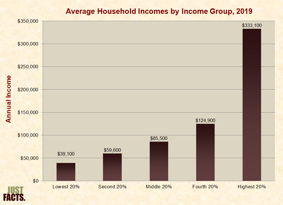
* According to data from the Congressional Budget Office, U.S. households had an average income of $125,500 in 2019 prior to the Covid-19 pandemic.[46] This includes income sources like wages, salaries, capital gains, rental income, and untaxed government and employer-provided benefits like food stamps and health insurance. This varied by income group as follows:
* According to data from the Congressional Budget Office, U.S. households had an average income of $133,000 in 2020 amid Covid-19 government lockdowns and intensified social spending:[49] [50] [51]
* From 1979 to 2019 (prior to the Covid-19 pandemic,[54]) the inflation-adjusted average income of U.S. households increased by $54,300 or 76%. This varied by income group as follows:
|
Inflation-Adjusted Household Income |
||||
|
Income Group |
1979 |
2019 |
Increase From 1979 to 2019 |
|
|
Dollars |
Percent |
|||
|
Lowest 20% |
$21,500 |
$39,100 |
$17,600 |
82% |
|
Second 20% |
$40,200 |
$59,600 |
$19,400 |
48% |
|
Middle 20% |
$60,600 |
$85,500 |
$24,900 |
41% |
|
Fourth 20% |
$82,000 |
$124,900 |
$42,900 |
52% |
|
Highest 20% |
$155,100 |
$333,100 |
$178,000 |
115% |
|
Top 1% |
$595,300 |
$1,998,700 |
$1,403,400 |
236% |
|
All Groups |
$71,200 |
$125,500 |
$54,300 |
76% |
* From 1979 to 2020 (amid Covid-19 government lockdowns and intensified social spending,[57] [58] [59]) the inflation-adjusted average income of U.S. households increased by $61,000 or 85%. This varied by income group as follows:
|
Inflation-Adjusted Household Income |
||||
|
Income Group |
1979 |
2020 |
Increase From 1979 to 2020 |
|
|
Dollars |
Percent |
|||
|
Lowest 20% |
$21,800 |
$42,200 |
$20,400 |
94% |
|
Second 20% |
$40,700 |
$63,600 |
$22,900 |
56% |
|
Middle 20% |
$61,300 |
$90,500 |
$29,200 |
48% |
|
Fourth 20% |
$82,900 |
$131,800 |
$48,900 |
59% |
|
Highest 20% |
$156,800 |
$360,900 |
$204,100 |
130% |
|
Top 1% |
$602,000 |
$2,291,800 |
$1,689,800 |
281% |
|
All Groups |
$72,000 |
$133,000 |
$61,000 |
85% |
* After federal taxes, the inflation-adjusted average income of U.S. middle-income households rose from $49,700 in 1979 to $84,300 in 2020, or by $34,600 or 70%:
[62] [63] [64] [65] [66] [67] [68]
* After federal taxes, the inflation-adjusted average income of U.S. households rose by $46,800 or 84% during 1979 to 2019 (prior to the Covid-19 pandemic.[69]) This varied by income group as follows:
|
Inflation-Adjusted Household Income After Federal Taxes |
||||
|
Income Group |
1979 |
2019 |
Increase From 1979 to 2019 |
|
|
Dollars |
Percent |
|||
|
Lowest 20% |
$20,100 |
$38,900 |
$18,800 |
94% |
|
Second 20% |
$34,300 |
$54,900 |
$20,600 |
60% |
|
Middle 20% |
$49,100 |
$74,800 |
$25,700 |
52% |
|
Fourth 20% |
$64,300 |
$104,400 |
$40,100 |
62% |
|
Highest 20% |
$113,100 |
$252,100 |
$139,000 |
123% |
|
Top 1% |
$386,700 |
$1,398,500 |
$1,011,800 |
262% |
|
All Groups |
$55,600 |
$102,400 |
$46,800 |
84% |
* After federal taxes, the inflation-adjusted average income of U.S. households rose by $56,500 or 101% during 1979 to 2020 (amid Covid-19 government lockdowns and intensified social spending.[73] [74] [75]) This varied by income group as follows:
|
Inflation-Adjusted Household Income After Federal Taxes |
||||
|
Income Group |
1979 |
2020 |
Increase From 1979–2020 |
|
|
Dollars |
Percent |
|||
|
Lowest 20% |
$20,300 |
$45,800 |
$25,500 |
126% |
|
Second 20% |
$34,700 |
$63,200 |
$28,500 |
82% |
|
Middle 20% |
$49,700 |
$84,300 |
$34,600 |
70% |
|
Fourth 20% |
$65,000 |
$115,100 |
$50,100 |
77% |
|
Highest 20% |
$114,300 |
$275,700 |
$161,400 |
141% |
|
Top 1% |
$391,000 |
$1,605,400 |
$1,214,400 |
311% |
|
All Groups |
$56,200 |
$112,700 |
$56,500 |
101% |
* The two main categories of income are:
* Private charities provide other sources of non-cash income to low-income people. These include but are not limited to food, clothing, housing, and healthcare.[81] [82] [83] [84]
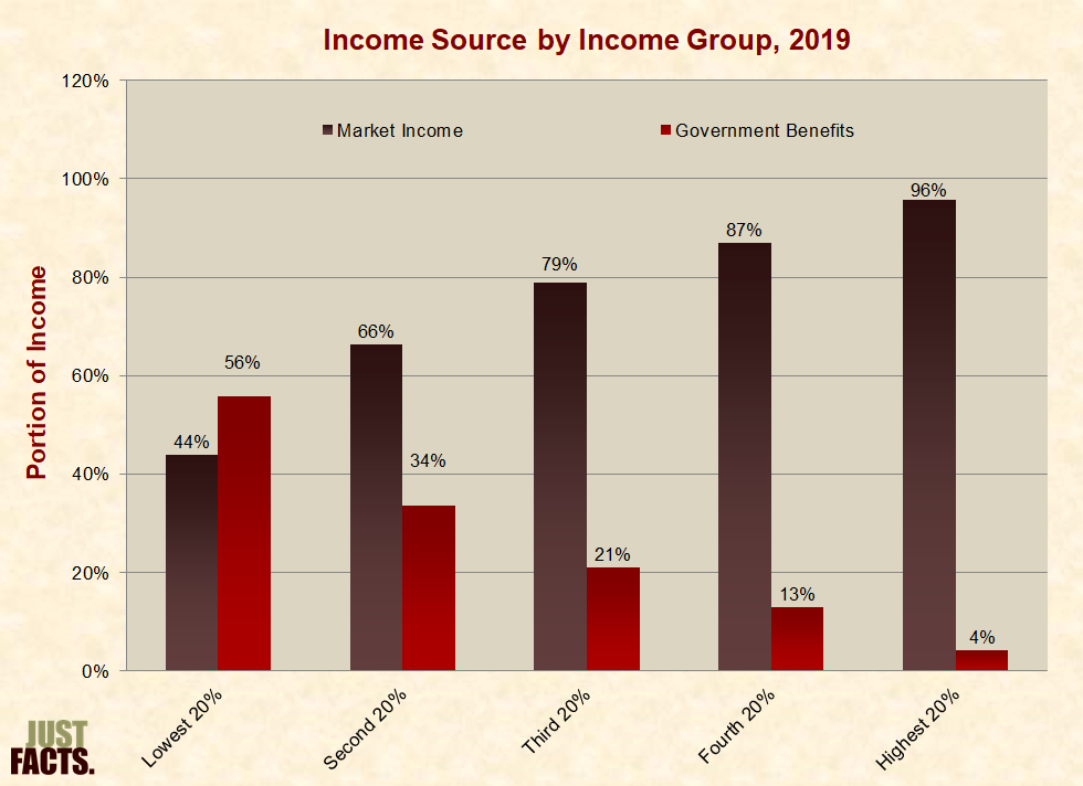
* According to data from the Congressional Budget Office, U.S. households obtained about 86% of their income from the market and 14% from the government in 2019 prior to the Covid-19 pandemic.[85] This varied by income group on average as follows:
* According to data from the Congressional Budget Office, U.S. households obtained about 82% of their income from the market and 18% from the government in 2020 amid Covid-19 government lockdowns and intensified social spending.[88] [89] [90] This varied by income group on average as follows:
* From 1979 to 2019 (prior to the Covid-19 pandemic,[93]) government benefits rose from 9% of total household income to 14%, or by 60%. This varied by income group as follows:
|
Average Portion of Household Income From Government Benefits |
||||
|
Income Group |
1979 |
2019 |
Change |
|
|
Percentage Points |
Percent |
|||
|
Lowest 20% |
51% |
56% |
5 |
9% |
|
Second 20% |
19% |
34% |
15 |
77% |
|
Middle 20% |
8% |
21% |
13 |
155% |
|
Fourth 20% |
5% |
13% |
8 |
168% |
|
Highest 20% |
2% |
4% |
2 |
74% |
|
All Groups |
9% |
14% |
5 |
60% |
* From 1979 to 2020 (amid Covid-19 government lockdowns and intensified social spending,[96] [97] [98]) government benefits rose from 9% of total household income to 18%, or by 100%. This varied by income group as follows:
|
Average Portion of Household Income From Government Benefits |
||||
|
Income Group |
1979 |
2020 |
Change |
|
|
Percentage Points |
Percent |
|||
|
Lowest 20% |
51% |
64% |
13 |
25% |
|
Second 20% |
19% |
42% |
23 |
120% |
|
Middle 20% |
8% |
27% |
19 |
227% |
|
Fourth 20% |
5% |
16% |
12 |
241% |
|
Highest 20% |
2% |
5% |
2 |
99% |
|
All Groups |
9% |
18% |
9 |
100% |
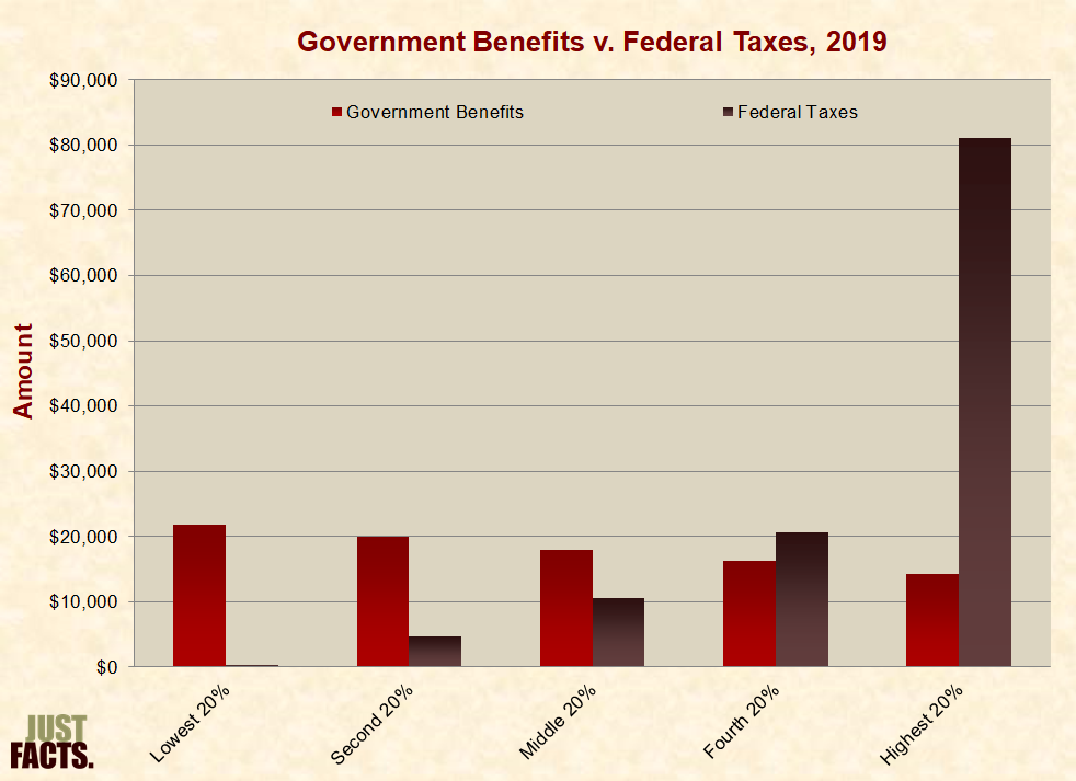
* In 2019, prior to the Covid-19 pandemic,[101] roughly 60% of U.S. households received more in federal, state, and local government benefits than they paid in federal taxes:
* In 2020, amid Covid-19 government lockdowns and intensified social spending,[105] [106] [107] roughly 80% of U.S. households received more in federal, state, and local government benefits than they paid in federal taxes:
* In 1979, only the lowest-income 20% of U.S. households and the second lowest 20% received more in federal, state, and local government benefits than they paid in federal taxes. Since then, the following households have also moved into this territory:
* Government benefits can suppress market income by:
* According to data from the Congressional Budget Office, cash wages and salaries accounted for 62% of market income to U.S. households in 2020. Capital and business income provided 29%, and employer-paid benefits made up the remaining 8%. This varied by income group as follows:
* According to data from the Congressional Budget Office, benefits paid by employers accounted for 11% of middle-income worker compensation in 1979. By 2020, this figure had risen to 15%. This varied by income group as follows:
|
Portion of Worker Compensation in Benefits |
||
|
Income Group |
1979 |
2020 |
|
Lowest 20% |
11% |
14% |
|
Second 20% |
12% |
15% |
|
Middle 20% |
11% |
15% |
|
Fourth 20% |
10% |
14% |
|
Highest 20% |
9% |
10% |
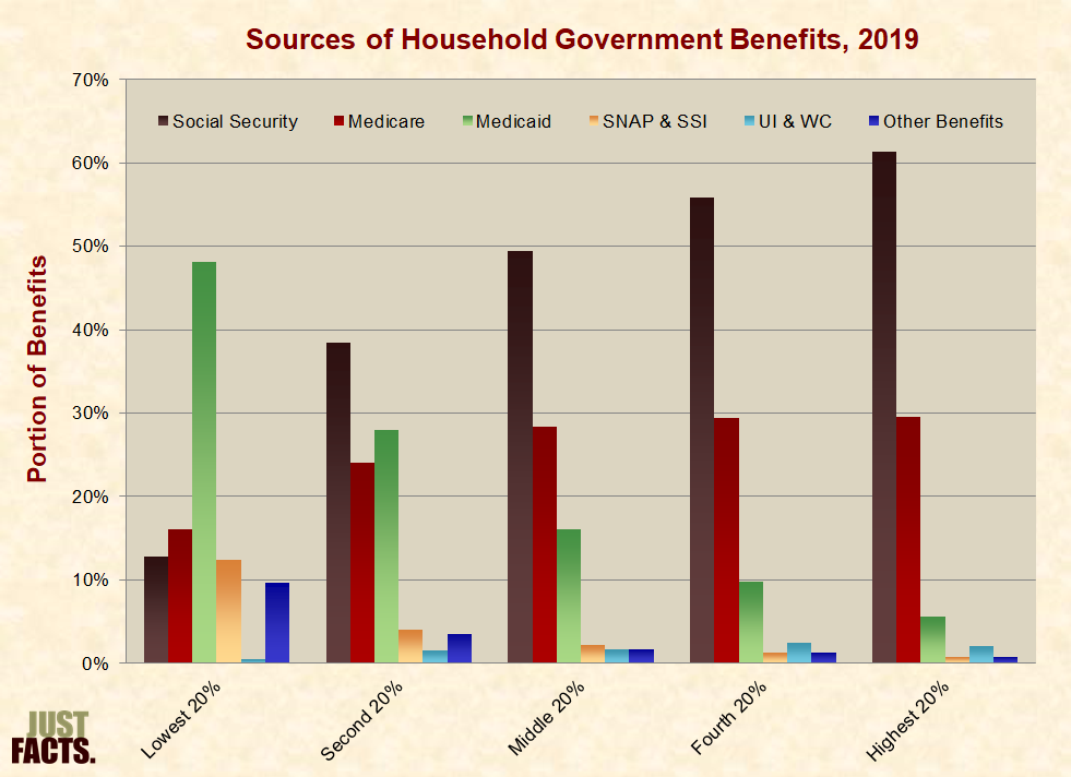
* The two largest sources of household government income are Social Security and Medicare, both of which benefit elderly and disabled people.[132] [133] [134]
* In June of 2021, 65.0 million people—20% of the U.S. population—received Social Security benefits.[135]
* In 2021, 63.8 million people—19% of the U.S. population—received Medicare benefits.[136]
* According to data from the Congressional Budget Office, in 2019 prior to the Covid-19 pandemic:[137]
* According to data from the Congressional Budget Office, in 2020 amid Covid-19 government lockdowns and intensified social spending:[142] [143] [144]
* “Personal consumption” is a comprehensive measure of the goods and services consumed by households. In the United States, consumption is recorded by the federal government’s Bureau of Economic Analysis and includes all material resources:
* Per the World Bank:[152]
* Per a 2003 paper in the Journal of Human Resources:
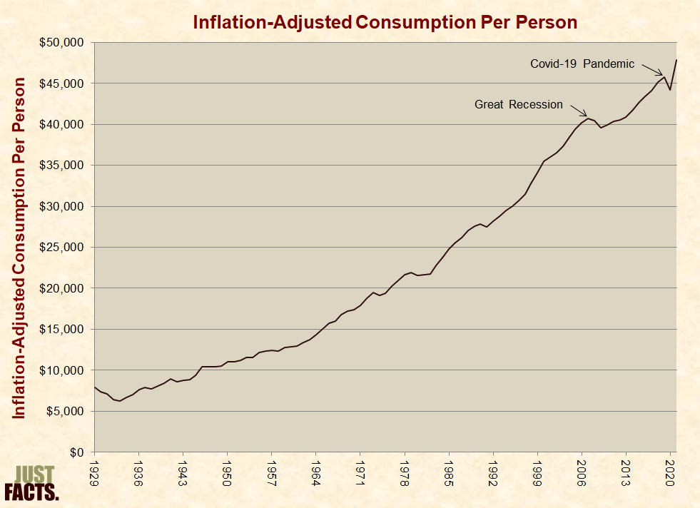
* In the United States from 1929 to 2021, the average inflation-adjusted consumption per person rose by 5.1 times:
* Most U.S. households—especially lower-income ones—consume more goods and services than revealed by common measures of income.[160] [161] [162] This is because widely used income measures, like the Census Bureau’s “money income”:
* With regard to the exclusion of noncash benefits from common income measures:
* With regard to the underreporting of income on government household surveys:
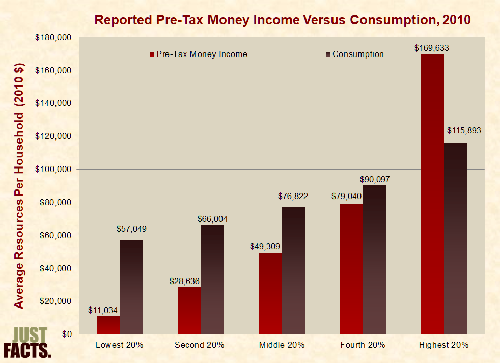
* The U.S. Bureau of Economic Analysis normally reports consumption for the entire nation and doesn’t break down the data to show how people at different levels fare. However, it published a report in 2012 that does that for 2010.[204]
* In 2010, the poorest 20% of U.S. households consumed on average of $57,049 of goods and services per household, while they reported an average of $11,034 in pre-tax money income. For other households, the amounts varied as follows:
* The U.S. Bureau of Labor Statistics collects data on a subset of consumption called “consumer expenditures.” This includes all direct purchases by households, including those made with the proceeds of government benefits like cash welfare and food stamps. However, it excludes goods and services received but not directly purchased by households, such as Medicaid, Medicare, housing subsidies, school lunches, and employer-provided health insurance.[207] [208] [209] [210] [211] [212]
* The Department of Labor collects data on consumer expenditures via household surveys.[213] Per the U.S. Bureau of Economic Analysis, such surveys “have issues with recalling income and expenditures and are subject to deliberate underreporting of certain items.”[214] [215]
* The average consumer expenditures of the poorest 10% of U.S. households are 4.4 times their reported, before-tax, money income. The ratios of spending to income for other groups varied as follows:
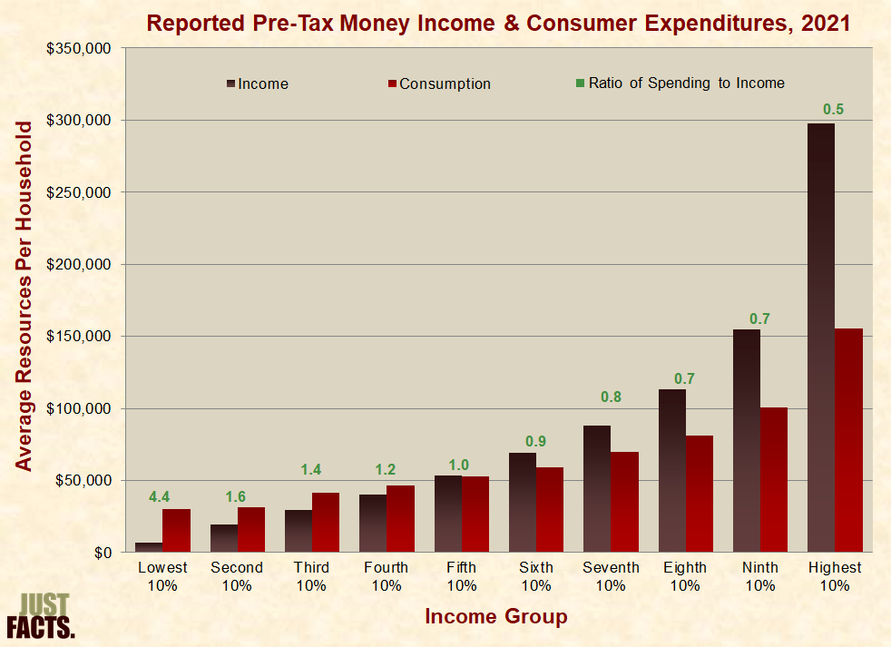
* The Department of Labor explains that consumers can temporarily spend more than their income by borrowing or “drawing down savings and investments.”[218] Thus, some people in the lowest income group “have expenditures that are more typical of upper-income consumers.”[219]
* From 1984 to 2021, the average inflation-adjusted consumer expenditures per household varied as follows:
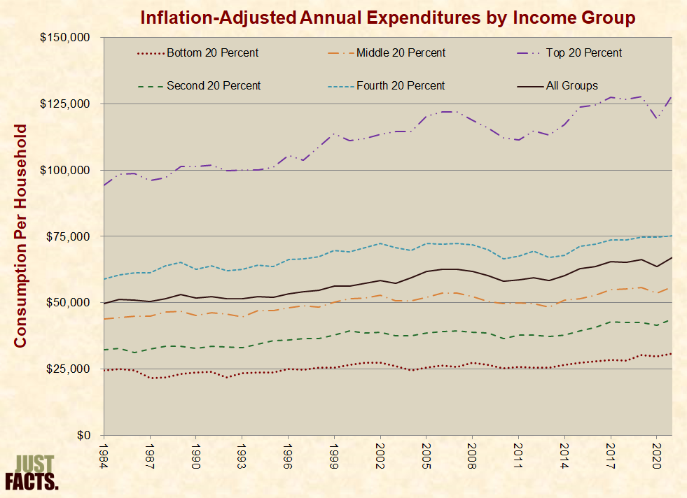
* From 1984 to 2021, the average inflation-adjusted consumer expenditures of the bottom 20% of households increased by $6,306. This gain closed the 1984 gap between the bottom 20% and the next income group by 81%. The gap closures between the other groups varied as follows:
|
Inflation-Adjusted Consumer Expenditures |
|||
|
Income Group |
Year |
Portion of 1989 Gap Closed |
|
|
1984 |
2021 |
||
|
Bottom 20 Percent |
$24,563 |
$30,869 |
81% |
|
Second 20 Percent |
$32,326 |
$43,918 |
100% |
|
Middle 20 Percent |
$43,897 |
$55,914 |
80% |
|
Fourth 20 Percent |
$58,934 |
$75,284 |
46% |
|
Top 20 Percent |
$94,304 |
$128,213 |
– |
* Per the U.S. Bureau of Labor Statistics, “consumption patterns indicate the priorities that families place on the satisfaction of the following needs”:
* In 2021, households spent 21% of their consumer expenditures on shelter:
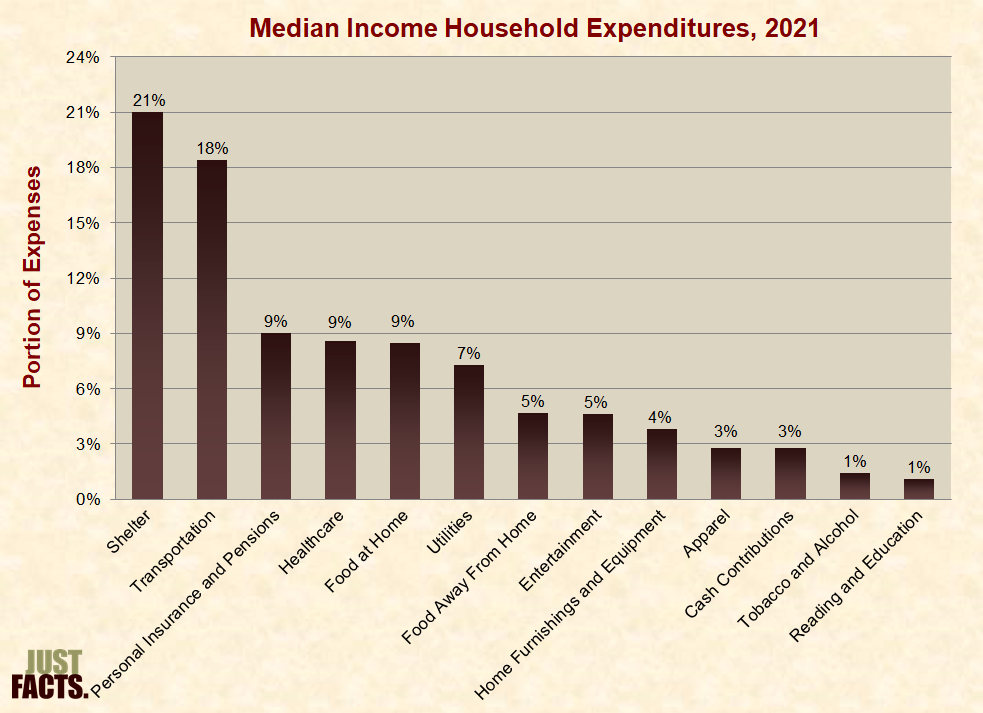
* In 1901, U.S. households spent 43% of their income on food. By 2021, spending on food had decreased to 12% of income. The spending levels for other expenses varied as follows:
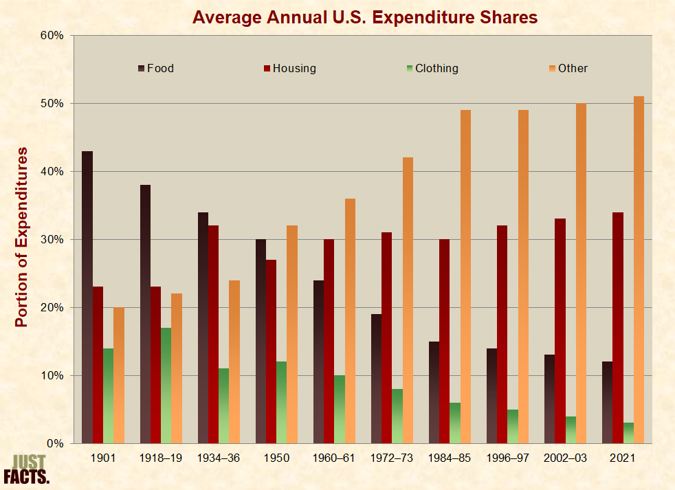
* Per a 2006 report by the Bureau of Labor Statistics:
* In 2020, 88% of U.S. homes had air conditioning. The average usage or possession rates for air conditioning and other appliances varied by income group as follows:
|
Average Usage or Possession Rates by Income Group |
||||
|
Income Group |
Appliance |
|||
|
Air Conditioning |
Dishwasher |
Clothes Washer |
Clothes Dryer |
|
|
Less than $20,000 |
80% |
38% |
61% |
58% |
|
$20,000 to $40,000 |
87% |
61% |
80% |
78% |
|
$40,000 to $60,000 |
88% |
72% |
85% |
84% |
|
$60,000 to $100,000 |
90% |
83% |
90% |
90% |
|
$100,000 to $150,000 |
93% |
90% |
93% |
93% |
|
$150,000 or More |
93% |
95% |
95% |
94% |
|
All Homes |
88% |
73% |
84% |
83% |
* As of 2020, 93% of U.S. homes had internet access. The average usage and possession rates for different types of electronic devices and services varied by income as follows:
|
Average Usage or Possession Rates by Income Group |
||||
|
Income Group |
Electronic Device or Service |
|||
|
Primary TV 40” or Larger |
Cable & Digital Video Recorder |
Internet Access |
Smartphone |
|
|
Less than $20,000 |
53% |
20% |
76% |
72% |
|
$20,000 to $40,000 |
65% |
29% |
89% |
80% |
|
$40,000 to $60,000 |
71% |
33% |
95% |
89% |
|
$60,000 to $100,000 |
77% |
37% |
98% |
94% |
|
$100,000 to $150,000 |
80% |
40% |
99% |
96% |
|
$150,000 or More |
85% |
47% |
100% |
98% |
|
All Homes |
72% |
34% |
93% |
88% |
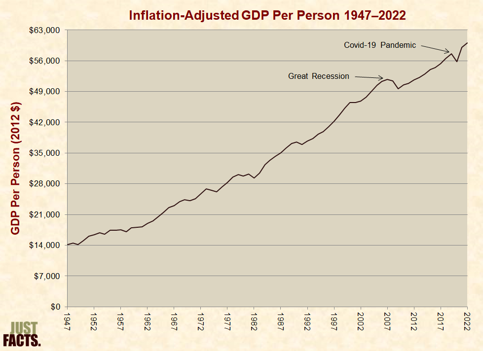
* Gross domestic product (GDP) is the standard measure of nations’ economic output. It is equal to the value of all goods and services that a country produces in a year minus the resources used to produce them. GDP is defined by the equation: Hours worked × Labor productivity.[233] [234]
* GDP divided by the population is often used to measure a country’s standard of living. Per the textbook Macroeconomics for Today:
* In the U.S. from 1947 to 2022, the average inflation-adjusted GDP per person rose by 4.2 times:[236]
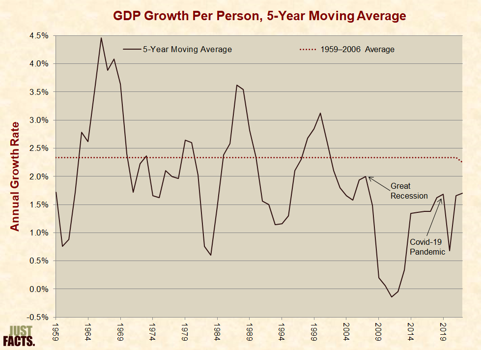
* Inflation-adjusted GDP growth per person in the U.S. has varied as follows since 1959:
* In 2012, the Journal of Economic Perspectives published a paper about the economic consequences of government debt. Using 2,000+ data points on national debt and economic growth in 20 advanced economies (such as the United States, France, and Japan) from 1800 to 2009, the authors found that countries with national debts above 90% of GDP averaged 34% less real annual economic growth than when their debts were below 90% of GDP.[245]
* At the close of 2022, the debt/GDP level in the U.S. was 123%.[246]
* In 2013, the Political Economy Research Institute at the University of Massachusetts, Amherst, published a paper about the economic consequences of government debt. Using data on national debt and economic growth in 20 advanced economies from 1946 to 2009, the authors found that countries with national debts over 90% of GDP averaged:
* The authors of the above-cited papers have engaged in a heated dispute about the results of their respective papers and the effects of government debt on economic growth. Facts about these issues can be found in Just Facts’ article, “Do Large National Debts Harm Economies?“
* “Personal consumption” is a comprehensive measure of the goods and services consumed by households. It includes all material resources:
* Per the World Bank:[250]
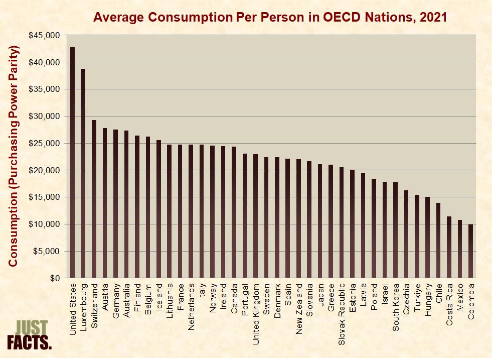
* The Organization for Economic Cooperation and Development (OECD) is an international association that is mainly comprised of wealthy, developed nations.[253] [254] In 2021, the United States had the highest average consumption per person of all 38 nations in the OECD:
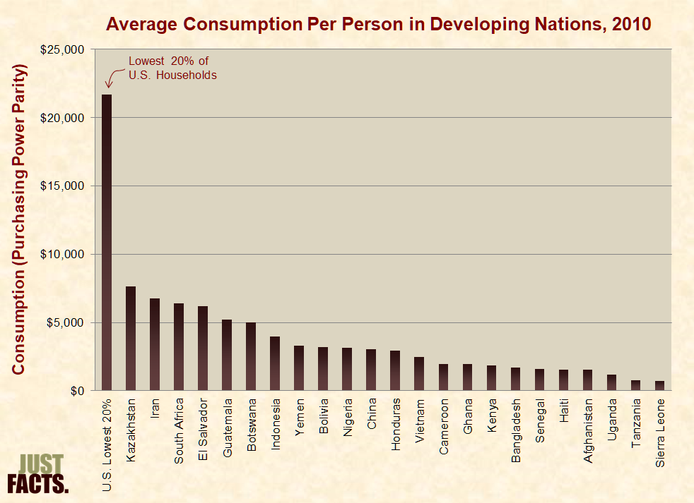
* The federal government’s Bureau of Economic Analysis—which is the source of consumption data for the United States—normally reports consumption for the entire nation and doesn’t break down the data to show how people at different levels fare. However, it published a report that does that for 2010.[258] Combined with World Bank data for the same year, these datasets show that:
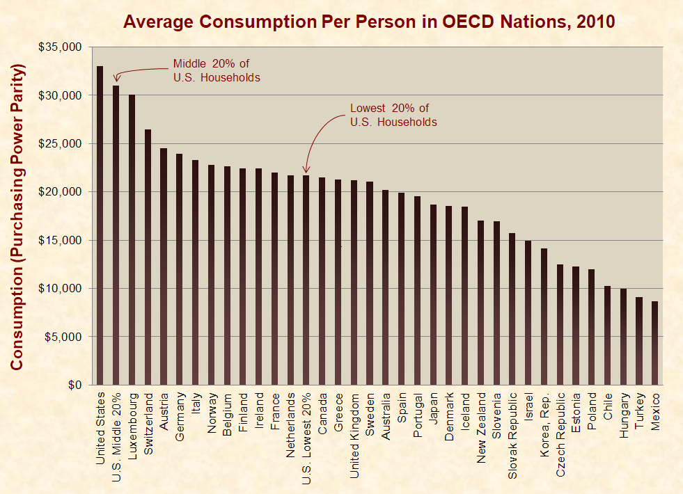
* In 2010, the poorest 20% of Americans consumed three to 30 times more goods and services on average than the national averages for all people in an array of developing nations:
* For an article and video by Just Facts about how the New York Times misled the public about poverty in the U.S. compared to other nations, click here.
* Gross domestic product (GDP) is the standard measure of nations’ economic output. It is equal to the value of all goods and services that a country produces in a year minus the resources used to produce them.[264] [265]
* Per the U.S. Bureau of Labor Statistics:
* Per the textbook Macroeconomics for Today:
* In 2021, the worldwide average GDP per person was $16,997. This varied from a high of $62,403 in North America to a low of $3,717 in Sub-Saharan Africa:

* In 2021, the U.S. ranked 5th among 41 developed nations in average GDP per person. Other developed nations ranked as follows:

* Per the Organization for Economic Cooperation and Development:
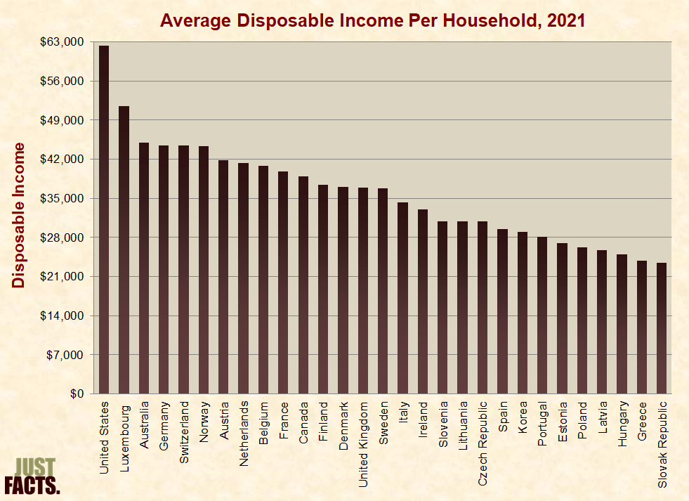
* Household disposable income equals:
* In 2021, the United States ranked first among 29 developed nations in average disposable income per household:
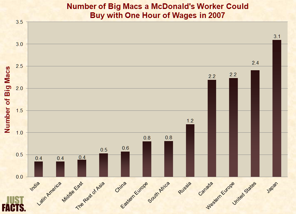
* Real wages are a measure of the goods that workers can buy with the money they earn from one hour of work.[276]
* In 2012, the American Economic Review published a paper by Princeton University economist Orley Ashenfelter that compared the real wages of McDonald’s workers in over 60 countries. He did this by determining how many Big Macs they could buy with their income from an hour of work. The advantage of using this measure is that:
* The study found that McDonald’s workers in the United States had the second-highest real wages of McDonald’s workers in all economic regions:
* Labor productivity is the amount of goods and services that workers produce in an hour.[279] [280] [281] [282]
* Per Federal Reserve Chair Janet Yellen (and various other economists with wide-ranging political views):
* Per the Congressional Budget Office, “a small change in the growth of productivity” over an extended period can do more harm than recessions, because low labor productivity reduces economic “output by an ever-increasing amount.”[290]
* As an example of labor productivity growth, U.S. businesses increased their inflation-adjusted output by 42% from 1998 to 2013 without any increase in work hours.[291]
* Labor productivity growth is driven by three primary factors:
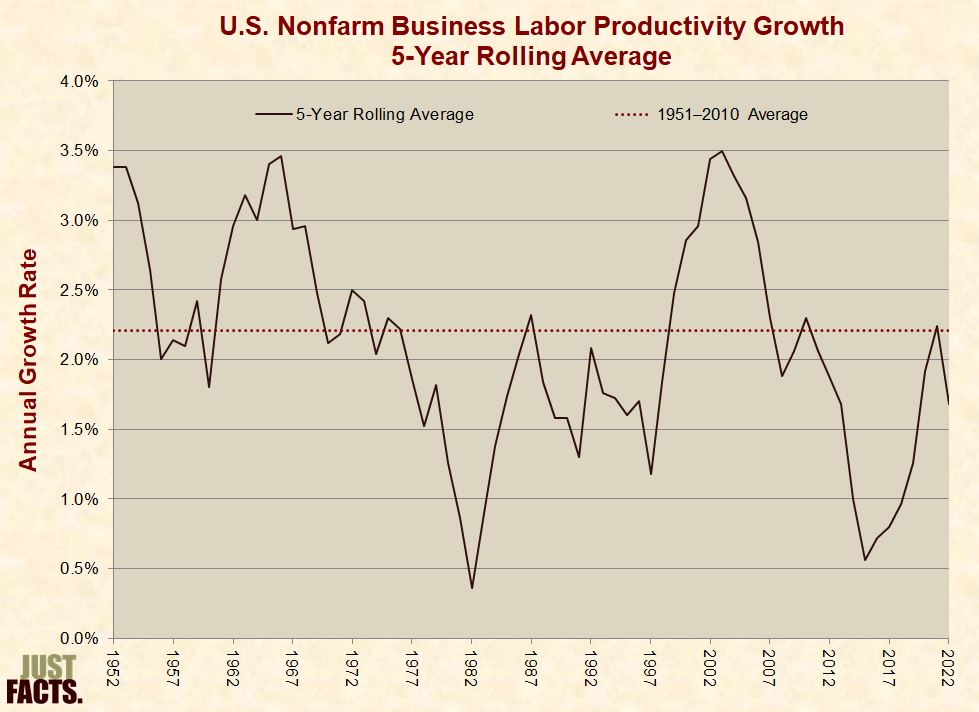
* Because productivity growth often fluctuates over the short term, it is sometimes measured in five-year moving averages.[295] [296]
* The U.S. Bureau of Labor Statistics considers the nonfarm business sector to be the best single indicator of labor productivity for the U.S. economy. This is because it excludes sectors that are volatile or don’t produce concretely measurable output.[297] [298] [299]
* Nonfarm labor productivity growth in the U.S. has varied as follows since 1952:
* If the labor productivity slowdown that took place from 2005 to 2015 had not occurred, the U.S. economy in 2015 would have been about $3 trillion larger. This amounts to an average of $24,100 for every household in the United States.[301]
* Productivity growth can be suppressed by a variety of factors, such as:
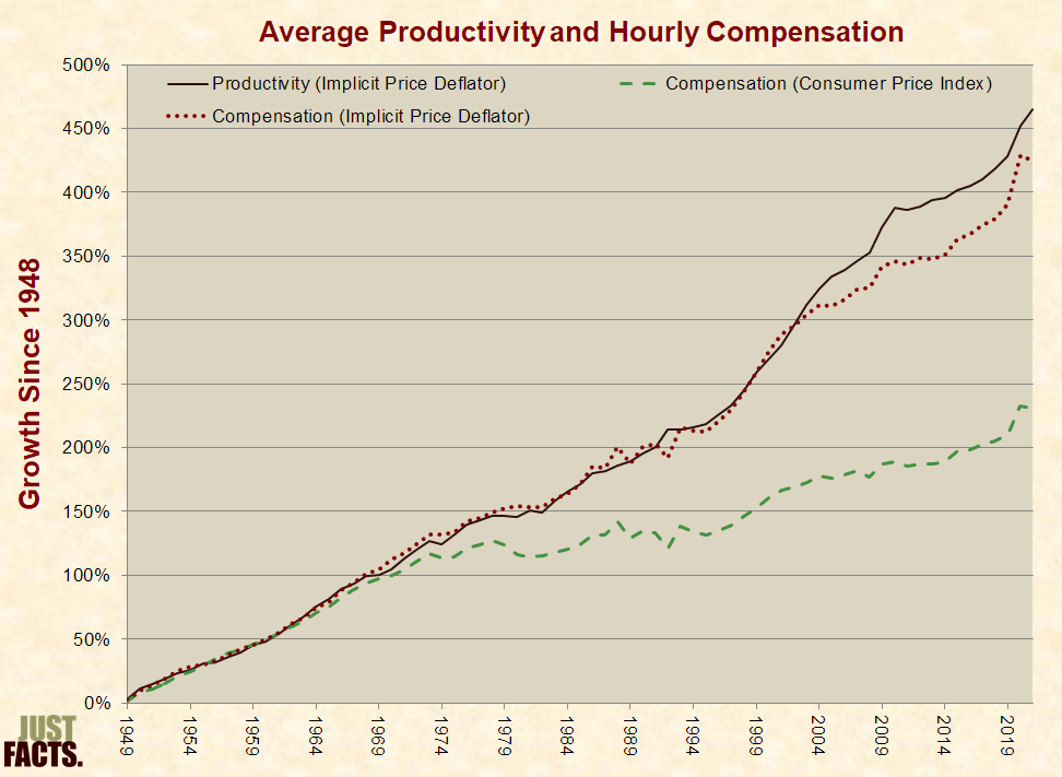
* Some politicians, commentators, and policy analysts have claimed that worker compensation has risen more slowly than worker productivity for decades, such as:
* Per Ph.D. economist Martin Feldstein, professor of economics at Harvard University and President Emeritus of the National Bureau of Economic Research:[321]
* Another reason behind claims that worker compensation has not kept pace with productivity growth is that some studies compare the compensation of one group of workers to the productivity of another group of workers.[323] [324]
* An objective comparison of labor productivity and compensation requires that:
* The U.S. government typically adjusts:
* When adjusted for inflation using:
* Beyond economic trends in earnings, profits, and government benefits—household incomes are affected by social factors like divorce, cohabitation, single parenting, and dual-income families.[341]
* According to data from the Congressional Budget Office, the inflation-adjusted average income of U.S. households rose by 76% between 1979 and 2019 (prior to the Covid-19 pandemic.)[342] For various income groups, it grew as follows:

* According to data from the Congressional Budget Office, the inflation-adjusted average income of U.S. households rose by 85% between 1979 and 2020 (amid Covid-19 government lockdowns and intensified social spending.)[345] [346] [347] For various income groups, it grew as follows:
* From 1979 to 2019 (prior to the Covid-19 pandemic),[350] the inflation-adjusted average income of U.S. households after federal taxes rose by about $46,800 or 84%. For various income groups, it grew as follows:
|
Inflation-Adjusted Household Income After Federal Taxes |
||||
|
Income Group |
1979 |
2019 |
Increase From 1979 to 2019 |
|
|
Dollars |
Percent |
|||
|
Lowest 20% |
$20,100 |
$38,900 |
$18,800 |
94% |
|
Second 20% |
$34,300 |
$54,900 |
$20,600 |
60% |
|
Middle 20% |
$49,100 |
$74,800 |
$25,700 |
52% |
|
Fourth 20% |
$64,300 |
$104,400 |
$40,100 |
62% |
|
Highest 20% |
$113,100 |
$252,100 |
$139,000 |
123% |
|
Top 1% |
$386,700 |
$1,398,500 |
$1,011,800 |
262% |
|
All Groups |
$55,600 |
$102,400 |
$46,800 |
84% |
* From 1979 to 2020 (amid Covid-19 government lockdowns and intensified social spending),[354] [355] [356] the inflation-adjusted average income of U.S. households after federal taxes rose by about $56,500 or 101%. For various income groups, it grew as follows:
|
Inflation-Adjusted Household Income After Federal Taxes |
||||
|
Income Group |
1979 |
2020 |
Increase From 1979 to 2020 |
|
|
Dollars |
Percent |
|||
|
Lowest 20% |
$20,300 |
$45,800 |
$25,500 |
126% |
|
Second 20% |
$34,700 |
$63,200 |
$28,500 |
82% |
|
Middle 20% |
$49,700 |
$84,300 |
$34,600 |
70% |
|
Fourth 20% |
$65,000 |
$115,100 |
$50,100 |
77% |
|
Highest 20% |
$114,300 |
$275,700 |
$161,400 |
141% |
|
Top 1% |
$391,000 |
$1,605,400 |
$1,214,400 |
311% |
|
All Groups |
$56,200 |
$112,700 |
$56,500 |
101% |
* From 1979 to 2019 (prior to the Covid-19 pandemic),[360] U.S. middle-income households’ share of total income after federal taxes decreased by about 1.9 percentage points, or by 12%. The share of income for other groups changed as follows:
|
Share of Total Income After Federal Taxes |
||||
|
Income Group |
1979 |
2019 |
Change |
|
|
Percentage Points |
Percent |
|||
|
Lowest 20% |
7.8% |
7.7% |
–0.1 |
–1% |
|
Second 20% |
12.3% |
10.7% |
–1.6 |
–13% |
|
Middle 20% |
16.4% |
14.5% |
–1.9 |
–12% |
|
Fourth 20% |
22.1% |
20.2% |
–1.9 |
–9% |
|
Highest 20% |
41.8% |
48.5% |
6.7 |
16% |
|
Top 1% |
7.4% |
13.0% |
5.6 |
76% |
* From 1979 to 2020 (amid Covid-19 government lockdowns and intensified social spending),[364] [365] [366] U.S. middle-income households’ share of total income after federal taxes decreased by about 1.4 percentage points, or by 9%. The share of income for other groups changed as follows:
|
Share of Total Income After Federal Taxes |
||||
|
Income Group |
1979 |
2020 |
Change |
|
|
Percentage Points |
Percent |
|||
|
Lowest 20% |
7.8% |
8.2% |
0.4 |
5% |
|
Second 20% |
12.3% |
11.4% |
–0.9 |
–7% |
|
Middle 20% |
16.4% |
15.0% |
–1.4 |
–9% |
|
Fourth 20% |
22.1% |
20.0% |
–2.1 |
–10% |
|
Highest 20% |
41.8% |
46.8% |
5.0 |
12% |
|
Top 1% |
7.4% |
13.2% |
5.8 |
78% |
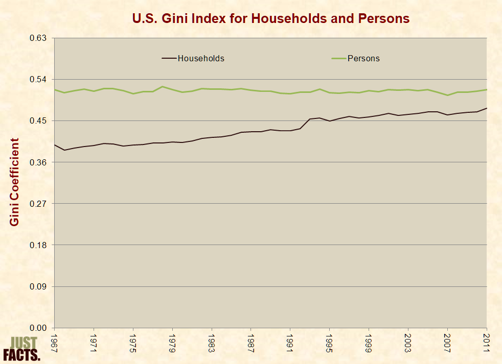
* The Gini index is the most common measure of income inequality.[370] [371] [372]
* Various reporters at major media outlets have cited the Gini index for household income to claim that:
* A 2014 study published by the Social Science Research Network found that:
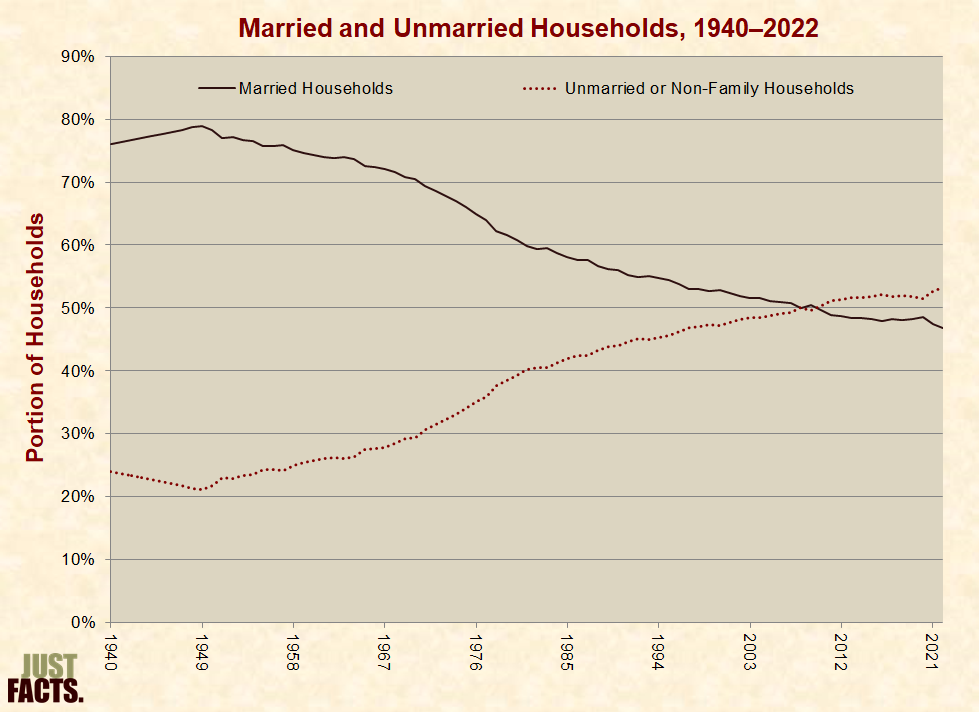
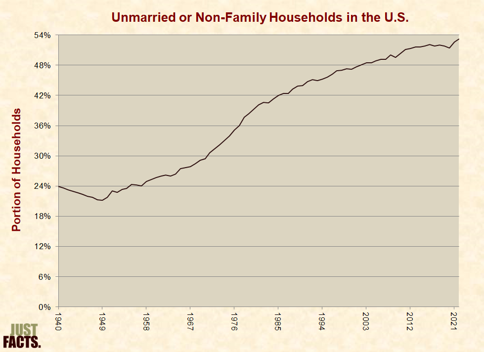
* From 1940 to 2022, the number of households in the U.S. increased by 275%, while the U.S. population increased by 152%.[377] [378] During this same period, the portion of unmarried or non-family households rose from 24% to 53%:
* From 1967 to 2011:
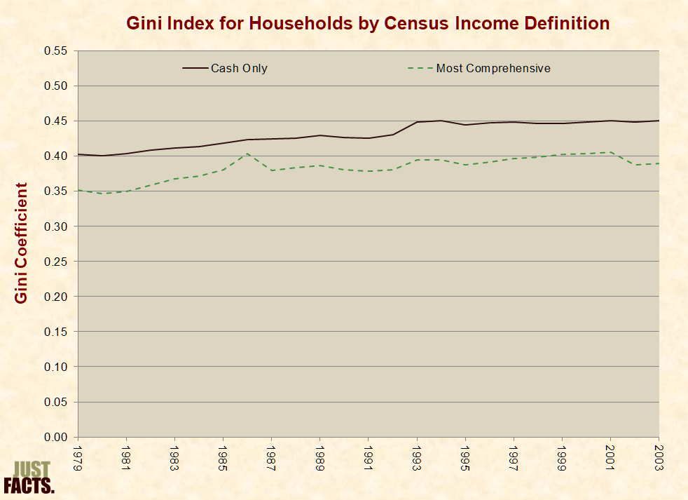
* The standard Gini index published by the Census Bureau does not include all income and taxes.[381] From 1979 to 2003, the Census Bureau published Gini index data based on more comprehensive measures of income.[382] [383] Over this period, the standard Gini index averaged 12% higher than the Gini index based on the most comprehensive Census income measure:
* All Gini indexes based on Census Bureau data are derived from surveys, and households often underreport their cash and noncash income on such surveys.[385] [386]
* Per a 2015 paper in the Journal of Economic Perspectives entitled “Household Surveys in Crisis”:
* An analysis of Federal Reserve data published by Rice University’s Baker Institute for Public Policy found that income inequality fell between 2016 and 2019. The decline was the largest since 1992.[390]
* During his acceptance speech at the 2016 Republican National Convention, Donald Trump made the following claim, and New York Times and NPR reported that it was “true”:
* This claim is based on data from the U.S. Census Bureau,[394] which:
* More comprehensive data from the Congressional Budget Office shows that the inflation-adjusted average household income of the middle 20% of U.S. households rose from $72,100 in 2000 to $81,500 in 2016, or by $9,2400 or 13%. After federal taxes, their income climbed by $10,600 or 18%.[401] [402] [403]
* To adjust income data for inflation, the Congressional Budget Office uses the Personal Consumption Expenditure price index.[404] [405] If it were adjusted for inflation using the Consumer Price Index, this same data would show that from 2000 to 2016, average middle-class household income rose by $6,361 or 8%, and average middle-class household income after federal taxes rose by $8,161 or 13%.[406] [407] [408]
* In 2015, U.S. Senator Elizabeth Warren of Massachusetts made the following claim based on data from tax returns, and PolitiFact said it was “mostly true”:
* More comprehensive data from the Congressional Budget Office shows that the inflation-adjusted average income of households in the bottom 90% rose from $55,527 in 1980 to $83,591 in 2015, or by 51%. After federal taxes, their income climbed from $44,922 in 1980 to $71,527 in 2015, or by $26,606 or 59%.[411] [412] [413]
* In 2013, the Pew Research Center claimed that:
* More comprehensive data from the Congressional Budget Office shows that in 2012, the top 1% received 18% of all pretax income, and the bottom 90% received 62%. The distribution of pretax income since 1979 has varied as follows:

* After federal taxes, the top 1% received 15% of all household income in 2012, and the bottom 90% received 66%. The distribution of income after federal taxes since 1979 has varied as follows:
* The claims above from PolitiFact (2015), and Pew Research (2013), are based on the work of Ph.D. economists Thomas Piketty and Emmanuel Saez.[420] [421] Paul Krugman of the New York Times has called their work on income inequality a “landmark piece of research that has had a major impact.”[422]
* Piketty and Saez have published articles and academic papers that overstate income inequality by:
* The income share of the top 10%—as estimated by Piketty and Saez in 2017, Piketty and Saez in 2022, and the Congressional Budget Office in 2022—have varied as follows:
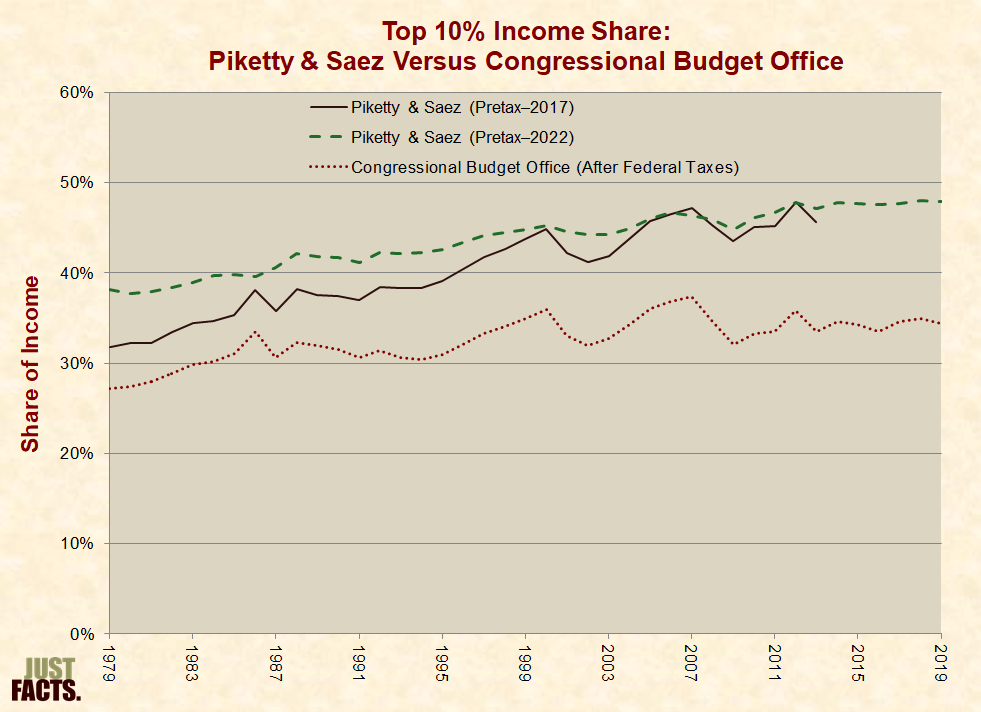 |
NOTE: This chart does not account for the rise in number of households, which would reduce the income share growth of the top 10% over time.[443] |
* According to Piketty and Saez, “the average federal tax burden on top 1% families has decreased from 44.4% in 1980 to 30.4% in 2004,” or by 14 percentage points.[444]
* More comprehensive tax and income data from the Congressional Budget Office shows that the average federal tax burden on the top 1% of households decreased from about 33% in 1980 to 30% in 2004, or by 3 percentage points.[445] [446] [447]
* According to Piketty and Saez, from 1980 to 2004, the total decrease in federal taxes paid by the top 1% was greater than the total increase in government benefits received by the bottom 99%.[448]
* More comprehensive inflation-adjusted data from the Congressional Budget Office shows that from 1980 to 2004:
* In 1997, the Journal of Economic Behavior & Organization published a survey of 247 faculty, students, and staff at the Harvard School of Public Health. This survey:
* In 2015, U.S. residents of varying income, race, education, and marital status described their overall economic well-being as follows:
|
Self-Perception of Overall Economic Well-Being |
||||
|
Characteristic |
Finding It Difficult to Get By |
Just Getting By |
Doing Okay |
Living Comfortably |
|
Family Income |
||||
|
Less than $40,000 |
18% |
32% |
39% |
12% |
|
$40,000–$100,000 |
4% |
19% |
47% |
29% |
|
Greater than $100,000 |
2% |
8% |
37% |
54% |
|
Race/Ethnicity |
||||
|
White, non-Hispanic |
9% |
20% |
41% |
30% |
|
Black, non-Hispanic |
10% |
28% |
41% |
20% |
|
Hispanic |
12% |
25% |
43% |
21% |
|
Education |
||||
|
High school degree or less |
13% |
26% |
41% |
20% |
|
Some college or associate degree |
9% |
25% |
42% |
24% |
|
Bachelor’s degree or more |
6% |
14% |
40% |
41% |
|
Marital and Parental Status |
||||
|
Unmarried, no children under 18 |
12% |
25% |
42% |
21% |
|
Married, no children under 18 |
6% |
15% |
43% |
37% |
|
Unmarried, children under 18 |
19% |
34% |
34% |
13% |
|
Married, children under 18 |
7% |
22% |
40% |
31% |
|
Overall |
9% |
22% |
41% |
28% |
NOTE: When interpreting the facts in this section, it is important to realize that correlation does not prove causation. This is because numerous factors can affect economic outcomes such as income, and there is frequently no objective way to identify, measure, and determine the interplay between all of them.
* Per an academic textbook about analyzing data:
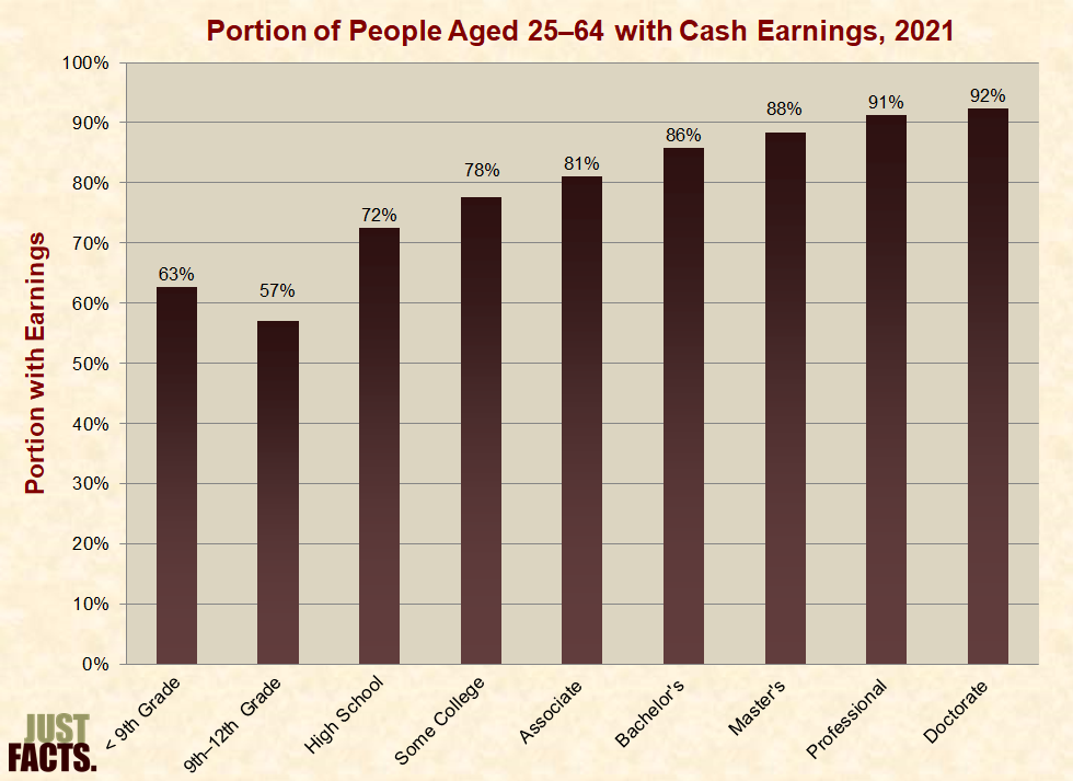
* In 2021, the average reported cash earnings of U.S. residents aged 25–64 with different levels of formal education varied as follows:

* In 2021, 79% of U.S. residents aged 25–64 reported having at least some cash earnings, and 21% did not report any cash earnings. For varying levels of education, the rates varied as follows:
* In 2021, the top-10 highest-paying occupations were all in the medical or dental fields.[460]
* For more facts about education and income, visit Just Facts’ research on education.
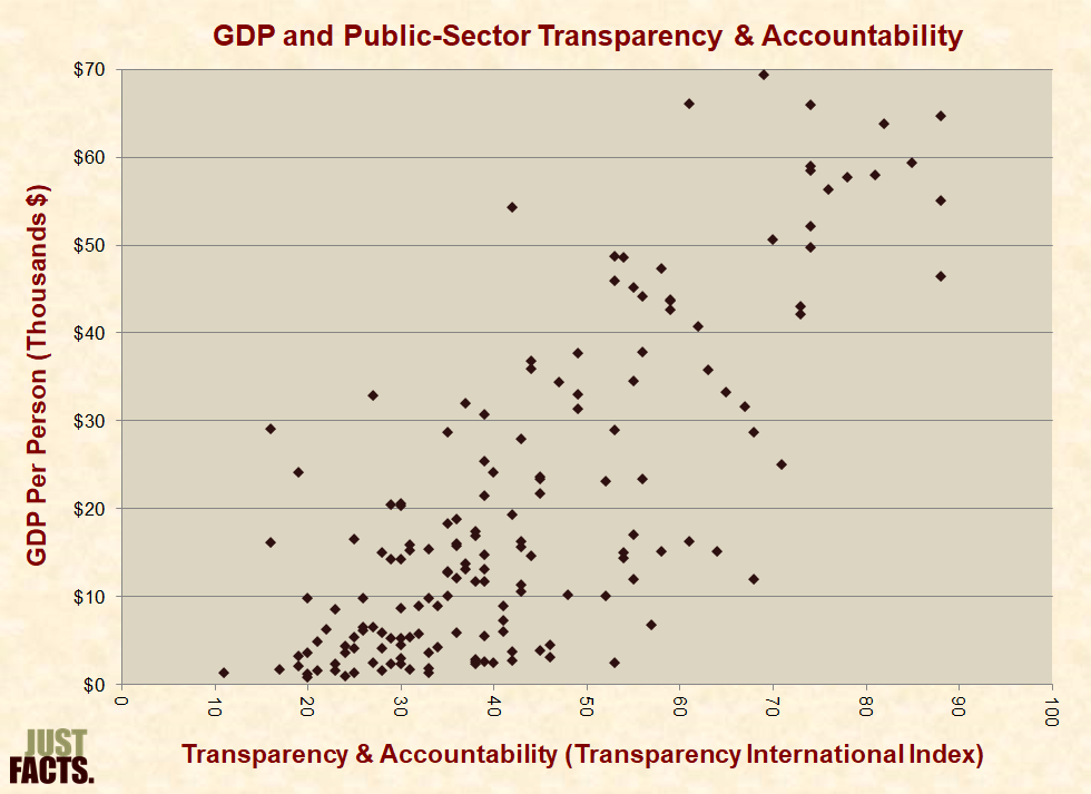
* In 2011, the EPPI-Centre at the University of London published a systematic review of 115 corruption studies which found that “corruption has negative and statistically significant effects on [economic] growth—directly and indirectly.”[461] [462]
* Gross Domestic Product (GDP) is the most common measure of a nation’s economic output.[463] It measures the value of all “goods and services produced within a country’s geographic borders.”[464]
* Per the textbook Microeconomics for Today (and other academic sources):
* Based on data from 170 countries, GDP per person is generally higher in countries with greater public-sector transparency and accountability:
* Nations have three primary types of resources or wealth:
* In 2006, the World Bank analyzed the capital resources of 118 nations and found that the wealth of most nations is mainly comprised of intangible capital. In about 85% of these countries, intangible capital accounted for more than half of their wealth.[475] Per the study:
* In 2005, the capital resources of nations with the highest and lowest wealth per person varied as follows:
|
Total Wealth Top and Bottom 10 Countries, 2005 |
|||||
|
Rank |
Country |
Wealth Per Person (PPP) |
Capital |
||
|
Natural |
Produced |
Intangible |
|||
|
Top 10 Countries |
|||||
|
1 |
Luxembourg |
$779,601 |
$5,805 |
$203,387 |
$570,409 |
|
2 |
Kuwait |
$765,219 |
$618,083 |
$168,548 |
–$21,412 |
|
3 |
United States |
$734,195 |
$13,692 |
$99,137 |
$621,367 |
|
4 |
United Arab Emirates |
$728,889 |
$291,256 |
$175,427 |
$262,207 |
|
5 |
Brunei Darussalam |
$657,376 |
$1,087,550 |
$438,724 |
–$868,898 |
|
6 |
Norway |
$616,547 |
$82,291 |
$136,760 |
$397,496 |
|
7 |
Iceland |
$593,380 |
$7,730 |
$85,959 |
$499,690 |
|
8 |
Singapore |
$555,934 |
$4 |
$183,775 |
$372,155 |
|
9 |
Switzerland |
$543,986 |
$7,511 |
$132,137 |
$404,337 |
|
10 |
Canada |
$537,878 |
$36,665 |
$89,182 |
$412,031 |
|
Bottom 10 Countries |
|||||
|
142 |
Ethiopia |
$13,876 |
$4,406 |
$1,272 |
$8,198 |
|
143 |
Sierra Leone |
$13,061 |
$4,110 |
$758 |
$8,194 |
|
144 |
Niger |
$12,312 |
$3,767 |
$1,017 |
$7,529 |
|
145 |
Chad |
$12,078 |
$10,205 |
$2,878 |
–$1,005 |
|
146 |
Liberia |
$10,631 |
$6,702 |
$454 |
$3,475 |
|
147 |
Guinea-Bissau |
$10,464 |
$5,010 |
$1,456 |
$3,998 |
|
148 |
Mozambique |
$9,807 |
$2,115 |
$1,199 |
$6,492 |
|
149 |
Burundi |
$9,388 |
$10,840 |
$666 |
–$2,118 |
|
150 |
Malawi |
$9,261 |
$2,916 |
$1,315 |
$5,030 |
|
151 |
Congo, Dem. Rep. |
$5,127 |
$3,309 |
$414 |
$1,403 |
* From 1940 to 2022, the portion of unmarried or nonfamily households in the U.S. rose from 24% to 53%:
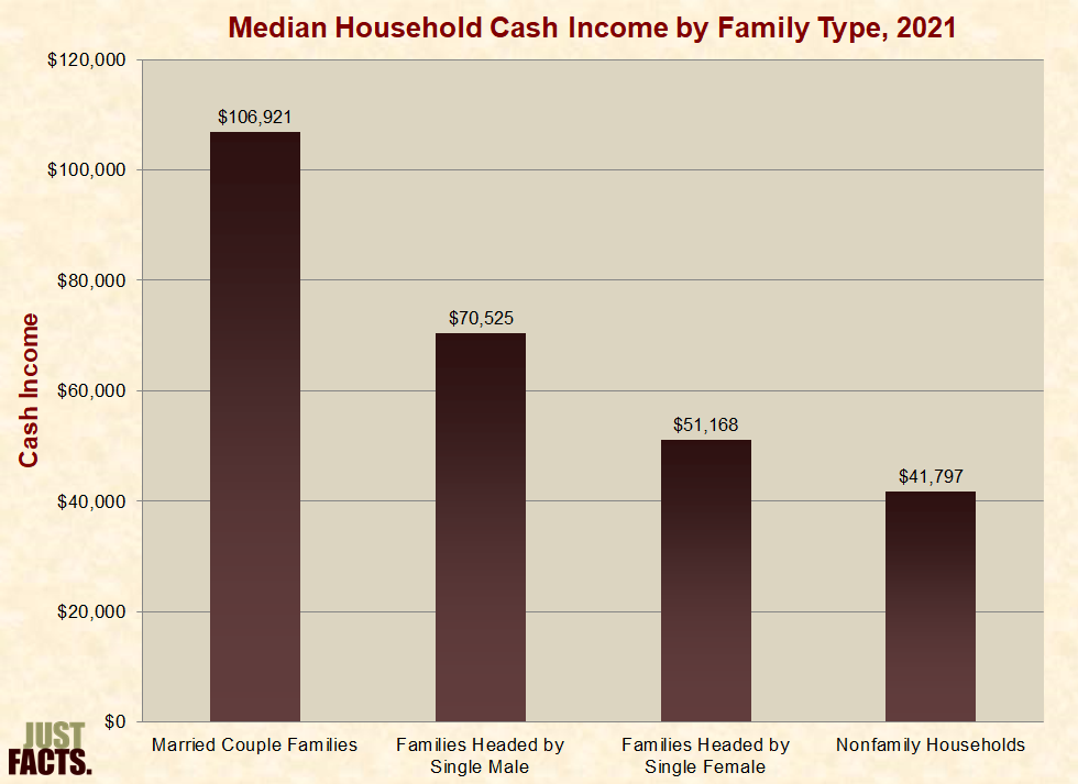
* In 2021, the reported median household cash income for U.S. households with different marital statuses varied as follows:
* In 2011, the reported median cash income of U.S. households with children:
* From 1960 to 2011, the share of single mothers who have never married rose from 4% to 44%.[484]
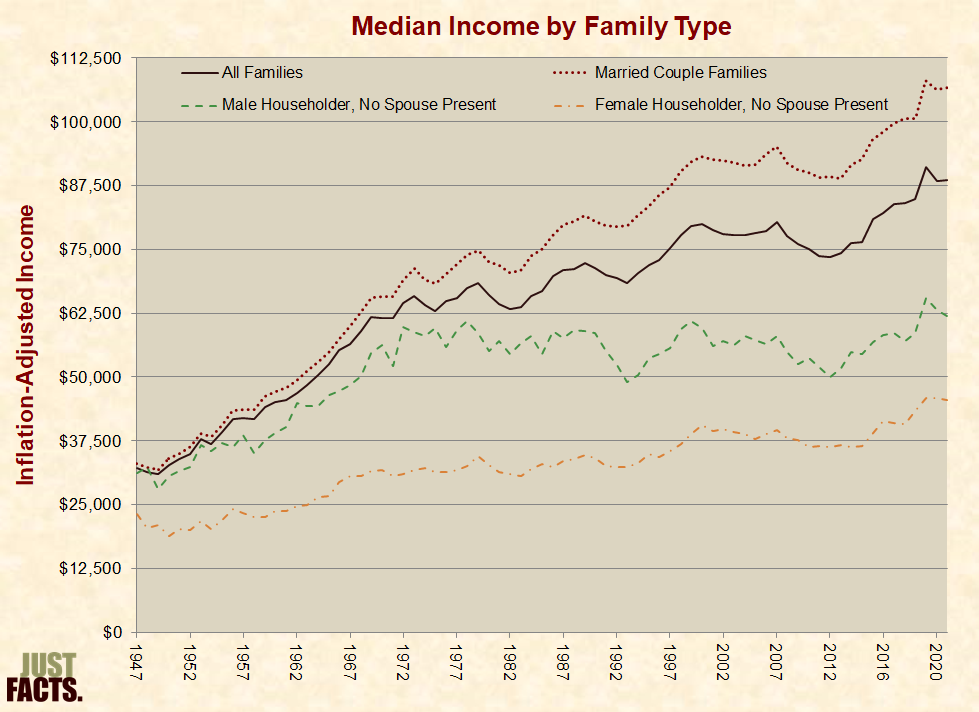
* From 1949 to 2021 the reported median inflation-adjusted cash income of married-couple families in the U.S. rose by 3.2 times. The change in income for other types of families varied as follows:
* In 2021, full-time, year-round female workers reportedly earned median cash wages of $49,263. This was 23% less than the $60,428 earned by males.[487]
* During his 2014 State of the Union address, President Barack Obama stated:
* Obama’s statement does not account for the following factors that pertain to “equal pay” and “equal work”:
* Various studies that have attempted to account for some (but not all) of the factors above have found:
* Per a 2009 analysis of gender wage studies conducted for the U.S. Department of Labor by CONSAD Research Corporation:
* In 2021, the median reported household cash incomes of different races and ethnicities in the U.S. varied as follows:
|
Median Household Cash Income |
|
|
Race / Ethnicity |
Median Income |
|
Asian |
$101,418 |
|
White |
$74,262 |
|
Hispanic |
$57,981 |
|
Black |
$48,297 |
|
All Groups |
$70,784 |
* In 2021, the formal education levels of U.S. residents over age 25 with different races and ethnicities varied as follows:
|
Race / Ethnicity |
Formal Education |
|||
|
No High School Diploma |
High School |
Some College |
Bachelor’s or Higher |
|
|
Asian |
12% |
14% |
17% |
56% |
|
White |
7% |
26% |
29% |
38% |
|
Black |
12% |
31% |
32% |
25% |
|
Hispanic |
28% |
28% |
25% |
20% |
* In 2021, the median reported cash earnings of full-time workers in the U.S. aged 25 and older with different levels of formal education, races, and ethnicities varied as follows:
|
Race / Ethnicity |
Median Earnings (Thousands $) |
|
|
High School[511] |
Bachelor’s or Higher[512] |
|
|
Asian |
$41 |
$95 |
|
White |
$46 |
$81 |
|
Black |
$39 |
$66 |
|
Hispanic |
$41 |
$70 |
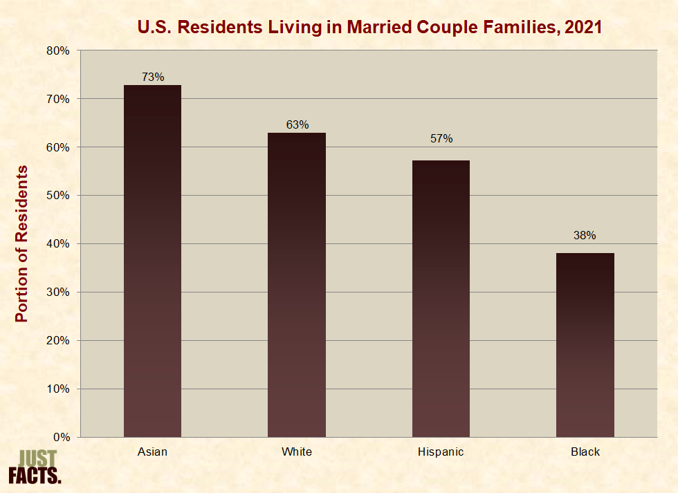
* In 2021, the portion of U.S. residents living in married couple families ranged from 73% for Asians to 38% for blacks:
* In 2021, the median reported household cash incomes for U.S. households of different races, ethnicities, and marital or family statuses were as follows:
|
Race / Ethnicity |
Median Household Cash Income (Thousands $) |
|||
|
Type of Family Household |
||||
|
Married Couple |
Single Male |
Single Female |
Nonfamily |
|
|
Asian |
$131 |
$92 |
$72 |
$59 |
|
White |
$107 |
$72 |
$55 |
$43 |
|
Black |
$90 |
$58 |
$41 |
$34 |
|
Hispanic |
$77 |
$66 |
$45 |
$40 |
|
All Groups |
$107 |
$71 |
$51 |
$42 |
* For more facts about race and income, visit Just Facts’ research on racial issues.
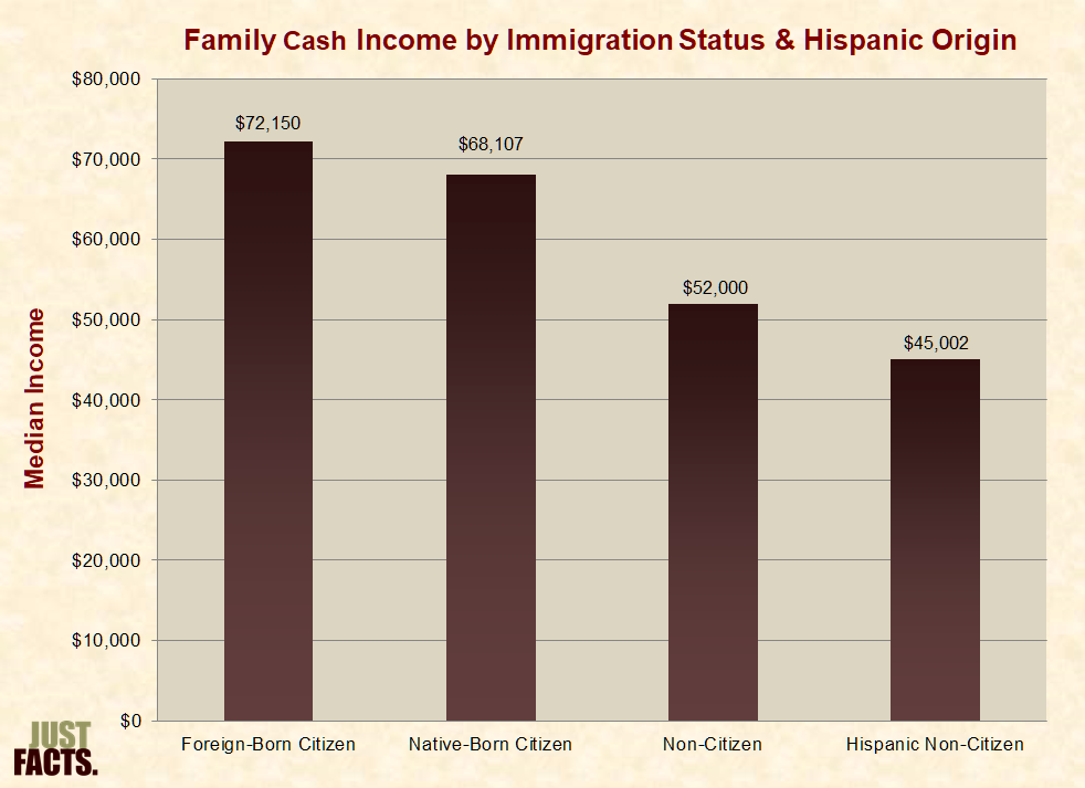
* In 2021, the reported median cash income of families living in the U.S. was $91,162. This varied by immigration status and Hispanic origin as follows:
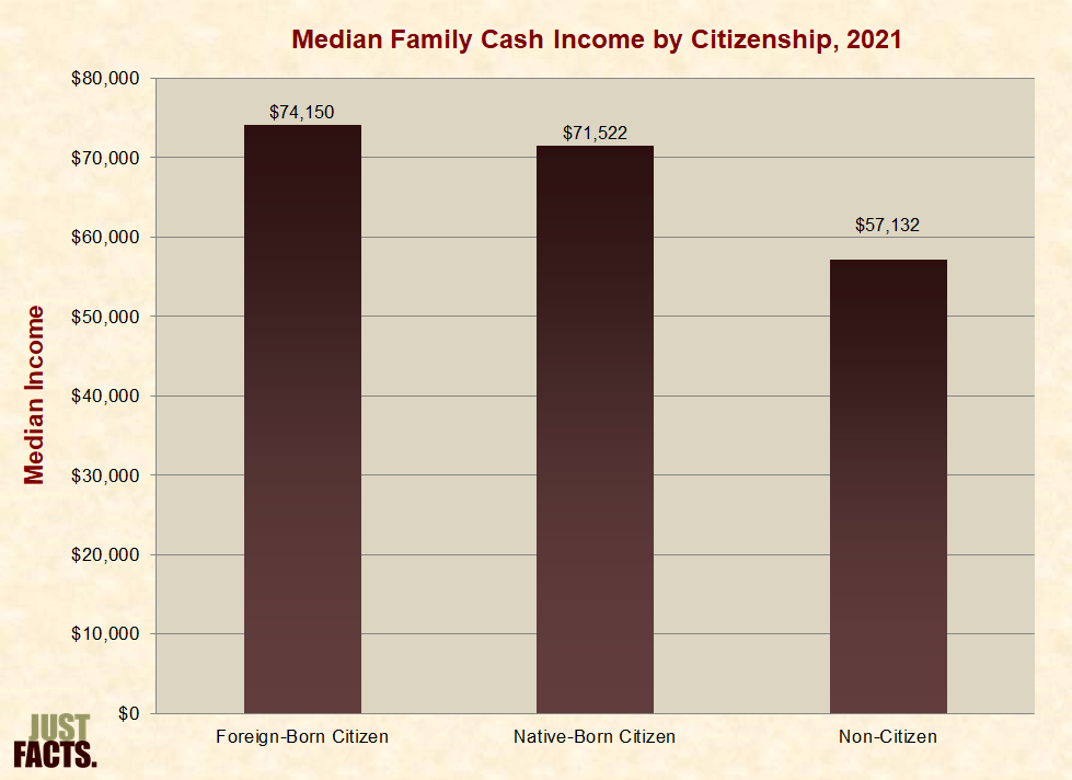
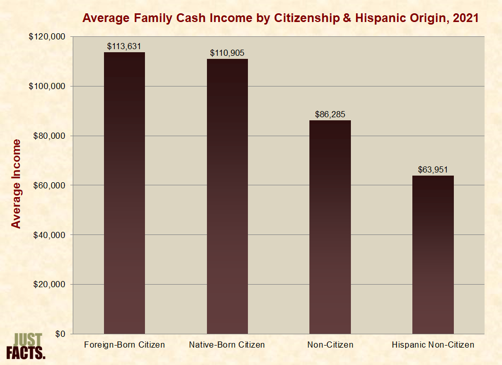
* In 2021, the reported average cash income of families living in the U.S. was $109,299.[525] [526] [527] This varied by immigration status and Hispanic origin as follows:
* In 2017, the reported median cash income of families living in the U.S. was $67,123. This varied by immigration status and Hispanic origin as follows:
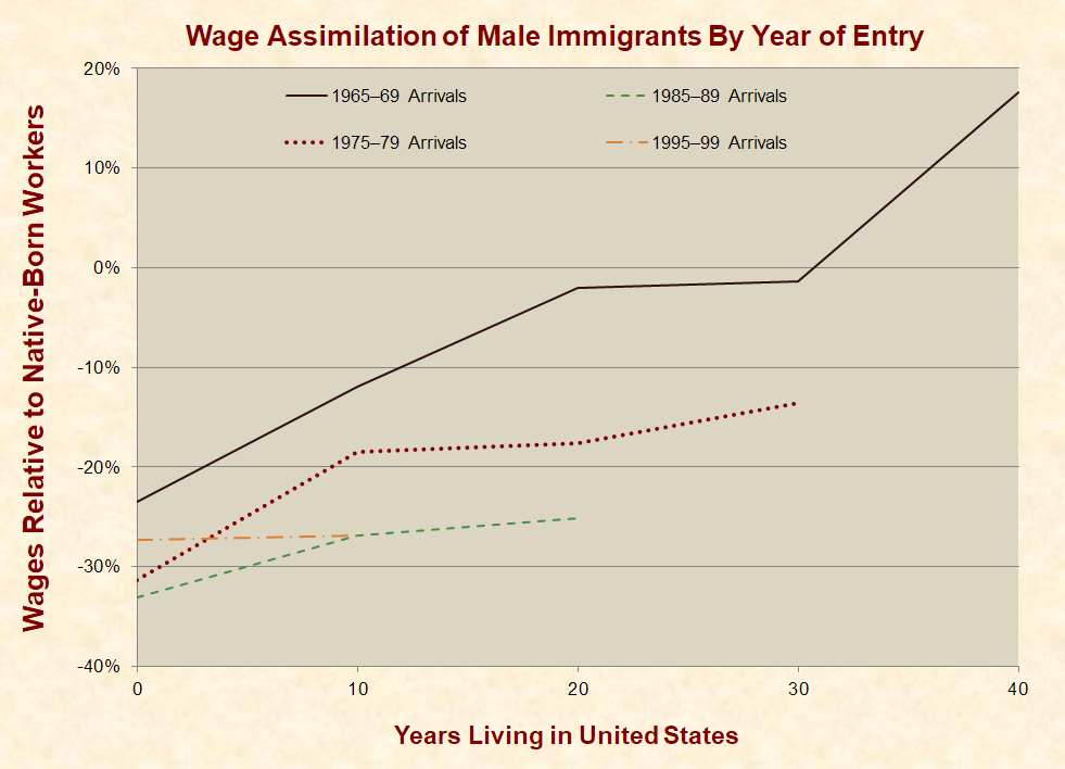
* Male immigrants who arrived in the U.S. during:
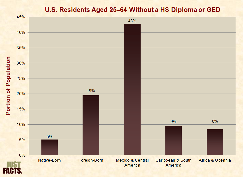
* In 2022, 43% of Mexican and Central American immigrants aged 25–64 did not have a high school diploma or GED, as compared to 5% of people born in the U.S. in the same age group. The rates for other groups were as follows:
* A 2014 study by the Brookings Institution found that:
* For more facts about immigration and income, visit Just Facts’ research on immigration.
* One of the key factors that impact nations’ standards of living is their average hours of work per person.[539]
* Unpaid work—such as caring for children, cooking, and cleaning—increases standards of living, but it is often not recorded in standard economic measures.[540] [541] Per an academic book published by Stanford University Press:
* In 2022, the employment status of the total U.S. civilian, non-institutionalized population was as follows:
* In 2022, the employment status of the U.S. civilian, non-institutionalized population aged 16 years and over was as follows:
* In 2022, the employment status of the U.S. civilian, non-institutionalized population aged 25–54 was as follows:
* In 2021, 16% of adults earned income from occasional informal work.[546]
* Per the Congressional Budget Office:
* The labor force, as defined by the Bureau of Labor Statistics, includes all people who are “either working or actively seeking work.” The potential labor force used by the Bureau to determine the labor force participation rate includes:
* In 2022, men aged 35–44 had a labor force participation rate of 90%. This was the highest rate of all age and gender groups, which varied as follows:
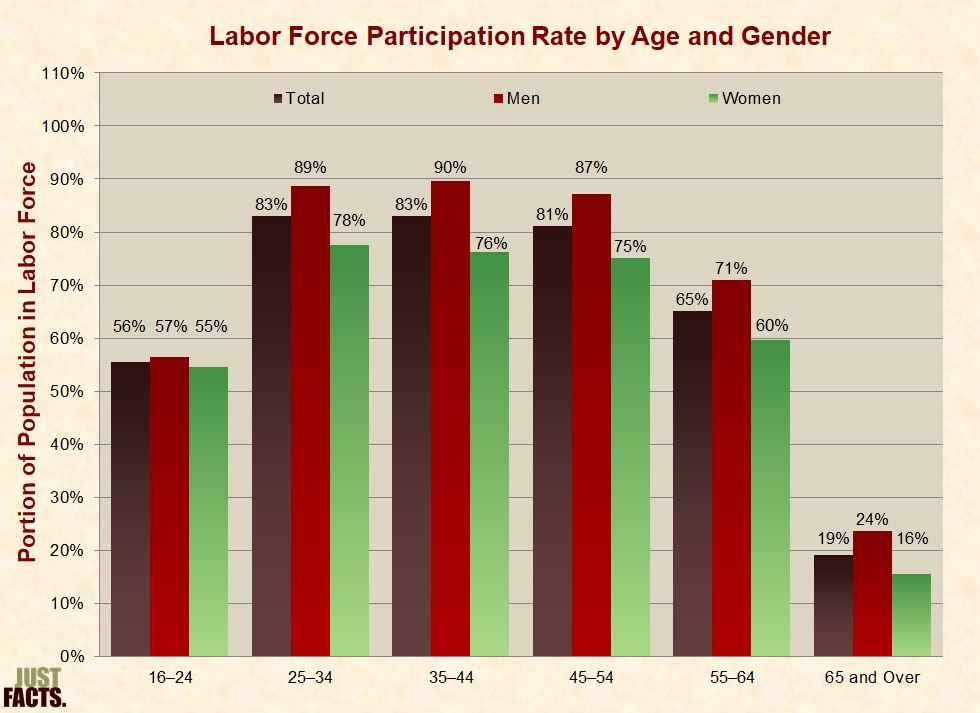
* From 1976 to 2022, the portion of men in their prime working years (25–54) who were not in the labor force increased by 96%.[551] [552]
* Current labor force participation rates for men of all age groups are lower than they were in 1948, while the opposite is true for women:

* As defined by the U.S. Bureau of Labor Statistics, “employed” people are those who, over the course of a week:
* “Unemployed” people are those who are not working but are “available for work” and:
* The federal unemployment rate is determined by dividing the number of unemployed people by the number of people in the labor force.[556] The labor force does not include:
* From 1947 to 2022, the annual unemployment rate averaged 5.7%, varying from a low of 2.9% in 1953 to a high of 9.7% in 1982. In 2022, it was 3.6%:

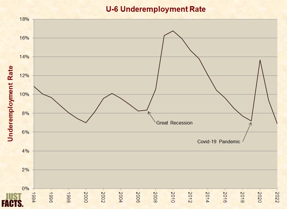
* “Underemployment” is a wider measure of idle potential labor than unemployment. The broadest measure of underemployment published by the U.S. Bureau of Labor Statistics is called “U-6,” which includes:
* From 1994 to 2022, the annual underemployment rate averaged 10.3%, varying from a low of 6.9% in 2022 to a high of 16.7% in 2010. In 2022, it was 6.9%:
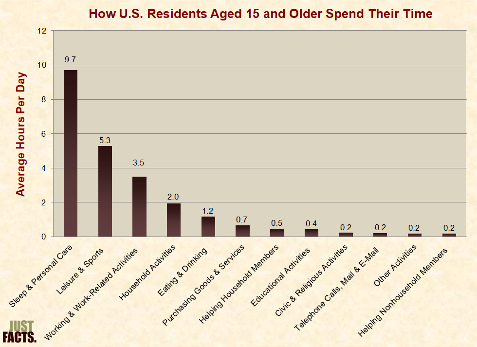
* During 2021, U.S. civilian residents aged 15 and over spent an average of 51% more time on leisure and sports than on paid work and work-related activities:
* During 2021, the U.S. residents of different age groups spent the following hours per day on various activities:
|
Average Hours Per Day Spent on Activities by Age Range |
||||||||
|
Activity |
15–19 |
20–24 |
25–34 |
35–44 |
45–54 |
55–64 |
65–74 |
75+ |
|
Sleep & Personal care |
10.8 |
9.9 |
9.7 |
9.4 |
9.4 |
9.5 |
9.7 |
9.9 |
|
Eating & drinking |
1.1 |
1.2 |
1.1 |
1.1 |
1.2 |
1.3 |
1.3 |
1.4 |
|
Household activities |
0.7 |
1.2 |
1.8 |
1.9 |
2.0 |
2.2 |
2.7 |
2.6 |
|
Purchasing goods & services |
0.5 |
0.7 |
0.6 |
0.6 |
0.7 |
0.7 |
0.8 |
0.7 |
|
Caring for & helping household members |
0.1 |
0.2 |
0.9 |
1.2 |
0.4 |
0.1 |
0.1 |
0.1 |
|
Caring for & helping non-household members |
0.1 |
0.1 |
0.1 |
0.1 |
0.2 |
0.4 |
0.3 |
0.2 |
|
Working & work-related activities |
1.3 |
3.9 |
4.5 |
5.1 |
5.0 |
3.8 |
1.3 |
0.3 |
|
Educational |
3.0 |
1.5 |
0.3 |
0.1 |
0.0 |
0.1 |
–2 |
0.0 |
|
Organizational, civic, & religious activities |
0.2 |
0.1 |
0.1 |
0.2 |
0.2 |
0.3 |
0.4 |
0.4 |
|
Leisure & sports |
5.7 |
4.9 |
4.5 |
3.9 |
4.5 |
5.4 |
6.9 |
7.7 |
|
Telephone calls, mail, & e-mail |
0.4 |
0.2 |
0.2 |
0.1 |
0.2 |
0.2 |
0.3 |
0.3 |
|
Other activities not elsewhere classified |
0.2 |
0.2 |
0.2 |
0.2 |
0.2 |
0.2 |
0.2 |
0.3 |
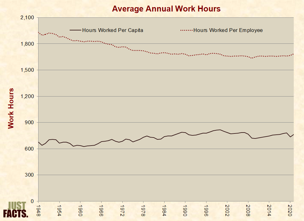
* In 1890, U.S. manufacturing laborers worked an average of 60 hours per week,[571] as compared to 40 hours in 2022.[572]
* In the U.S. from 1948 to 2021, the average annual work hours per employee declined by 13%.[573] Over this period, work hours per employee and per person varied as follows:
* In 2021, full-time workers averaged 8.2 hours of work per day on the days that they worked. This figure was higher on weekdays (8.5 hours) than on weekends or holidays (5.9 hours).[575]
* A 2011 study published by U.S. Bureau of Labor Statistics found that:
* Some of the primary factors that determine employee compensation are:[579]
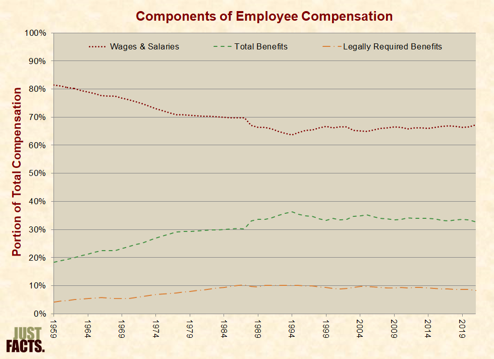
* Per the U.S. Department of Labor, “In the final four decades of the 20th century, employee compensation, as measured by employer costs, has undergone dramatic shifts” from cash to benefits. Many of these benefits are “legally required” by government, such as Social Security and Medicare.[590]
* Government mandates that force employers to pay for programs like Social Security, Medicare, and the Affordable Care Act (ACA) suppress the wages and salaries of employees. Per the:
* From 1959 to 2021, the portion of blue collar worker compensation consisting of:
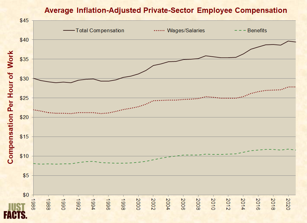
* Adjusted for inflation, the average hourly compensation of private-sector employees (including wages, salaries, and benefits) rose by 31% between 1986 and 2021:
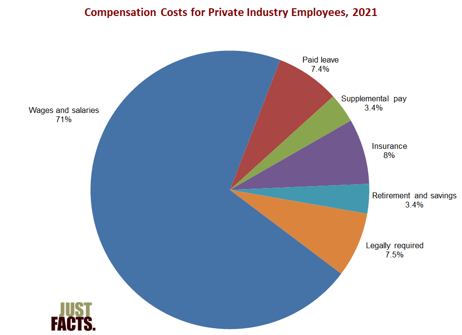
* In 2021, the components of compensation for private industry employees were as follows:
* Adjusted for inflation, average hourly employee compensation rose at the following rates over the time periods below:
|
Inflation-Adjusted Hourly Cost Growth of Employee Compensation |
||
|
Category |
Private Sector |
State and Local |
|
Wages & Salaries |
27% |
22% |
|
Benefits |
43% |
72% |
|
Total |
31% |
37% |
* In 2022, federal, state, and local governments spent $2.21 trillion on employee compensation. This amounts to an average of $17,016 from every household in the United States.[604] [605] [606] [607] [608] [609]
* In 2022, government workers accounted for 15% of all employees in the United States.[610]
* Adjusted for inflation, the average hourly compensation of government employees (including wages, salaries, and benefits) rose by 31% between 1991 and 2021:

* In 2017, the Congressional Budget Office published a study comparing the compensation of full-time, year-round private sector workers to non-postal, civilian, federal workers in 2011 to 2015. The study accounted for education, occupation, work experience, geographic location, employer size, and various demographic characteristics. The study found that:
|
Federal Employee Compensation Premiums Relative to Private Sector |
|||
|
Formal Education |
Wages |
Benefits |
Total |
|
High School Diploma or Less |
34% |
93% |
53% |
|
Some College |
22% |
80% |
39% |
|
Bachelor’s Degree |
5% |
52% |
21% |
|
Master’s Degree |
–7% |
30% |
5% |
|
Professional Degree or Doctorate |
–24% |
–3% |
–18% |
|
All Levels of Education |
3% |
47% |
17% |
* Click here for an article from Just Facts about the compensation of federal civilian employees and a broad range of studies about this issue.
* Adjusted for inflation, average hourly employee compensation rose at the following rates over the time periods below:
|
Inflation-Adjusted Hourly Cost Growth of Employee Compensation |
||
|
Category |
Private Sector |
State and Local |
|
Wages & Salaries |
27% |
22% |
|
Benefits |
43% |
72% |
|
Total |
31% |
37% |
* In 2013, the journal Public Administration Research published a study comparing the compensation of full-time workers over 50 years of age in government and private sectors during 2006. The study accounted for wages and pensions but not “employment security, paid vacation, health insurance benefits,” and other types of compensation. It found that:
* In 2010, full-time private industry workers worked an average of 12% more hours per year than full-time state and local government workers. This includes time spent working beyond assigned schedules at the workplace and at home.[615]
* For more facts about government employee compensation, visit Just Facts’ research on unions.
* Minimum wage laws force employers to pay certain employees more than the market rate for their services.[616] [617]
* In 1931, the 71st U.S. Congress and Republican President Herbert Hoover enacted the first federal minimum wage law. It required contractors engaged in federal construction projects in excess of $5,000 dollars to pay workers “not less than the prevailing rate of wages for work of a similar nature in” the area.[618]
* In 1938, the 75th U.S. Congress and Democratic President Franklin D. Roosevelt enacted a law that required all employers to pay a minimum wage to most employees “engaged in commerce or in the production of goods for commerce.”[619]
* The 1938 law set the federal minimum wage at $0.25 per hour. Adjusted for inflation, this is equivalent to $5.30 in 2023 dollars.[620] [621]
* Since 1938, various federal laws have increased the minimum wage more than 20 times. The latest increase, in July of 2009, brought the minimum wage to $7.25 per hour.[622]
* Adjusted for inflation, the federal minimum wage is currently 37% higher than when it was enacted in 1938.[623]
* Federal minimum wage law has exceptions that “apply under specific circumstances to workers with disabilities, full-time students, youth under age 20 in their first 90 consecutive calendar days of employment, tipped employees and student-learners.”[624]
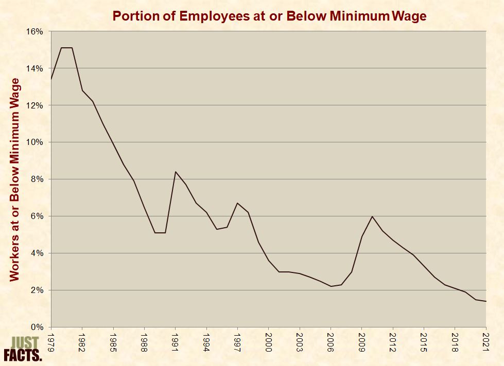
* Excluding tips, commissions, and overtime pay, 1% of all employees in the U.S. were paid at or below the federal minimum wage in 2021. The rates for different age groups varied as follows:
|
U.S. Employees Paid at or Below Minimum Wage |
||
|
Age Group |
Total |
Portion |
|
16 to 19 Years |
4,776,000 |
4% |
|
20 to 24 Years |
10,377,000 |
3% |
|
25 Years and Older |
60,973,000 |
1% |
* Per the U.S. Bureau of Labor Statistics:
* In 2021, part-time hourly employees—those who worked 34 hours or less—accounted for 48% of employees at or below the federal minimum wage.[627]
* The portion of employees at or below federal minimum wage peaked at 15% in 1980 and 1981. It has since varied as follows:
* As of January 1, 2023:
* While noting there is “considerable uncertainty” about the effects of the minimum wage, a 2019 study by the Congressional Budget Office found that increasing the minimum wage by 65%, or from $7.25 per hour to $12, “would boost wages, but it would also increase joblessness, reduce business income, raise prices, and lower total output in the economy.”[631] With regard to families at different income levels, the study estimated that such a law would:
* The same 2019 Congressional Budget Office study estimated that increasing the minimum wage by more than 100%, or from $7.25 per hour to $15 would:
* A 5.2% increase in reported cash income (or $589) would raise the average total income of families below the poverty line by about 1%. This is because reported cash income accounts for about 19% of their total income, while the other 81% is comprised of unreported cash and non-cash government benefits like Food Stamps, Medicaid, housing, and a wide array of other programs.[636] [637] [638] [639]
* Per a 2014 paper by Ph.D. labor economists David Neumark, J.M. Ian Salas, and William Wascher:[640] [641] [642]
* In 2007, the journal Foundations and Trends in Microeconomics published a review of the “new minimum wage research” that examined 102 studies. This review found that:
* In 2015, the Los Angeles Federation of Labor union helped lead an effort to increase the minimum wage in Los Angeles to $15/hour by 2020. After the city council passed the bill, the same labor union lobbied to change it so that companies with union workers would be exempt from the law.[648]
* For more facts about the effects of governments forcing employers to pay wages that are above market rates, visit Just Facts’ research on unions.
* The U.S. Department of Labor regulates overtime pay, which is 1.5 times an employee’s hourly rate for hours worked over forty hours.[649]
* Executive, administrative and professional workers are among those employees who are exempt from overtime pay regulations.[650]
* In the 2000s, three employees brought a class action lawsuit against IBM for withholding overtime pay from workers that IBM considered to be exempt from the regulations. The company settled the lawsuit for $65 million.[651] [652]
* To prevent future lawsuits, IBM converted 7,000 salaried employees into hourly employees and decreased their base pay by 15% to offset the anticipated overtime costs.[653]
* In 2016, the U.S. Department of Labor, then under the leadership of Barack Obama, enacted a regulation to make overtime pay mandatory for workers earning less than $47,476/year. This was double the previous threshold of $23,660.[654] [655] [656]
* Obama’s regulation was scheduled to take effect on December 1, 2016,[657] but a federal judge granted an injunction before it was implemented.[658]
* In 2017, a federal judge appointed by Obama struck down this regulation,[659] and the Trump administration decided to not appeal this ruling.[660]
* Wealth, or net worth, is the value of assets minus debts at a given point in time, while income is “a flow of purchasing power.” [661] [662] [663] [664] [665]
* Assets include items such as:
* Per the Organization for Economic Cooperation and Development and the U.S. Census Bureau:
* Researchers generally consult two primary sources of information for the wealth of U.S. residents: the Federal Reserve’s Survey of Consumer Finances and Internal Revenue Service tax returns. The Congressional Budget Office and the Census Bureau also publish wealth data.[670] [671] [672] [673] [674] These sources have varying strengths and weaknesses:
* Per the Federal Reserve’s Survey of Consumer Finances:
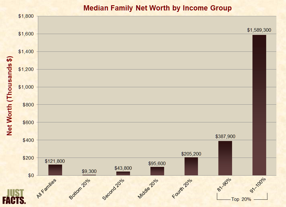
* According to the Federal Reserve’s Survey of Consumer Finances, the median net worth of U.S. families was $121,800 in 2019. The net worth for different income groups varied as follows:
* The inflation-adjusted median net worth of U.S. families increased by 30% from 1989 to 2019. The change in net worth for different wealth groups varied as follows:

* Per a 2017 report by the Federal Reserve:
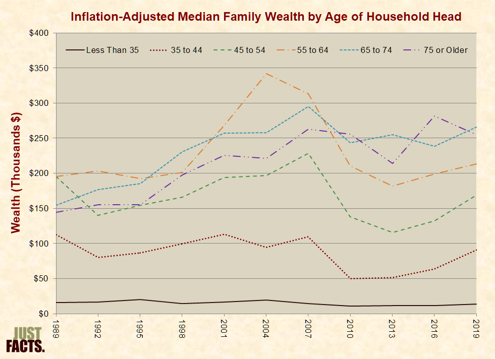
Age
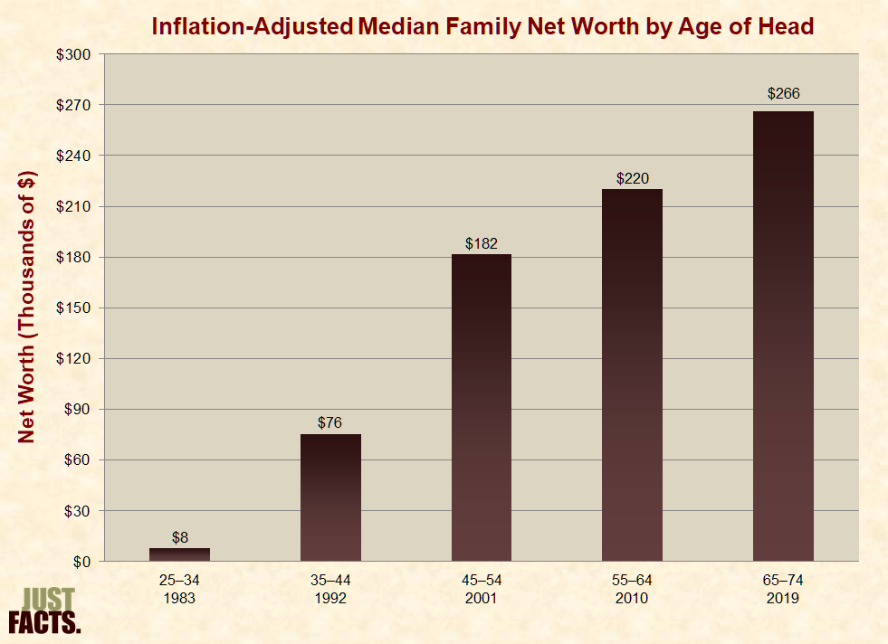
* In 2019, the median wealth of families where the head of household is aged 65 to 74 was 18.2 times that of families under the age of 35:
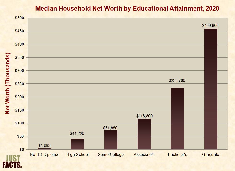
Education
* According to U.S. Census Bureau data, the median net worth of households in which someone had a bachelor’s degree (and no further education) was $233,700 in 2020. The net worth of those with other levels of educational attainment varied as follows:
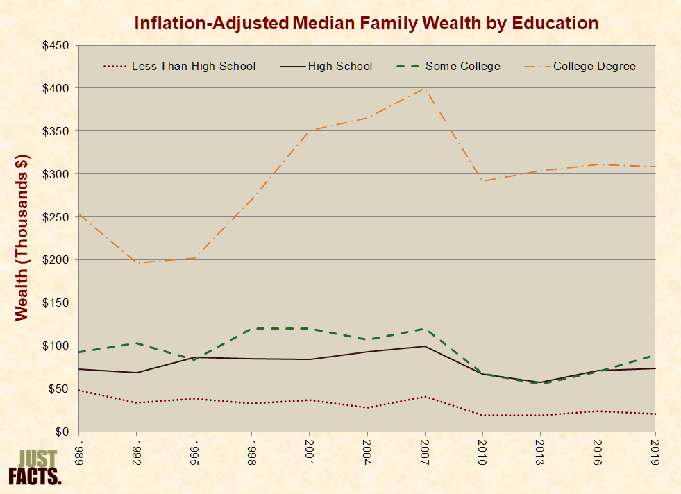
* Federal Reserve data shows that from 1989 to 2019, inflation-adjusted median family wealth:
Race
* The median net worth of U.S. families was $121,800 in 2019. Family net worth by race and ethnicity varied as follows:
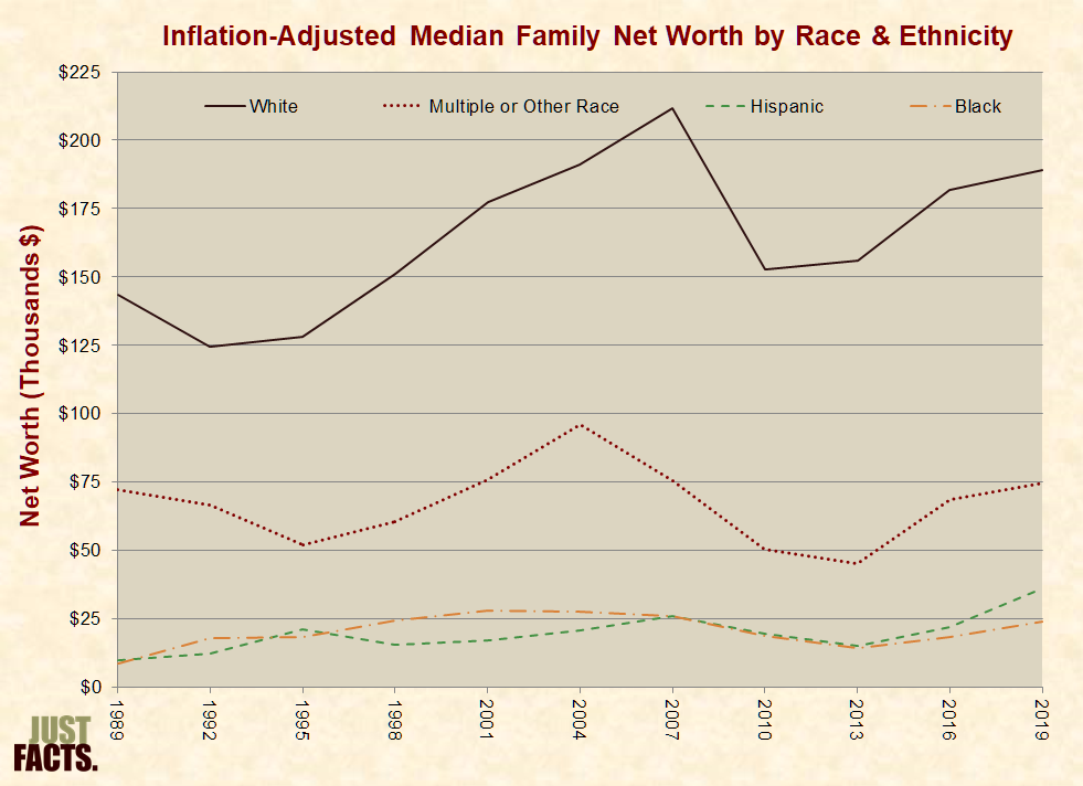
* Data from a 2020 study by the Federal Reserve show that inheritances account for 11% of the median wealth gap between blacks and whites.[698]
Family Structure
* The median net worth of U.S. families was $121,800 in 2019. Net worth by family structure varied as follows:

* In 2021, 75% of working adults reported having “at least some retirement savings,” while about 25% said they had none.[701]
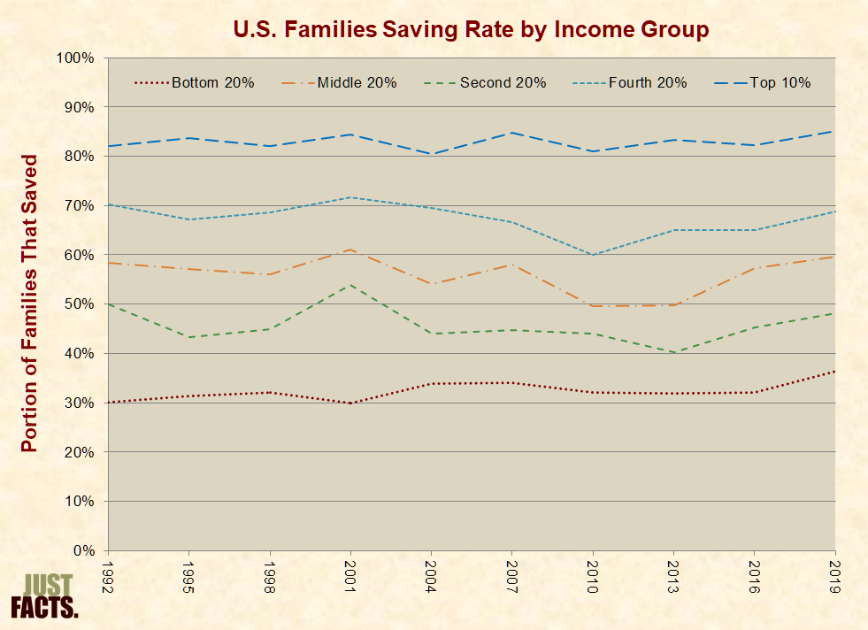
* In 2019, 36% of low-income families were saving some of their income, as compared to 60% of middle-income families. From 1992 to 2019, the portion of families who saved varied as follows:
* Per the Congressional Budget Office:
* The Congressional Budget Office and the Survey of Consumer Finances provide “a series of snapshots of family wealth” rather than “information about changes in the wealth of particular families over time.”[704]
* It is possible to approximate changes in the net worth of particular families over time. For example, many of the 25–34 year-olds interviewed for the 1983 Survey of Consumer Finances were aged 35–44 in the 1992 survey (notwithstanding the deceased and migrants). From 1983 to 2019, this group of families increased their median inflation-adjusted net worth by 33 times:
* In 2018, the Journal of Human Development and Capabilities published a paper that found:
* Per Ph.D. economist Martin Feldstein, professor of economics at Harvard University and President Emeritus of the National Bureau of Economic Research:[708]
* Middle-income U.S. workers are hindered from saving because they are forced to contribute 15.3% of their paychecks to social insurance taxes.[710] If these workers saved and invested one-fifth of these taxes during their careers, each retired worker would have an additional $199,000 to $764,000 in savings today.[711]
* A study published by the University of Chicago Press in 2002 found that Social Security:
* Per the U.S. Federal Deposit Insurance Corporation (FDIC):
* In 2019, 18% of U.S. families’ access to credit was constrained due to denial (11%) and the fear of denial (13%).[715]
* In 1999, Freddie Mac—a government-sponsored enterprise that is tasked to “promote affordable housing”—published a study that measured the rates of “bad credit” among Americans of different races. As defined by the study, people with “bad credit” were those over the past two years who were more than 30 days late paying two bills, more than 90 days late paying one bill, or had a bankruptcy, lien, or judgment. The study, which was based on a scientific sample of 80,000 people, showed that upper-middle income blacks had a higher rate of bad credit than lower-income Asians and whites. For example:
* Per a 2017 study in the Journal of Behavioral and Experimental Finance, the “ability to control impulses is undoubtedly a key factor for long-term success in many areas of life.”[718]
* A 2015 paper by scholars from the International Monetary Fund and the European Central bank found that households who:
* A 2020 study by the Federal Reserve found that 30% of white families in the U.S. have received an inheritance. Adjusted for inflation into 2019 dollars, the median value of these inheritances was $88,500. For various races and ethnicities, inheritances are as follows:
|
Inheritances |
White |
Black |
Hispanic |
Other |
|
Portion Who Received |
30% |
10% |
7% |
18% |
|
Median Value (2019 dollars) |
$88,500 |
85,800 |
$52,200 |
$59,400 |
* Data from the same study show that inheritances account for 11% of the median wealth gap between blacks and whites.[721]
* Per the Department of Housing and Urban Development:
* Some of the downsides of owning a home can include:
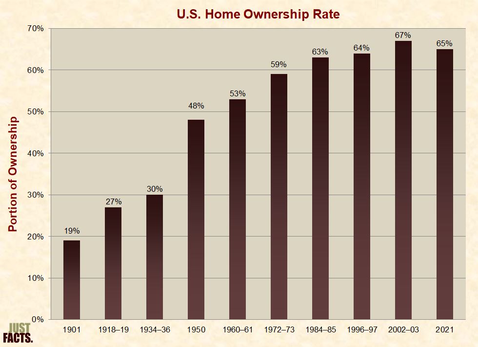
* In 2021, 65% of U.S. households owned their home. Since 1901, home ownership rates have varied as follows:
* Poverty can be measured in absolute or relative terms. Relative poverty is based on comparisons to people living in certain nations or areas, while absolute poverty is based on stable benchmarks.[730] For example:
* Governments originally measured poverty based on people’s consumption of goods and services. They now measure poverty based on people’s “money income” because it is easier for people to report this.[734] [735] [736] [737] Money income:
* The official U.S. poverty rate:
* With regard to the exclusion of noncash benefits from money income:
* With regard to the underreporting of cash income on government household surveys:
* In 2010 (latest data), the poorest 20% of households reported an average of $11,034 in pre-tax money income per household, while they consumed an average of $57,049 of goods and services per household—or 5.2 times their reported money income:
* The official poverty thresholds were developed in 1963–1964 by an economist at the Social Security Administration named Mollie Orshansky. In 1969, the White House Office of Management & Budget made them the formal standard. Per Orshansky:
* The U.S. government uses two “slightly different” poverty benchmarks:
* The Census Bureau poverty thresholds “do not vary geographically, but they are updated for inflation using the Consumer Price Index.”[781]
* Per the Department of Health and Human Services, its:
* In 2022, the Census Bureau poverty thresholds and Health and Human Services poverty guidelines for families or households of different sizes varied as follows:
|
2022 Poverty Measures |
||
|
Family/Household |
Census Thresholds* |
HHS Guidelines† |
|
1 Adult, No Children |
$15,225 |
$13,590 |
|
1 Adult, 1 Child |
$20,172 |
$18,310 |
|
1 Adult, 2 Children |
$23,578 |
$23,030 |
|
1 Adult, 3 Children |
$29,782 |
$27,750 |
|
2 Adults, No Children |
$19,597 |
$18,310 |
|
2 Adults, 1 Child |
$23,556 |
$23,030 |
|
2 Adults, 2 Children |
$29,678 |
$27,750 |
|
2 Adults, 3 Children |
$34,926 |
$32,470 |
|
* Householder under age 65 |
||
|
† 48 Contiguous States and the District of Columbia |
||
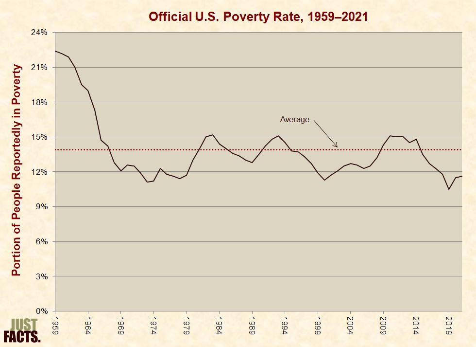
* In 2021, the official U.S. poverty rate was 11.6%, representing 38 million people in poverty.[785]
* From 1959 to 2021, the portion of the U.S. population with reported cash income at or below the official federal poverty line ranged from 22.4% to 10.5%, with an average of 13.9%:
* In 2021, the portion of the U.S. population with reported cash income at or below:
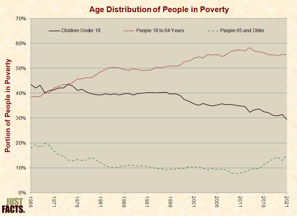
* In 2021, adults aged 18–64 accounted for 55% of people reportedly in poverty. Children under the age of 18 and people above 65 years comprised 29% and 15%, respectively. From 1966 to 2021, the portion of the U.S. population reportedly in poverty varied by age as follows:
* “Means-tested welfare” programs—commonly called “welfare”—provide cash and other benefits to people with incomes and/or assets below certain thresholds. Examples of such include:
* In 2015, the U.S. Government Accountability Office identified 82 federal means-tested welfare programs.[795]
* Seven of the 10 largest federal means-tested welfare programs are “mandatory.”[796] [797] This means they are permanently funded and can spend money without Congress and the president passing new laws. In contrast, Congress and the president typically fund “discretionary” programs for one year at a time.[798] [799]
* In 2020, the federal government spent $869 billion on mandatory means-tested welfare programs, amounting to 81% of all spending “on benefits and services for people with low income.”[800]
* Per the U.S. Government Accountability Office:
* Various government agencies use the Department of Health and Human Services poverty guidelines—or multiples of them—to determine eligibility for at least 31 means-tested programs.[804] Eligibility for the programs below is based on the applicant’s reported income being at or under the following percentages of the HHS poverty guidelines:
* The following programs use other criteria instead of the Health and Human Services guidelines:
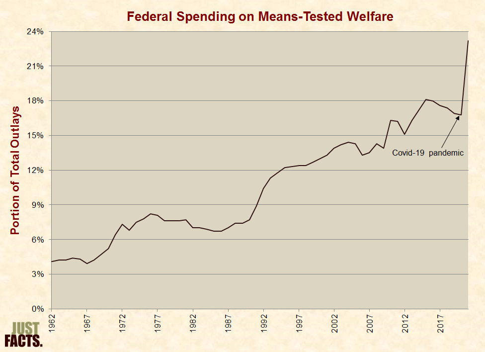
* In 2021—amid the Covid-19 pandemic,[811] [812] the federal government spent $1.6 trillion on means-tested welfare.[813] [814] This amounts to:
* From 1962 to 2021, spending on means-tested welfare increased from 4% of all federal outlays to 23%:
NOTE: When interpreting the facts in this section, it is important to realize that correlation does not prove causation. This is because numerous factors can affect societal outcomes like poverty, and there is frequently no objective way to identify, measure, and determine the interplay between all of them.
* In 2021, the portion of the U.S. population aged 18–64 with incomes reportedly below Census Bureau poverty thresholds varied by work time as follows:
|
People Aged 18–64 in Poverty by Work Time, 2021 |
|
|
Type of Worker |
Portion |
|
Less Than 1 Week of Work |
30% |
|
Less Than Full-Time Year-Round Workers |
12% |
|
All Workers |
5% |
|
Full-Time Year-Round Workers |
2% |
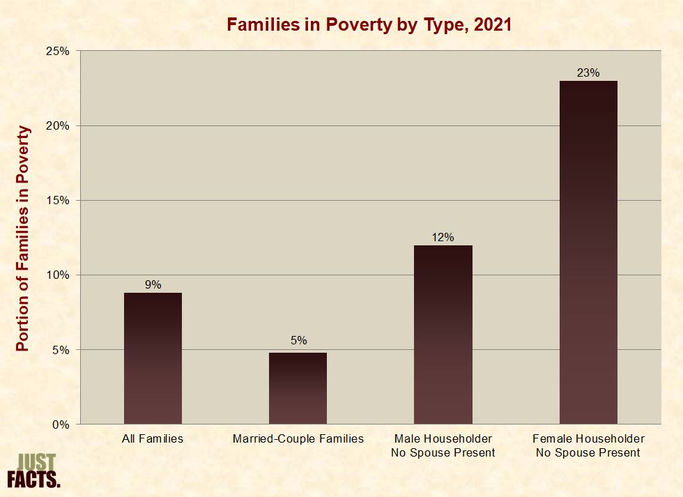
* In 2021, 5% of married-couple families reported incomes below Census Bureau poverty thresholds. The rates for other types of families varied as follows:
* In 2021, the portion of children in families with incomes reportedly below Census Bureau poverty thresholds varied by their family structure as follows:
|
Children in Poverty by Family Structure, 2021 |
|
|
Kind of Family |
Portion |
|
Female Householder |
36% |
|
Male Householder |
18% |
|
Husband–Wife Family |
7% |
* In 2021, the portion of the U.S. population with incomes reportedly below Census Bureau poverty thresholds varied by race as follows:
|
People in Poverty by Race, 2021 |
|
|
Race |
Portion |
|
Black |
20% |
|
Hispanic |
17% |
|
White |
10% |
|
Asian |
9% |
* In 2019—prior to the Covid-19 pandemic—the reported poverty rates for U.S. residents of different races, ethnicities, and marital statuses varied as follows:
|
Race / Ethnicity |
Poverty Rate by Race, Ethnicity, and Marital Status, 2019 |
|||
|
Married, Spouse Present |
Divorced |
Separated |
Never Married |
|
|
White |
6% |
14% |
24% |
13% |
|
Asian |
9% |
13% |
26% |
14% |
|
Black |
9% |
19% |
28% |
21% |
|
Hispanic |
14% |
19% |
34% |
20% |
* In 2021—amid increased government spending on Covid-19 “relief” programs—the reported poverty rates for U.S. residents of different races, ethnicities, and marital statuses varied as follows:
|
Race / Ethnicity |
Poverty Rate by Race, Ethnicity, and Marital Status, 2021 |
|||
|
Married, Spouse Present |
Divorced |
Separated |
Never Married |
|
|
White |
4% |
11% |
12% |
7% |
|
Asian |
7% |
12% |
17% |
11% |
|
Black |
7% |
15% |
16% |
12% |
|
Hispanic |
9% |
13% |
18% |
11% |
* For more facts about poverty and race, visit Just Facts’ research on racial issues.
* In 2021, the portion of the U.S. population aged 18–64 with incomes reportedly below Census Bureau poverty thresholds varied by immigration status as follows:
|
People Aged 18–64 in Poverty by Immigration Status, 2021 |
|
|
Nativity Status |
Portion |
|
Non-Citizen |
17% |
|
Native Born |
10% |
|
Naturalized Citizen |
9% |
* For more facts about poverty and immigration, visit Just Facts’ research on immigration.
* In 2021, the portion of the U.S. population aged 25 and older with incomes reportedly below Census Bureau poverty thresholds varied by educational attainment as follows:
|
People Aged 25 and Older in Poverty by Education, 2021 |
|
|
Educational Attainment |
Portion |
|
No High School Diploma |
27% |
|
High School, No College |
13% |
|
Some College, No Degree |
9% |
|
Bachelor’s Degree or Higher |
4% |
* For more facts about poverty and education, visit Just Facts’ research on education.
* In 2021, the portion of the U.S. population aged 18–64 with incomes reportedly below Census Bureau poverty thresholds varied by disability status as follows:
|
People Aged 18–64 in Poverty by Disability Status, 2021 |
|
|
Disability Status |
Portion |
|
With a Disability |
25% |
|
With No Disability |
9% |
* Per the U.S. Census Bureau:
* Per a 2007 Federal Reserve Board working paper published near the outset of the Great Recession:
* The same Federal Reserve paper states that the increases “in debt–income ratios” make “some households more vulnerable to shocks to” incomes, interest rates, and asset prices.[846]
* Debt can be secured or unsecured.[847] Per the District of Oregon U.S. Bankruptcy Court:
* Some of the consequences of failure to repay unsecured debt are:
* In the fourth quarter of 2022, the average U.S. household owed $144,475 in consumer debt, such as mortgages and credit cards.[850]
* In 2019, 77% of U.S. families had some kind of debt. Among these families, the median debt was $65,000, and:
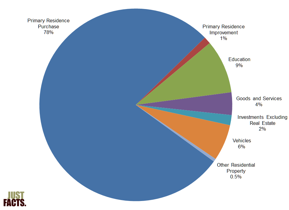
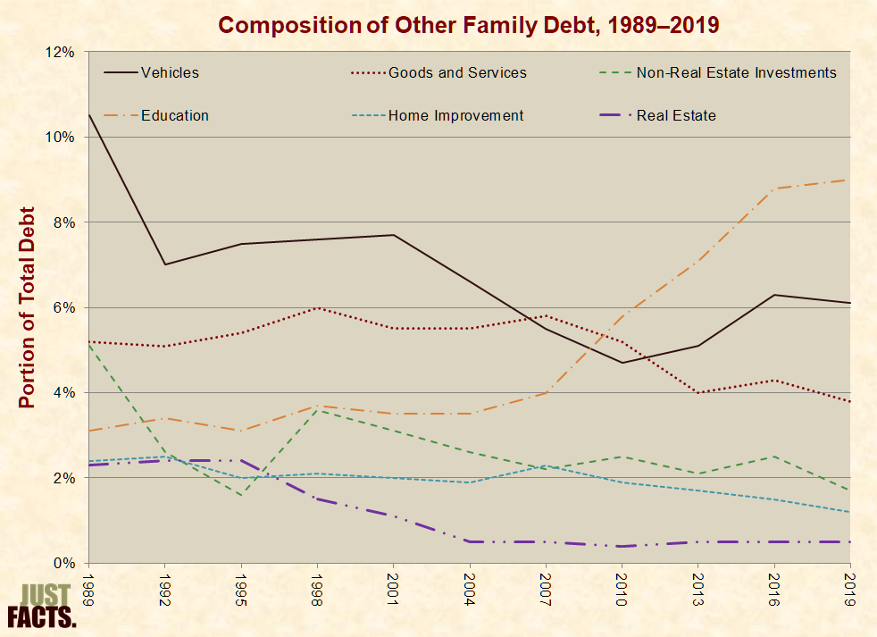
* The most common category of family debt in 2019 was for a primary residence. Other categories varied as follows:
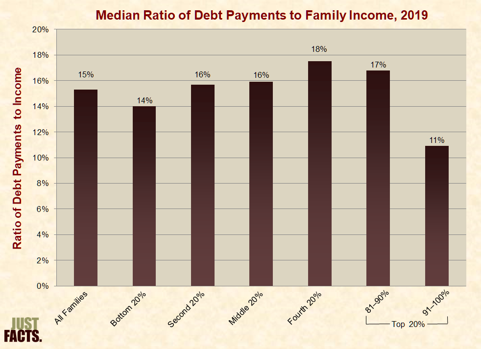
* In 2019, the median ratio of debt payments to family income for families who carried debt was 15%. This varied by family income as follows:
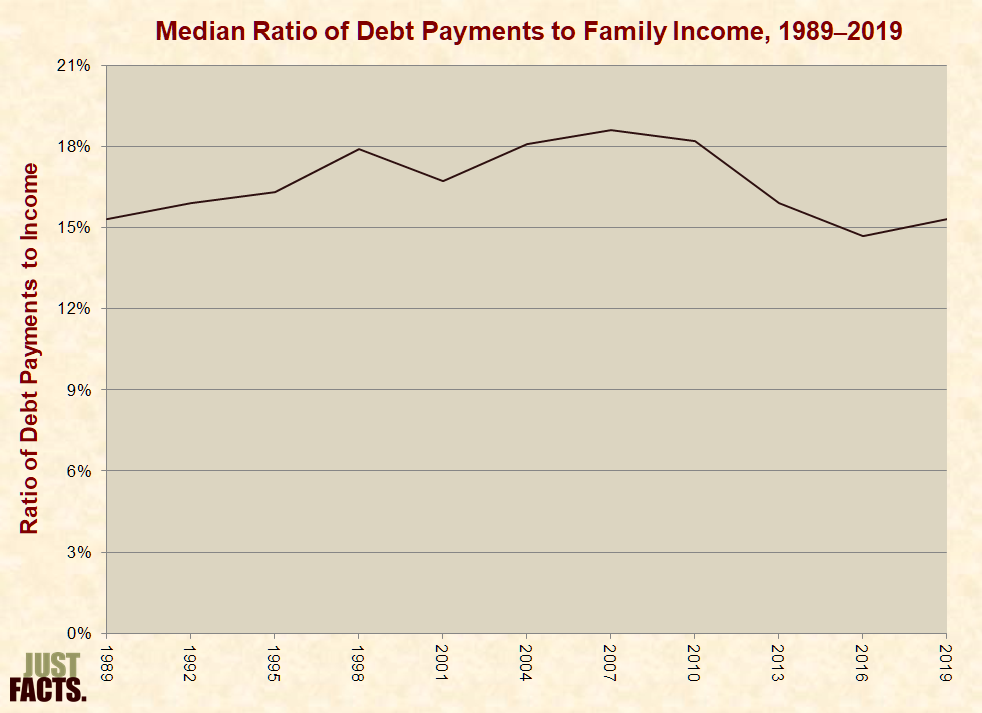
* In 2019, the median ratio of family debt payments was roughly 15%. Since 1989, the ratio has varied as follows:
* In 2016, the Congressional Budget Office reported that during and after the Great Recession:
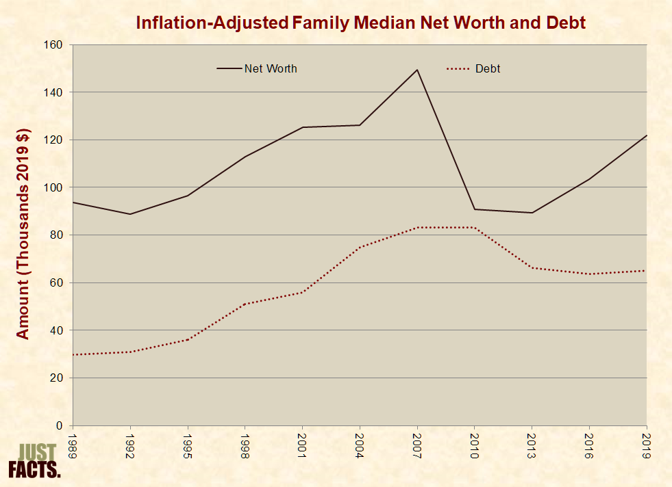
* Adjusted for inflation, median family debt peaked at $83,200 in 2010. Since 1989, inflation-adjusted median family net worth and debt have varied as follows:
* From 1989 to 2013, the inflation-adjusted average indebtedness of families in debt increased by 256%.[858]
* From 1989 to 2019, the portion of debt payments for the purchase of a primary residence rose from 71% to 78%. The portion of debt payments for other purchases varied as follows:
* In 2012, the 90+ day delinquency rate for student loans exceeded that of credit cards for the first time since reliable data on this measure became available in 2003.[861] It remained the most common type of delinquent debt until early 2020 when the federal government passed a law that suspended student loan payments in the wake of the Covid-19 pandemic through September 2020.[862] After this, President Trump and President Biden unilaterally extended this policy:[863]

* For more facts about student loans, visit Just Facts’ research on education.
* Per the Administrative Office of the U.S. Courts:
* Per the Federal Trade Commission:
* In 2005, Congress passed and President Bush signed the Bankruptcy Abuse Prevention and Consumer Protection Act of 2005.[869] The purpose of the bill was to:
* Congress passed this law in response “to many of the factors contributing to the increase in consumer bankruptcy filings,” such as the:
* The law mandated “the implementation and monitoring of”:
* During the Covid-19 pandemic the federal government and banks took actions to prevent bankruptcies.[873] [874]
* Since 2001 personal bankruptcy filings have varied as follows:

* At the close of 2022, the official debt of the United States government was $31.4 trillion ($31,419,689,421,558).[880] This amounted to:
* For comprehensive facts about the national debt, visit Just Facts’ research on this issue.
[1] Article: “Income Tax, Personal.” By David N. Hyman. Encyclopedia of Contemporary American Social Issues, Volume 1: Business and Economy. Edited by Michael Shally-Jensen. ABC-CLIO, 2011. Pages 170–178.
Pages 170–172:
What Is Income?
Income is a flow of purchasing power from earnings of labor, capital, land and other sources that a person receives over a period of one year. The most comprehensive definition of income views it as an annual acquisition of rights to command resources. Income can be used to consume goods and services during the year it is received, or it can be stored up for future use in subsequent years. Income stored up for future use is saving, which increases a person’s net worth (a measure of the value of assets less debts). The most comprehensive measure of income views it as the sum of annual consumption plus savings, where savings is any increase in net worth that can result from not spending earnings and other forms of income or from increases in the market value of such assets as stocks, bonds, or housing that a person might own. The annual increase in the value of a person’s existing assets are capital gains, which can either be realized (converted to cash) by selling an asset or unrealized (not turned into cash in the current year).
[2] Report: “American Housing Survey for the United States: 2015 – Appendix A. Subject Definitions and Table Index.” U.S. Department of Housing and Urban Development and U.S. Census Bureau. Last revised March 7, 2019. <www2.census.gov>
Appendix A–16:
“Money income” is the income received on a regular basis (exclusive of certain money receipts such as capital gains and lump-sum payments) before payments for personal income taxes, social security, union dues, Medicare deductions, etc. It includes income received from wages, salary, commissions, bonuses, and tips; self-employment income from own nonfarm or farm businesses, including proprietorships and partnerships; interest, dividends, net rental income, royalty income, or income from estates and trusts; Social Security or Railroad Retirement income; Supplemental Security Income (SSI); any cash public assistance or welfare payments from the state or local welfare office; retirement, survivor, or disability benefits; and any other sources of income received regularly such as Veterans’ (VA) payments, unemployment and/or worker’s compensation, child support, and alimony.
[3] Book: OECD Framework for Statistics on the Distribution of Household Income, Consumption and Wealth. Organization for Economic Cooperation and Development, 2013. <www.keepeek.com>
Pages 27–28: “Income allows people to satisfy their needs and pursue many other goals that they deem important to their lives, while wealth makes it possible to sustain these choices over time. Both income and wealth enhance individuals’ freedom to choose the lives that they want to live.”
[4] Report: “The Distribution of Household Income and Federal Taxes, 2013.” Congressional Budget Office, June 2016. <www.cbo.gov>
Page 2:
In 2013, according to the Congressional Budget Office’s estimates, average household market income—a comprehensive income measure that consists of labor income, business income, capital income (including capital gains), and retirement income—was approximately $86,000. Government transfers, which include benefits from programs such as Social Security, Medicare, and unemployment insurance, averaged approximately $14,000 per household. The sum of those two amounts, which equals before-tax income, was about $100,000, on average. In this report, CBO [Congressional Budget Office] analyzed the distribution of four types of federal taxes: individual income taxes, payroll (or social insurance) taxes, corporate income taxes, and excise taxes. Taken together, those taxes amounted to about $20,000 per household, on average, in 2013.1 Thus, average after-tax income—which equals market income plus government transfers minus federal taxes—was about $80,000, and the average federal tax rate (federal taxes divided by before-tax income) was about 20 percent.
1 Data for 2013 are the most recent available with complete information about tax payments. For more details, see the appendix.
[5] Webpage: “Income.” U.S. Census Bureau. Accessed January 4, 2023 at <www.census.gov>
“The Census Bureau reports income from several major household surveys and programs. Each differs from the others in some way, such as the length and detail of its questionnaire, the number of households included (sample size), and the methodology used.”
[6] Webpage: “Wages Earning & Benefits.” U.S. Department of Labor, Bureau of Labor Statistics. Accessed April 20, 2019 at <www.dol.gov>
Overview of BLS Statistics on Pay and Benefits
The Bureau of Labor Statistics (BLS) publishes a large amount of information on the wages, earnings, and benefits of workers. Generally, this information is categorized in one or more of the following ways:
• Geographic area (national regional, state, metropolitan area, or county data)
• Occupation (such as teacher); and
• Industry (such as manufacturing)
Additional categories, such as age, sex, or union membership, may be used in some cases.
[7] Webpage: “National Economic Accounts.” U.S. Department of Commerce, Bureau of Economic Analysis. Page last modified August 8, 2018. <www.bea.gov>
What are the National Economic Accounts?
BEA’s [Bureau of Economic Analysis’s] national economic statistics provide a comprehensive view of U.S. production, consumption, investment, exports and imports, and income and saving. These statistics are best known by summary measures such as gross domestic product (GDP), corporate profits, personal income and spending, and personal saving. …
• Disposable Personal Income
The income that’s left after people pay their taxes …
• Personal Income
Wages, Social Security, interest, rents, and other income received by U.S. residents
• Personal Saving Rate
The percentage of people’s disposable income that they save instead of spending
[8] Webpage: “SOI [Statistics of Income] Tax Stats – Individual Income Tax Return (Form 1040) Statistics.” Internal Revenue Service. Last updated December 14, 2018. <www.irs.gov>
Form 1040 Data
Publications
• Individual Income Tax Returns Publication (Complete Report) …
General Statistical Tables
• by Size of Adjusted Gross Income
• by Filing Status
• by Tax Rate and Income Percentile
• Time Series Data
[9] Webpage: “Survey of Consumer Finances: About.” Board of Governors of the Federal Reserve System. Last updated March 16, 2017. <www.federalreserve.gov>
The Survey of Consumer Finances (SCF) is normally a triennial cross-sectional survey of U.S. families. The survey data include information on families’ balance sheets, pensions, income, and demographic characteristics. Information is also included from related surveys of pension providers and the earlier such surveys conducted by the Federal Reserve Board. No other study for the country collects comparable information. Data from the SCF are widely used, from analysis at the Federal Reserve and other branches of government to scholarly work at the major economic research centers.
The survey has contained a panel element over two periods. Respondents to the 1983 survey were re-interviewed in 1986 and 1989. Respondents to the 2007 survey were re-interviewed in 2009.
The study is sponsored by the Federal Reserve Board in cooperation with the Department of the Treasury. Since 1992, data have been collected by the NORC at the University of Chicago.
To ensure the representativeness of the study, respondents are selected randomly using procedures described in the technical working papers on this web site. A strong attempt is made to select families from all economic strata.
Participation in the study is strictly voluntary. However, because only about 6,500 families were interviewed in the most recent study, every family selected is very important to the results. To maintain the scientific validity of the study, interviewers are not allowed to substitute respondents for families that do not participate. Thus, if a family declines to participate, it means that families like theirs may not be represented clearly in national discussions.
The confidentiality of the information provided in the study is of the highest importance to NORC and the Federal Reserve. Strenuous efforts are made to protect the privacy of participants, and in the history of the survey, there has never been a leak. The names of the participants in the survey are known only to NORC, which has more than 50 years of successful experience in collecting confidential information.
For the 1983 and 1989 surveys, a separate Survey of Pension Providers (SPP) was conducted to obtain detailed technical information on the pensions of SCF participants; data and documentation for the SPP appear under a separate link.
A link is also given for data and documentation from the 1962 Survey of Financial Characteristics of Consumers (SFCC) and the 1963 Survey of Changes in Family Finances (SCFF); these surveys are the most direct precursors of the SCF.
[10] Paper: “Integration of Micro and Macro Data on Consumer Income and Expenditures.” By Clinton P. McCully. U.S. Bureau of Economic Analysis, October 23, 2012. <www.justfacts.com>
Page 1:
Data on personal income and expenditures from the National Income and Product Accounts (NIPAs) produced by the Bureau of Economic Analysis (BEA) and from those based on household surveys have shown divergent trends in recent years. From 2000 to 2010, BEA estimates of real per capita disposable personal income (DPI) increased by 12 percent, while the Census Bureau’s Current Population Survey Statistical and Economic Supplement (CPS–ASEC) estimates of real median household money income decreased by 7 percent. Consumer expenditure data have shown similar differences between the BEA estimates and those based on the Bureau of Labor Statistics’ (BLS) Consumer Expenditure Survey (CE) program.
[11] Working paper: “A Comparison of Income Concepts: IRS Statistics of Income, Census Current Population Survey, and BLS [Bureau of Labor Statistics] Consumer Expenditure Survey.” By Eric L. Henry and Charles D. Day. Internal Revenue Service, 2005. <www.irs.gov>
Page 149:
Several Federal Government agencies produce statistics on individual and household income. Because of the differing purposes to which their data will be put, agencies use different definitions for income (income concepts), as well as different reporting units, sample designs, collection modes, and processing rules. Data users are faced with an array of choices, often without much help to sort out which data series best meets their needs or much guidance to reconcile results based on different sources of data.
[12] Webpage: “Income: About.” U.S. Census Bureau. Accessed October 27, 2020 at <bit.ly>
Census money income is defined as income received on a regular basis (exclusive of certain money receipts such as capital gains) before payments for personal income taxes, social security, union dues, medicare deductions, etc. Therefore, money income does not reflect the fact that some families receive part of their income in the form of noncash benefits, such as food stamps, health benefits, subsidized housing, and goods produced and consumed on the farm. In addition, money income does not reflect the fact that noncash benefits are also received by some nonfarm residents which may take the form of the use of business transportation and facilities, full or partial payments by business for retirement programs, medical and educational expenses, etc.
Data users should consider these elements when comparing income levels. Moreover, users should be aware that for many different reasons there is a tendency in household surveys for respondents to underreport their income. Based on an analysis of independently derived income estimates, the Census Bureau determined that respondents report income earned from wages or salaries much better than other sources of income and that the reported wage and salary income is nearly equal to independent estimates of aggregate income.
The Census Bureau also derives alternative income measures that systematically remove or add various income components such as deducting payroll taxes and federal and state income taxes and including the value of specific noncash benefits, food stamps, school lunches, housing subsidies, health insurance programs, and return on home equity.
[13] Paper: “Alternative Measures of Household Income: Personal Income, CPS Money Income, and Beyond.” By John Ruser, Adrienne Pilot, and Charles Nelson. U.S. Bureau of Economic Analysis, November 2004. <apps.bea.gov>
Pages 1–2:
Two of the most widely used measures of household income are BEA’s [Bureau of Economic Analysis’s] personal income and the Census Bureau’s money income. These two statistics spring from different traditions of measurement—personal income from national income accounting and money income from income distribution analysis. …
• The Current Population Survey (CPS) Annual Social and Economic Supplement is the source of the Census Bureau’s official national estimates of poverty. CPS money income is defined as total pre-tax cash income earned by persons, excluding certain lump sum payments and excluding capital gains.
• BEA estimates that personal income for the US was $8.678 trillion in 2001, as compared to a CPS money income estimate of $6.446 trillion.2 Over 64 percent of this $2.232 trillion gap—$1.429 trillion—can be accounted for by differences in the income types that are included in the two measures, including the $982 billion of property income that is counted in personal income but not in CPS money income.
• Half of the remaining $804 billion money income gap can be accounted for by BEA adjustments to proprietors’ income and wages and salaries for underreporting in BEA source data.
[14] Paper: “Alternative Measures of Household Income: BEA Personal Income, CPS Money Income, and Beyond.” By John Ruser, Adrienne Pilot, and Charles Nelson. U.S. Department of Commerce, Bureau of Economic Analysis, November 2004. <apps.bea.gov>
Page 2:
The Census Bureau has developed a number of alternative measures of money income that may measure economic well-being better than CPS [Current Population Survey] money income. These measures remove taxes, add in-kind transfers, add realized capital gains or losses, and add the imputed return on equity in own home. The Census Bureau has found that a broadened definition of income results in a more equal distribution of income and tends to reduce the gaps between the incomes of traditionally high- and low-income groups.
Page 4:
BEA Personal Income and Census Money Income
Two of the most widely used measures of household income are BEA’s [Bureau of Economic Analysis’s] personal income and the Census Bureau’s money income. These two measures differ in the scope of individuals covered, in the income items included, in the sources of the data and in the extent of disaggregation of the estimates. This section will discuss the general definitions, sources and uses of these two measures, while the next section presents a reconciliation of aggregate income estimates as a means of indicating the nature and size of differences.3
3A third widely used measure of income is IRS adjusted gross income (AGI). For a comparison of BEA personal income and IRS AGI, see Ledbetter (2004).
Pages 10–11:
Alternative Census Bureau Income Definitions
Description
The traditional money income concept is limited and does not provide a completely satisfactory measure of economic well-being. For example, money income (unlike BEA’s disposable income concept) does not include the effects of taxes and, therefore, does not reflect the effect of tax law changes on economic well-being. Similarly, the official measure of money income excludes the effect of noncash benefits (such as employment-related group health insurance and food stamps), which enhance economic well-being and are also included in BEA’s personal income. The Census Bureau has a fairly long history of producing estimates that address these shortcomings.
Since the early 1980s, the Census Bureau has published analysis showing the effect of using a broadened income definition on measures of economic well-being. Currently, annual Census Bureau reports on income and poverty show the effect of using an income measure that includes the effect of noncash benefits and taxes on the distribution of income, prevalence of poverty, and level of income inequality based on the 17 income definitions as summarized below:
• Definition 1: official money income
• Definition 1b: definition 1 plus capital gains/losses less taxes
• Definition 2: definition 1 less government cash transfers
• Definition 3: definition 2 plus capital gains/less capital losses
• Definition 4: definition 3 plus the value of employment-related health benefits
• Definition 5: definition 4 less Social Security payroll taxes
• Definition 6: definition 5 less federal income taxes (excluding the Earned • Income Tax Credit)
• Definition 7: definition 6 plus the Earned Income Tax Credit
• Definition 8: definition 7 less state income taxes
• Definition 9: definition 8 plus non-means-tested government cash transfers
• Definition 10: definition 9 plus the value of Medicare
• Definition 11: definition 10 plus the value of regular-price school lunches
• Definition 12: definition 11 plus means-tested cash transfers
• Definition 13: definition 12 plus the value of Medicaid
• Definition 14a: definition 13 plus the value of other means-tested government noncash transfers less Medicare and Medicaid
• Definition 14: definition 13 plus the value of other means-tested government noncash transfers
• Definition 15: definition 14 plus net imputed return on equity in own home
Obviously, the construction of 17 definitions of income was not based on the premise that each of these definitions represented a viable income concept. Rather, the construction of so many income definitions was to facilitate the analysis that examines which components of a broadened income measure are most responsible for the significant changes in income summary measures as one transitions from the money income concept to an expanded definition of well-being. That said, there are several expanded income definitions that the Census Bureau has found useful to track trends and differences between groups. For example, the 2002 CPS income report (U.S. Bureau of the Census, 2003) highlighted four definitions of income in addition to the traditional money income definition. These were definitions 1b, 14a, 14, and 15. It should be noted that in the 2002 income report for the first time these alternative income measures were featured in the main body of the report and presented along with the money income measures (in previous reports these figures were examined in supplemental report sections).
[15] Webpage: “Comparability of Current Population Survey Income Data with Other Data.” U.S. Census Bureau. Accessed January 13, 2017 at <www.census.gov>
The concepts used in the SIPP [Survey of Income and Program Participation] and the March supplement to the Current Population Survey (CPS) differ in some regards. These differences occur primarily between components of the income definition used in each survey and the manner in which certain reference units are categorized. An explanation of these differences follows.
Two basic units of reference common to both the SIPP and CPS are people and households. Groups of people living together, when combined based on relationship, form family units. A family refers to a group of two or more people related by birth, marriage, or adoption who reside together (one of whom is the householder). Two or more people who live together and are related to one another, but not related to the householder, form an unrelated subfamily. People in unrelated subfamilies are not included in the count of family members in the CPS, but are included as family members for the SIPP.
A unique feature of a longitudinal survey, such as SIPP, is its ability to capture change over time. A cross-sectional survey, such as CPS, does not have this feature and can only provide a series of snapshots of the socio-economic conditions that exist at different fixed points in time. CPS data are based on the demographic characteristics as they existed at the time the survey was conducted and are applied to the economic characteristics that existed for the previous calendar year. The demographic data in the SIPP are collected with the economic data throughout the calendar year and are likely to have changed during the year. In order to incorporate the effect of changes over time in family compositions in measures of SIPP income data, the data are presented for people rather than families. People are characterized by the income of their respective family unit based on living arrangements each month during the calendar year.
The definition of income used in the SIPP is basically the same as in the CPS. It reflects money income before taxes and does not include the value of noncash benefits such as employer-provided health insurance, food stamps, or Medicaid. Differences do exist however, they are:
• Accrued interest on Individual Retirement Accounts (IRA’s) KEOGH retirement plans, 401(k), and U.S. savings bonds; and educational assistance are excluded in SIPP and counted in the CPS.
• Lump-sum or one-time payments such as inheritances, insurance settlements, and lump-sum payments from a pension or retirement plan are counted in the SIPP and excluded in the CPS.
• Self-employment income (both farm and nonfarm) is counted in the CPS as a net amount, gross receipts minus operating expenses. In the SIPP, self-employment income includes a regular salary and/or any other income from the business.
[16] Article: “Comparison of BEA Estimates of Personal Income and IRS Estimates of Adjusted Gross Income.” By Mark Ledbetter. U.S. Department of Commerce, Bureau of Economic Analysis, Survey of Current Business, November 2007. <apps.bea.gov>
Page 35:
The Bureau of Economic Analysis (BEA) annually publishes a comparison of BEA’s measure of personal income and the Internal Revenue Service (IRS) measure of adjusted gross income (AGI); both are widely used measures of household income. This comparison features the “AGI gap,” which is the difference between BEA-derived estimates of adjusted gross income and the IRS estimate of adjusted gross income.
Key Terms
Adjusted gross income (AGI), for Federal income tax purposes, includes all income that is received in the form of money, property, and services that is not explicitly exempt by law.
Personal income is the income received by individuals, nonprofit institutions serving households, private noninsured welfare funds, and private trust funds from all sources. It includes income that is taxed, that is partly taxed (such as social security benefit payments), and that is tax-exempt (such as tax-exempt interest, nontaxable The AGI gap for each type of income is the difference transfer payments, and Medicare, Medicaid, and welfare benefit payments). It is the sum of “compensation of employees (received),” proprietors’ income, rental income, personal income receipts on assets, and personal current transfer receipts; contributions for government social insurance is subtracted. Personal income includes imputed income, but it excludes net gains from the sale of assets (capital gains), pension benefit payments, and employee and self-employed contributions for government social insurance. …
BEA-derived adjusted gross income is BEA’s conceptual measure of adjusted gross income without taxpayer misreporting. It is based on IRS tabulations of data from individual income tax returns, corporate income tax returns, nonfarm sole proprietorship income tax returns, partnership income tax returns, and extrapolated estimates for tax-exempt income and for private foundation income.
The AGI gap is the difference between the BEA-derived adjusted gross income and IRS adjusted gross income. The AGI gap for each type of income is the difference between the BEA-derived adjusted gross income for that type of income and the reallocated IRS adjusted gross income.
The relative AGI gap for each type of income shows the AGI gap by type of income as a percentage of the BEA-derived adjusted gross income by type of income.
Misreporting adjustments are adjustments to IRS source data that are designed to correct for the effects of taxpayer misreporting in the tax return tabulations and economic census data used in the NIPAs [National Income and Product Accounts]. These adjustments account for income that is underreported on tax returns and for the income that is earned by individuals who do not file tax returns.
[17] Webpage: “Frequently Asked Questions Related to the Poverty Guidelines and Poverty.” U.S. Department of Health and Human Services. Accessed March 4, 2023 at <aspe.hhs.gov>
Are the Poverty Guidelines Before-Tax or After-Tax? Are They Gross Income or Net Income? What Definition of Income Is Used with the Poverty Guidelines?
There is no simple answer to these questions. When determining program eligibility, some agencies compare before-tax income to the poverty guidelines, while other agencies compare after-tax income. Likewise, eligibility can be dependent on gross income, net income, or some other measure of income. Federal, state, and local program offices that use the poverty guidelines for eligibility purposes may define income in different ways. To find out the specific definition of income (before-tax, after-tax, etc.) used by a particular program or activity, one must consult the office or organization that administers that program.
While there is no standard definition of income for program eligibility purposes, the Census Bureau uses a standard definition of income for computing poverty statistics based on the official poverty thresholds. More information is available on the Census Bureau’s web site.
[18] Paper: “Alternative Measures of Household Income: Personal Income, CPS Money Income, and Beyond.” By John Ruser, Adrienne Pilot, and Charles Nelson. U.S. Bureau of Economic Analysis, November 2004. <apps.bea.gov>
Page 1: “Two of the most widely used measures of household income are BEA’s [Bureau of Economic Analysis’s] personal income and the Census Bureau’s money income.”
[19] Report: “Current Population Survey: 2022 Annual Social and Economic (ASEC) Supplement.” U.S. Census Bureau, November 30, 2022. <www2.census.gov>
Page G-1: “The CPS [Current Population Survey], sponsored jointly by the Census Bureau and the U.S. Bureau of Labor Statistics, is the country’s primary source of labor force statistics for the entire population. The Census Bureau and the U.S. Bureau of Labor Statistics also jointly sponsor the CPS ASEC [Annual Social and Economic Supplement].”
[20] Report: “Income in the United States: 2021.” By Jessica Semega and Melissa Kollar. U.S. Census Bureau, September 2022. <www.census.gov>
Page 55:
The Current Population Survey (CPS) is the longest-running survey conducted by the U.S. Census Bureau. The CPS is a household survey primarily used to collect employment data. The sample universe for the basic CPS consists of the resident civilian, noninstitutionalized population of the United States. …
The CPS Annual Social and Economic Supplement (CPS ASEC), which estimates in this report are based on, collects data in February, March, and April each year, asking detailed questions categorizing income into over 50 sources. The key purpose of the survey is to provide timely and comprehensive estimates of income, poverty, and health insurance and to measure change in these national-level estimates.
Page 15: “Table A-1. Income Summary Measures by Selected Characteristics: 2020 and 2021 … Type of Household … Race3 and Hispanic Origin of Householder … Age of Householder … Nativity of Householder … Region … Residence4 … Educational Attainment of Householder”
[21] Webpage: “Income: About.” U.S. Census Bureau. Accessed October 27, 2020 at <www.census.gov>
Census money income is defined as income received on a regular basis (exclusive of certain money receipts such as capital gains) before payments for personal income taxes, social security, union dues, medicare deductions, etc. Therefore, money income does not reflect the fact that some families receive part of their income in the form of noncash benefits, such as food stamps, health benefits, subsidized housing, and goods produced and consumed on the farm. In addition, money income does not reflect the fact that noncash benefits are also received by some nonfarm residents which may take the form of the use of business transportation and facilities, full or partial payments by business for retirement programs, medical and educational expenses, etc.
[22] Paper: “Integration of Micro and Macro Data on Consumer Income and Expenditures.” By Clinton P. McCully. U.S. Bureau of Economic Analysis, October 23, 2012. <www.justfacts.com>
Page 1 (of PDF): “The Current Population Survey Annual Statistical and Economic Supplement (CPS–ASEC) from the Census Bureau and the Consumer Expenditure Survey (CE) program from the Bureau of Labor Statistics (BLS) are household surveys used to produce micro estimates of household income and expenditures. “
Page 3:
Reports from businesses collected in economic censuses, sample surveys, and administratively are more reliable than household surveys, which for the CE Interview Survey and CPS–ASEC have issues with recalling income and expenditures and are subject to deliberate underreporting of certain items. For the CE Diary Survey, there are issues of what is sometimes called “diary fatigue”, which refers to the dropoff in recording of expenditures over time, evidenced by a persistent pattern of lower reported expenditures for the second of the one-week surveys compared to the first (CE 1983, 2003).
[23] Paper: “Household Surveys in Crisis.” By Bruce D. Meyer, Wallace K.C. Mok, and James X. Sullivan. The Journal of Economic Perspectives, Fall 2015. Pages 199–226. <www.jstor.org>
Page 199:
Large and nationally representative surveys are arguably among the most important innovations in social science research of the last century. … Household surveys are the source of official rates of unemployment, poverty, health insurance coverage, inflation, and other statistics that guide policy. They are also a primary source of data for economic research and are used to allocate government funds.
Page 200:
One productive approach to measuring the degree of bias in household surveys, along with addressing potential bias, is to compare survey results with administrative data. … We examine the quality of household survey data through comparisons with administrative data from nine large programs that receive considerable attention from both the research and policy community. For example, we compare the total dollar value of food stamp benefits reported, by all respondents in a survey to the total dollar value of food stamp benefits awarded as recorded in US Department of Agriculture, Food and Nutrition Service administrative data.
Our results show a sharp rise in the downward bias in household survey estimates of receipt rates and dollars received for most programs. In recent years, more than half of welfare dollars and nearly half of food stamp dollars have been missed in several major surveys. In particular, this measurement error typically takes the form of underreporting resulting from true program recipients being recorded as non-recipients. (Throughout this paper we use underreporting as a synonym for understatement or under-recording, since it is likely due to errors by both interviewers and interviewees.) We argue that although all three threats to survey quality are important, in the case of transfer program reporting and amounts, measurement error rather than unit nonresponse or item nonresponse appears to contribute the most bias.
Page 201:
The underreporting of transfer income in surveys has profound implication for our understanding of the low-income population and the effect of government programs for the poor. We point to evidence from linked administrative and survey data that indicates that this underreporting leads to an understatement of incomes at the bottom, the rate of program receipt, and the poverty-reducing effects of government programs—and thus to an overstatement of poverty and inequality.
[24] Report: “Income in the United States: 2021.” By Jessica Semega and Melissa Kollar. U.S. Census Bureau, September 2022. <www.census.gov>
Page 1: “This report presents estimates on income in the United States for calendar year 2021, based on information collected in the 2022 and earlier Current Population Survey Annual Social and Economic Supplements (CPS ASEC) conducted by the Census Bureau.*”
Page 13: “Moreover, readers should be aware that for many different reasons there is a tendency in household surveys for respondents to underreport their income.”
[25] Paper: “Income Measurement Error in Surveys: A Review.” By Jeffrey C. Moore, Linda L. Stinson, and Edward J. Welniak. U.S. Census Bureau, December 1997. <www.census.gov>
Page 2:
In its role as producer of the nation’s “official statistics,” the Census Bureau has, over the years, examined the quality of its income estimates through comparisons to independent estimates derived from independent, outside sources—e.g., the National Income and Products Accounts (NIPA), individual income tax data, Social Security Administration records, caseload statistics from agencies that administer various transfer programs, etc. Table 1, derived from Coder and Scoon-Rogers (1995), summarizes the results of recent work comparing survey-based estimates and independent benchmarks for an extensive set of income types. The Census Bureau’s two major income surveys, the Survey of Income and Program Participation (SIPP) and the Current Population Survey’s (CPS) March Income Supplement, supply the survey estimates. Two conclusions are immediately obvious from Table 1. First, a primary goal of SIPP was to provide more complete income data than CPS. The fact that SIPP’s estimates are generally closer to the benchmarks than CPS’s suggests that SIPP has had some success in meeting that goal—especially, perhaps, for transfer program income. Second, however, and even more pronounced, is the consistency with which the survey estimates fall short of the benchmarks—across surveys, across time, and across income categories.
[26] Report: “The Distribution of Household Income, 2020.” Congressional Budget Office, November 2023. <www.cbo.gov>
Page 2 (of PDF): “The Congressional Budget Office regularly analyzes household income in the United States. This report presents the distributions of household income, means-tested transfers, and federal taxes in 2020 and explores how they differ from the distributions in 2019.
Page 20:
Data
The core data used in CBO’s distributional analyses come from the Statistics of Income (SOI), a nationally representative sample of individual income tax returns collected by the IRS. That sample of tax returns becomes available to CBO approximately two years after the returns are filed. Data on household income are systematically and consistently reported in the SOI. The sample is therefore considered a reliable resource to use when analyzing the effects of fiscal policy on income. However, certain types of income are not reported in the SOI. In 2020, for example, the portion of payments from the Paycheck Protection Program that was not used to pay for employees’ wages was not taxable and therefore not available in the SOI data.
SOI data include information about tax filers’ family structure and age, but they do not include certain demographic information or data on people who do not file taxes. For that information, CBO uses data from the Annual Social and Economic Supplement of the Census Bureau’s Current Population Survey (CPS), which has data on the demographic characteristics and income of a large sample of households.6
CBO combines the two data sources, statistically matching each SOI record to a corresponding CPS record on the basis of demographic characteristics and income. Each pairing results in a new record that takes on some characteristics of the CPS record and some characteristics of the SOI record.7
Page 22:
Measures of Income, Federal Taxes, and Means-Tested Transfers
Most distributional analyses rely on a measure of annual income as the metric for ranking households. In CBO’s analyses of the distribution of household income, information about taxable income sources for tax-filing units that file individual income tax returns comes from the SOI, whereas information about nontaxable income sources and income for tax-filing units that do not file individual income tax returns comes from the CPS. Among households at the top of the income distribution, the majority of income data are drawn from the SOI. In contrast, among households in the lower and middle quintiles, a larger portion of income data is drawn from the CPS….
Pages 31–32:
Household income, unless otherwise indicated, refers to income before the effects of means-tested transfers and federal taxes are accounted for. Throughout this report, that income concept is called income before transfers and taxes. It consists of market income plus social insurance benefits.
Market income consists of the following five elements:
• Labor income. Wages and salaries, including those allocated by employees to 401(k) and other employment-based retirement plans; employer-paid health insurance premiums (as measured by the Census Bureau’s Current Population Survey); the employer’s share of payroll taxes for Social Security, Medicare, and federal unemployment insurance; and the share of corporate income taxes borne by workers.
• Business income. Net income from businesses and farms operated solely by their owners, partnership income, and income from S corporations.
• Capital gains. Net profits realized from the sale of assets (but not increases in the value of assets that have not been realized through sales).
• Capital income. Taxable and tax-exempt interest, dividends paid by corporations (but not dividends from S corporations, which are considered part of business income), rental income, and the share of corporate income taxes borne by capital owners.
• Other income sources. Income received in retirement for past services and other nongovernmental sources of income.
Social insurance benefits consist of benefits from Social Security (Old Age, Survivors, and Disability Insurance), Medicare (measured by the average cost to the government of providing those benefits), regular unemployment insurance (but not expanded unemployment compensation), and workers’ compensation.
Means-tested transfers are cash payments and in-kind services provided through federal, state, and local government assistance programs. Eligibility to receive such transfers is determined primarily on the basis of income, which must be below certain thresholds. Means-tested transfers are provided through the following programs: Medicaid and the Children’s Health Insurance Program (measured by the average cost to the federal government and state governments of providing those benefits); the Supplemental Nutrition Assistance Program (formerly known as the Food Stamp program); housing assistance programs; Supplemental Security Income; Temporary Assistance for Needy Families and its predecessor, Aid to Families With Dependent Children; child nutrition programs; the Low Income Home Energy Assistance Program; and state and local governments’ general assistance programs. For 2020, CBO included expanded unemployment compensation in means-tested transfers.
Average means-tested transfer rates are calculated as means-tested transfers (totaled within an income group) divided by income before transfers and taxes (totaled within an income group).
Federal taxes consist of individual income taxes, payroll (or social insurance) taxes, corporate income taxes, and excise taxes. Those four sources accounted for 94 percent of federal revenues in fiscal year 2020. Revenue sources not examined in this report include states’ deposits for unemployment insurance, estate and gift taxes, net income of the Federal Reserve System that is remitted to the Treasury, customs duties, and miscellaneous fees and fines.
In this analysis, taxes for a given year are the amount a household owes on the basis of income received in that year, regardless of when the taxes are paid. Those taxes comprise the following four categories:
• Individual income taxes. Individual income taxes are levied on income from all sources, except those excluded by law. Individual income taxes can be negative because they include the effects of refundable tax credits (including recovery rebate credits), which can result in net payments from the government. Specifically, if the amount of a refundable tax credit exceeds a filer’s tax liability before the credit is applied, the government pays that excess to the filer. Statutory marginal individual income tax rates are the rates set in law that apply to the last dollar of income.
• Payroll taxes. Payroll taxes are levied primarily on wages and salaries. They generally have a single rate and few exclusions, deductions, or credits. Payroll taxes include those that fund the Social Security trust funds, the Medicare trust fund, and unemployment insurance trust funds. The federal portion of the unemployment insurance payroll tax covers only administrative costs for the program; state-collected unemployment insurance payroll taxes are not included in the Congressional Budget Office’s measure of federal taxes (even though they are recorded as revenues in the federal budget). Households can be entitled to future social insurance benefits, including Social Security, Medicare, and unemployment insurance, as a result of paying payroll taxes. In this analysis, average payroll tax rates capture the taxes paid in a given year and do not capture the benefits that households may receive in the future.
• Corporate income taxes. Corporate income taxes are levied on the profits of U.S.–based corporations organized as C corporations. In this analysis, CBO allocated 75 percent of corporate income taxes in proportion to each household’s share of total capital income (including capital gains) and 25 percent to households in proportion to their share of labor income.
• Excise taxes. Sales of a wide variety of goods and services are subject to federal excise taxes. Most revenues from excise taxes are attributable to the sale of motor fuels (gasoline and diesel fuel), tobacco products, alcoholic beverages, and aviation-related goods and services (such as aviation fuel and airline tickets).
Average federal tax rates are calculated as federal taxes (totaled within an income group) divided by income before transfers and taxes (totaled within an income group).
Income after transfers and taxes is income before transfers and taxes plus means-tested transfers minus federal taxes.
Income groups are created by ranking households by their size-adjusted income before transfers and taxes. A household consists of people sharing a housing unit, regardless of their relationship. The income quintiles (or fifths of the distribution) contain approximately the same number of people but slightly different numbers of households…. Similarly, each full percentile (or hundredth of the distribution) contains approximately the same number of people but a different number of households. If a household has negative income (that is, if its business or investment losses exceed its other income), it is excluded from the lowest income group but included in totals.
NOTE: † See Just Facts’ research on the distribution of the federal tax burden for details about how the Congressional Budget Office determines the share of corporate income taxes borne by workers and owners of capital.
[27] Report: “The Distribution of Household Income and Federal Taxes, 2013.” Congressional Budget Office, June 2016. <www.cbo.gov>
Page 2:
In 2013, according to the Congressional Budget Office’s estimates, average household market income—a comprehensive income measure that consists of labor income, business income, capital income (including capital gains), and retirement income—was approximately $86,000. Government transfers, which include benefits from programs such as Social Security, Medicare, and unemployment insurance, averaged approximately $14,000 per household. The sum of those two amounts, which equals before-tax income, was about $100,000, on average. In this report, CBO [Congressional Budget Office] analyzed the distribution of four types of federal taxes: individual income taxes, payroll (or social insurance) taxes, corporate income taxes, and excise taxes. Taken together, those taxes amounted to about $20,000 per household, on average, in 2013.1 Thus, average after-tax income—which equals market income plus government transfers minus federal taxes—was about $80,000, and the average federal tax rate (federal taxes divided by before-tax income) was about 20 percent.
1 Data for 2013 are the most recent available with complete information about tax payments. For more details, see the appendix.
Pages 1–2:
Market income consists of labor income, business income, capital gains (profits realized from the sale of assets), capital income excluding capital gains, income received in retirement for past services, and other sources of income.
Government transfers are cash payments and in-kind benefits from social insurance and other government assistance programs. Those transfers include payments and benefits from federal, state, and local governments.
Before-tax income is market income plus government transfers. …
Income groups are created by ranking households by their size-adjusted income. A household consists of people sharing a housing unit, regardless of their relationships. Each income quintile (fifth) contains approximately equal numbers of people but different numbers of households. Similarly, each percentile (hundredth) contains approximately equal numbers of people but different numbers of households. If a household has negative income (that is, if its business or investment losses are larger than its other income), it is excluded from the lowest income group but included in totals.
Household income over time is adjusted for inflation using the price index for personal consumption expenditures as calculated by the Bureau of Economic Analysis.
[28] Paper: “Household Incomes in Tax Data: Using Addresses to Move from Tax Unit to Household Income Distributions.” By Jeff Larrimore, Jacob Mortenson, and David Splinter. Association for Public Policy Analysis and Management, October 2018. <appam.confex.com>
Page 1:
Over the past decade, research using administrative IRS tax return data has greatly expanded our understanding of incomes at the top of the U.S. income distribution (e.g., Piketty and Saez, 2003; Atkinson, Piketty, and Saez, 2011). However, researchers have been forced to adapt their analysis to fit the limitations of IRS tax return data. In particular, the absence of non-filers in tax return data has largely restricted analyses using tax records to the upper end of the income distribution. Additionally, tax returns provide information on those individuals appearing on the same tax return (a tax unit), but households may contain multiple tax units or non-filers. This situation has precluded household level analyses, which is the standard unit of analysis in both national and cross-national distributional studies.
Pages 2–3:
Standard tax return data exclude the nearly 15 percent of adults and 13 percent of household heads who do not file a tax return and are not claimed as dependents each year (Auten and Gee, 2009; Molloy, Smith, and Wozniak, 2011). These non-filers are not missing at random and are instead concentrated in the lower tail of the distribution—which means that researchers using tax return data observe only a truncated version of the income distribution. Most researchers partially overcome this problem by using tax return data only to analyze the top of the distribution and assuming that all non-filers have an income of 20 to 30 percent of average filer income (Piketty and Saez, 2003; Auten and Splinter, 2017). However, such an approach cannot be expanded to analyze lower-tail or distribution-wide inequality measures because it does not capture observation-level incomes for these non-filers.
[29] Webpage: “Income Measure Used for Distributional Analysis by the Tax Policy Center.” Tax Policy Center. Accessed January 5, 2023 at <www.taxpolicycenter.org>
The purpose of an income classifier is to proxy for taxpayers’ economic well-being and their ability to pay taxes. The measurement of income also matters importantly for the calculation and interpretation of effective tax rates (ETRs), the amount of taxes paid measured as a percentage of income. An income measure that understates economic income overstates effective tax rates and the burden of tax policy changes, measured either as the change in ETR or the percentage change in after-tax income. …
In the initial versions of the tax model, TPC [Tax Policy Center] used adjusted gross income (AGI) as the income classifier because it was readily available on income tax returns. But AGI has serious deficiencies. It is far from comprehensive—causing many households to be mischaracterized—and its definition can change with changes in tax law. It excludes such items as untaxed Social Security and pension benefits, tax-exempt employee benefits, income earned within retirement accounts, and tax-exempt interest.
[30] Report: “Tax Gap Estimates for Tax Years 2014–2016.” Internal Revenue Service, August 2022. <www.irs.gov>
Page 1:
The gross tax gap is the amount of true tax liability that is not paid voluntarily and timely. The estimated annual gross tax gap for Tax Years (TY) 2014–2016 is $496 billion. The voluntary compliance rate (VCR) is a ratio measure of relative compliance and is defined as the amount of “tax paid voluntarily and timely” divided by “total true tax”, expressed as a percentage. The estimated VCR is 85.0 percent.
The gross tax gap comprises three components:
• Nonfiling (tax not paid on time by those who do not file required returns on time, $39 billion),
• Underreporting (tax understated on timely filed returns, $398 billion), and
• Underpayment (tax that was reported on time, but not paid on time, $59 billion).
The net tax gap is the gross tax gap less tax that subsequently will be paid, either voluntarily but late or collected through IRS administrative and enforcement activities. The net tax gap is the portion of the gross tax gap that will not be paid. An estimated $68 billion of the gross tax gap eventually will be paid, resulting in a TY 2014–2016 net tax gap of $428 billion. The Net Compliance Rate (NCR) is defined as the sum of “tax paid voluntarily and timely” and “enforced and other late payments” divided by “total true tax”, expressed as a percentage. The estimated NCR is 87.0 percent.
The tax gap estimates are also segmented by type of tax. The individual income tax makes up the largest component of the tax gap, contributing $357 billion to the gross tax gap and $306 to the net tax gap. The second and third largest components involve employment tax, which includes self-employment, FICA and FUTA tax, and corporation income tax.
Page 6:
Tax gap concepts include several ratio measures expressed as rates or percentages. The purpose of these measures is to provide a relative measure of compliance or noncompliance. These measures are ratios of dollar amounts in the aggregate.2
The voluntary compliance rate (VCR) is defined as the amount of tax paid voluntarily and timely divided by total true tax, expressed as a percentage. The VCR is a complement to the gross tax gap.
The net compliance rate (NCR) is defined as the sum of all timely and enforced and other late payments divided by total true tax, expressed as a percentage. The NCR is a complement to the net tax gap. It is also equal to one minus the ratio of the net tax gap to total true tax.
Two other measures are used only for the underreporting tax gap. The net misreporting percentage (NMP) for a given line item is the NMA divided by the sum of the absolute values of the amounts that should have been reported. For most return or schedule line items, amounts that should have been reported can be positive only. However, amounts can be either positive or negative for business-related net income and certain other lines. So, for those line items where amounts can be negative, the denominator of the NMP is not the net of positive and negative amounts, but instead it is the total of all the amounts disregarding the sign in the calculation—that is, it is the sum of the absolute values. The NMP is a complement to the NMA.
The voluntary reporting rate, or VRR, is another underreporting tax gap measure. It is a measure of the overall extent of reporting compliance for a particular type of tax. It is defined as the amount of reported tax divided by the amount of tax that should have been reported. It reflects reporting compliance on timely filed returns and is a complement to the underreporting tax gap for a particular type of tax.
[31] Written statement: “How Tax Complexity Hinders Small Businesses: The Impact On Job Creation And Economic Growth.” By Nina E. Olson. Internal Revenue Service, National Taxpayer Advocate, April 13, 2011. <www.irs.gov>
Page 4:
IRS data show that when taxpayers have a choice about reporting their income, tax compliance rates are remarkably low. Workers who are classified as employees have little opportunity to underreport their earned income because it is subject to tax withholding. Employees thus report about 99 percent of their earned income. But among workers whose income is not subject to withholding, compliance rates plummet. IRS studies show that nonfarm sole proprietors report only 43 percent of their business income and unincorporated farming businesses report only 28 percent.
[32] Report: “Concepts and Methods of the U.S. National Income and Product Accounts (Chapter 5).” U.S. Bureau of Economic Analysis, December 2022. <www.bea.gov>
Pages 5-2–5-3:
PCE [personal consumption expenditures] measures the goods and services purchased by “persons”—that is, by households and by nonprofit institutions serving households (NPISHs)—who are resident in the United States. Persons resident in the United States are those who are physically located in the United States and who have resided, or expect to reside, in this country for 1 year or more. PCE also includes purchases by U.S. government civilian and military personnel stationed abroad, regardless of the duration of their assignments, and by U.S. residents who are traveling or working abroad for 1 year or less.3
Table 5.1 shows the kinds of transactions that are included in and excluded from PCE. Most of PCE consists of purchases of new goods and of services by households from private business. In addition, PCE includes purchases of new goods and of services by households from government and government enterprises, the costs incurred by NPISHs in providing services on behalf of households, net purchases of used goods by households, and purchases abroad of goods and services by U.S. residents traveling, working, or attending school in foreign countries. PCE also includes expenditures financed by third-party payers on behalf of households, such as employer-paid health insurance and medical care financed through government programs, and it includes expenses associated with life insurance and with private and government employee pension plans. Finally, PCE includes imputed purchases that keep PCE invariant to changes in the way that certain activities are carried out—for example, whether housing is rented or owned or whether employees are paid in cash or in kind. PCE transactions are valued in market prices, including sales and excise taxes.
In the NIPAs [national income and product accounts], final consumption expenditures by NPISHs is the portion of PCE that represents the services that are provided to households by NPISHs without explicit charge (such as the value of the education services provided by a nonprofit college or university that is over and above the tuition and other costs paid by or for the student’s household). It is equal to their gross output, which is measured as their current operating expenses (not including purchases of buildings and equipment, which are treated as private fixed investment), less their sales to households and to other sectors of the economy (such as sales of education services to employers) and less the value of any investment goods (such as software) that are produced directly by the NPISH. Services that are provided by NPISHs and are paid by or on behalf of households (such as the tuition and other costs) are already accounted for in PCE as purchases by households.
[33] Paper: “Integration of Micro and Macro Data on Consumer Income and Expenditures.” By Clinton P. McCully. U.S. Bureau of Economic Analysis, October 23, 2012. <www.justfacts.com>
Page 1 (of PDF):
This paper examines macro and micro sources of information about household income and expenditures. The Bureau of Economic Analysis (BEA) produces macro estimates of personal income and outlays (PI&O) that are part of the U.S. National Income and Product Accounts (NIPAs). … BEA’s estimates of personal income (PI), disposable personal income (DPI), personal outlays (PO), and personal consumption expenditures (PCE) cover the personal sector in the U.S. economy, consisting of resident households and of the nonprofit institutions serving households (NPISHs). … The integrated estimates are developed for the years 2006 through and 2010.
Pages 1–2:
Though the NIPA estimates of household income and expenditures are generally considered to be more accurate than estimates derived from the household surveys and are broader measures, they have no distributional information. A proposed solution, and the approach followed in this paper, is to reconcile the differences in these estimates through the integration of micro data from household surveys with national accounts data.1 This results in measures of income distribution and of other breakdowns of household income and consumption that are consistent with national accounts values and definitions. This is consistent with recommendations made in the “Report by the Commission on the Measurement of Economic Performance and Social Progress,” which stated that “distributional measures should be compatible in scope with average measures from the national accounts” (Stiglitz-Sen-Fitoussi, I.43).
1 BEA and its predecessor agency, the Office of Business Economics, periodically published estimates of the size distribution of national accounts personal income in the U.S. from the 1950s to the 1970s using CPS, Internal Revenue Service, and Federal Reserve Board data, and such estimates were published as part of the National Income and Product Accounts from 1959 to 1964. More recently, the Expert Group on Disparities in National Accounts, sponsored by the Organization for Economic Cooperation and Development (OECD) and Eurostat, has been working to develop internationally comparable estimates of the breakdown of household income and consumption on a national accounts basis, and Fixler and Johnson have done work to account for the distribution of income in the U.S. National Accounts.
[34] Report: “The Distribution of Household Income and Federal Taxes, 2013.” Congressional Budget Office, June 2016. <www.cbo.gov>
Page 2: “Household income over time is adjusted for inflation using the price index for personal consumption expenditures as calculated by the Bureau of Economic Analysis.”
[35] Webpage: “How the Census Bureau Measures Poverty.” U.S. Census Bureau. Accessed January 30, 2023 at <www.census.gov>
Following the Office of Management and Budget’s (OMB) Statistical Policy Directive 14, the Census Bureau uses a set of money income thresholds that vary by family size and composition to determine who is in poverty. If a family’s total income is less than the family’s threshold, then that family and every individual in it is considered in poverty. The official poverty thresholds do not vary geographically, but they are updated for inflation using the Consumer Price Index (CPI-U). The official poverty definition uses money income before taxes and does not include capital gains or noncash benefits (such as public housing, Medicaid, and food stamps).
[36] Webpage: “R-CPI-U-RS Homepage.” Consumer Price Index, U.S. Department of Labor, Bureau of Labor Statistics. Last modified March 12, 2021. <www.bls.gov>
The Bureau of Labor Statistics (BLS) has made numerous improvements to the Consumer Price Index (CPI) over the past several decades. While these improvements make the present and future CPI more accurate, historical price index series are not adjusted to reflect the improvements. Many researchers, however, expressed an interest in having a historical research series that was measured consistently over the entire period. Accordingly, the Consumer Price Index retroactive series using current methods (R-CPI-U-RS) presents an estimate of the CPI for all Urban Consumers (CPI-U) from 1978 to the present that incorporates, when possible, most of the improvements made over that time span into the entire series.
The primary users of the R-CPI-U-RS data are researchers that use it as a valuable proxy of a historical estimate of inflation using current methods. In addition, the Census Bureau currently makes use of the index to adjust some of its income measures for changes in the cost of living. The direct adjustment of individual CPI index series makes this the most detailed and systematic estimate available of a consistent CPI series. This measure attempts to answer the question, “What would have been the measured rate of inflation from 1978 forward had the methods currently used in calculating the CPI-U been in use since 1978?”
It is important to recognize that the R-CPI-U-RS provides an annual inflation series that adjusts for specific changes in BLS methodology. The R-CPI-U-RS is of use to forecasters and other researchers in analyzing the trends and other movements in consumer inflation over the last few decades. The measure should help answer the question of the degree to which the measured rate of inflation has been affected by some of the improvements BLS has made.
Limitations
The R-CPI-U-RS has some limitations. First, most estimates are based on BLS research covering a short period of time and extrapolated to a longer period. Therefore, there is uncertainty surrounding the magnitude of the adjustments. Second, there have been several improvements in the CPI not incorporated into the R-CPI-U-RS, either because they do not represent changes in methodology, because they had negligible impacts on the CPI’s growth rate, or because it was impossible to systematically estimate the impacts of the new methods in past years. Examples include changes in imputation methods, improvements in methods for pricing hospital services, and some changes in quality adjustment procedures, such as for wireless telephone services. A list of the changes incorporated in the R-CPI-U-RS is available in an online table.
Available data
The R-CPI-U-RS presents an estimate of the CPI for all Urban Consumers (CPI-U) from 1978 to the present that incorporates most of the improvements made over that time span into the entire series. Note that many of the improvements occurred prior to 2000 and the monthly percent change in the R-CPI-U-RS is very similar to the published CPI-U for years after 2001; many of the differences prior to 1999, however, are substantial, reflecting major methodological changes such as the switch to a rental equivalence approach for shelter in 1983 and the adoption of a geometric means formula in 1999. Monthly data are published once a year in March.
[37] Canberra Group Handbook on Household Income Statistics (2nd edition). United Nations Economic Commission for Europe, 2011. <www.unece.org>
Pages 2–3:
A household’s economic well-being can be expressed in terms of its access to goods and services. The more that a household can consume, the higher its level of economic wellbeing. …
Consumption is therefore an indicator of economic well-being. However, a household may be able to choose not to consume the maximum amount it could in any given period but to save at least some of the resources it has available. By saving, households can accumulate wealth through the purchase of assets which will generate income at a later date and serve as a “nest egg” for spending at a later time when income levels may be lower, or needs higher. As well as possibly earning a return for the household, ownership of wealth also affects their broader economic power and is another aspect of economic well-being. For example, households that own their own home outright generally have lower housing costs and may therefore have lower income requirements to satisfy their desired standard of living.
Thus to capture fully the extent of a household’s economic well-being it is desirable to look at a number of different aspects of their economic situation, including not only their income, but also their levels of wealth, changes in the value of that wealth and levels of consumption.
[38] Report: “The Distribution of Household Income and Federal Taxes, 2013.” Congressional Budget Office, June 2016. <www.cbo.gov>
Page 2: “Income groups are created by ranking households by their size-adjusted income. A household consists of people sharing a housing unit, regardless of their relationships.”
[39] Working paper: “Examining the Middle Class in the United States Using the Lens of the Supplemental Poverty Measure.” By Trudi Renwick and Kathleen Short. U.S. Census Bureau, September 30, 2014. <www.census.gov>
Pages 1–2:
II. Approaches to Defining the Middle Class
While much has been written on the middle class, there is no widely accepted approach to defining the middle class. Some analyses of the middle class equate being in the middle class with having income in the middle of the income distribution. Other analyses include in the middle class anyone who self-identifies as middle class. A third approach is to count as middle class anyone who has achieved certain aspirations—owning their own home, having savings for retirement and/or the ability to send their children to college. As may be expected, these disparate approaches do not identify the same people as being in the middle class.
Of the analyses that equate being in the middle class with having an income in the middle of the income distribution, many use median household income to “define” the middle class. This metric is a useful summary measure that can be tracked over time and across countries. Each year the Census Bureau publishes a number of tables providing estimates of median household income and median family income.
[40] Webpage: “Glossary.” U.S. Census Bureau. Accessed January 5, 2023 at <www.census.gov>
Median
This measure represents the middle value (if n is odd) or the average of the two middle values (if n is even) in an ordered list of data values. The median divides the total frequency distribution into two equal parts: one-half of the cases fall below the median and one-half of the cases exceed the median.
For example, the median income is the amount which divides the income distribution into two equal groups, one having incomes above the median, and the other having incomes below the median. The median for households, families, and unrelated individuals is based on all households, families, and unrelated individuals, respectively. The median for people is based on people with income.
[41] Report: “Was JFK Wrong? Does Rising Productivity No Longer Lead to Substantial Middle Class Gains?” By Stephen J. Rose. Information Technology & Innovation Foundation, December 16, 2014. <www2.itif.org>
Page 3:
So the phrase “stagnating income” does not apply to the experiences of real people but to “similarly-situated” people. This cumbersome phrase means that accurate comparisons involve comparing slots along the income ladder at different points in time. … There is always a group of families in the middle of the distribution; it is just not the same families. One should think of this comparison as the “group” comparison—i.e., comparing the median (or another wrung on the income ladder) over a specified number of years.
In other words, at any specific time, the economy is composed of people of varying ages and income. The people in the lowest rungs of the income ladder are often young people and older people with lots of assets, fewer expenses, and large government subsidies through Medicare, Social Security, and sometimes Medicaid. If we look 10, 20, or 30 years later, there has been a large changing of places (think of what happens on a crowded escalator with the same number of people at each level even though it is different people). Younger people are no longer on the bottom, but have moved up to a higher place on the income ladder; some old people have died and been replaced by people who were formerly in their prime-earning years; and new independent young people who were part of families now populate the lower rungs of the income ladder.
This means that comparing the income gains of the bottom three quintiles in 1979 and 2007 has little to do with the path of real families. Instead it is a commentary on the overall structure of the economy in that it compares low income people in 1979 to low income people in 2007 even though they aren’t the same people. … For example, the median income of those 20–31 in 1979 and married was $51,800 (2007 dollars), while 28 years later in 2007, the median of those 48 to 59 and married was $87,200.7
[42] Paper: “New Perspectives on Income Mobility and Inequality.” By Gerald Auten, Geoffrey Gee, and Nicholas Turner. National Tax Journal, December 2013. Pages 893–912. <www.law.upenn.edu>
Page 893:
This study examines several dimensions of income mobility and inequality—mobility of individuals through their peak earnings years, intergenerational mobility, and persistence in the top 1 percent. Its main findings can be summarized as follows. Half of those age 35–40 in the bottom quintile of their cohort moved to higher quintiles 20 years later; over 60 percent moved up relative to the full population. About 70 percent of dependents from low-income households were themselves in higher quintiles 20 years later. Younger generations gradually replaced those that dominated the top percentile in 1987. The results show the importance of life cycle effects and the changing composition of top income groups.
[43] Webpage: “Glossary of Statistical Terms: Purchasing Power Parities (PPPs).” Organization for Economic Co-operation and Development, September 25, 2001. Last updated 6/11/13. <bit.ly>
Definition:
Purchasing power parities (PPPs) are the rates of currency conversion that equalise the purchasing power of different currencies by eliminating the differences in price levels between countries. In their simplest form, PPPs are simply price relatives which show the ratio of the prices in national currencies of the same good or service in different countries.
Context:
PPPs are calculated in three stages:
– first for individual products,
– then for groups of products or basic headings and,
– finally, for groups of basic headings or aggregates.
The PPPs for basic headings are unweighted averages of the PPPs for individual products. The PPPs for aggregates are weighted averages of the PPPs for basic headings.
The weights used are the expenditures on the basic headings. PPPs at all stages are price relatives. They show how many units of currency A need to be spent in country A to obtain the same volume of a product or a basic heading or an aggregate that X units of currency B purchases in country B.
In the case of a single product, the “same volume” means “identical volume.” But in the case of the complex assortment of goods and services that make up an aggregate such as GDP [Gross Domestic Product], the “same volume” does not mean an “identical basket of goods and services.”
The composition of the basket will vary between countries according to their economic, social and cultural differences, but each basket will provide equivalent satisfaction or utility.
Also referred to as “parity” or “parities.”
[44] Report: “International Comparisons of GDP Per Capita and Per Hour, 1960–2011.” U.S. Department of Labor, Bureau of Labor Statistics, November 7, 2012. <www.bls.gov>
Page 1: “GDP per capita, when converted to U.S. dollars using purchasing power parities, is the most widely used income measure for international comparisons of living standards.”
Page 2:
Gross Domestic Product (GDP) is defined as the value of all market and some nonmarket goods and services produced within a country’s geographic borders. As such, it is the most comprehensive measure of a country’s economic output that is estimated by statistical agencies. GDP per capita may therefore be viewed as a rough indicator of a nation’s economic well being, while GDP per hour worked can provide a general picture of a country’s productivity.
[45] Report: “Eurostat–OECD Methodological Manual on Purchasing Power Parities.” Eurostat and the Organization for Economic Cooperation and Development, 2012. <www.oecd-ilibrary.org>
Pages 13–14:
In their simplest form, PPPs are nothing more than price relatives that show the ratio of the prices in national currencies of the same good or service in different countries. For example, if the price of a litre of Coca Cola is 2.30 euros in France and 2.00 dollars in the United States, then the
Page 14: PPP for Coca Cola between France and the United States is the ratio 2.30 euros to 2.00 dollars or 1.15 euros to the dollar. This means that for every dollar spent on Coca Cola in the United States, 1.15 euros would have to be spent in France to obtain the same quantity and quality—or, in other words, the same volume—of Coca Cola.
Page 15:
For example, if the PPP for GDP between the European Union and the United States is 1.28 dollars per euro and between the European Union and Japan it is 150 yen per euro, it can be inferred that a given volume of GDP that costs 1.00 euro in the European Union will cost 1.28 dollars in the United States and 150 yen in Japan. By converting these costs to a common currency with exchange rates (1 euro = 1.47 dollars = 151 yen), they can be compared. After conversion, the costs are 1.00 euro in the European Union, 0.87 euro in the United States and 0.99 euro in Japan from which it can be seen that the given volume of GDP costs more in the European Union and Japan than in United States and that it costs almost the same in the European Union and Japan. From this it can be concluded that the general price level of the European Union is higher than that of the United States but only marginally higher than that of Japan.
Page 16:
The purpose of the PPPs produced by Eurostat and the OECD is to make international price and volume comparisons of GDP and GDP expenditures. They are designed specifically to compare the size or the price levels of these expenditures between countries and should always be used to effect such comparisons. They are not designed, however, to make international comparisons of monetary flows, such as aid and foreign direct investment, or trade flows. For such comparisons, exchange rates should be used. Note that many international comparisons require neither PPPs nor exchange rates. For example, to compare real growth rates of GDP between countries, each country’s own published growth rate can be used. Similarly, for a comparison of government debt as a ratio of GDP, the ratios are calculated in each country’s own currency.
[46] Webpage: “Listings of WHO’s Response to Covid-19.” World Health Organization, June 29, 2020. Last updated January 29, 2021. <bit.ly>
“11 Mar 2020: Deeply concerned both by the alarming levels of spread and severity, and by the alarming levels of inaction, WHO made the assessment that Covid-19 could be characterized as a pandemic.”
[47] Calculated with the dataset: “The Distribution of Household Income, 2019.” Congressional Budget Office, November 2022. <www.cbo.gov>
“Table 3. Average Household Income, by Income Source and Income Group, 1979 to 2019, 2019 Dollars”
NOTES:
[48] Report: “The Distribution of Household Income, 2019.” Congressional Budget Office, November 2022. <www.cbo.gov>
Pages 33–34:
Data
The core data used in CBO’s [Congressional Budget Office’s] distributional analyses come from the Statistics of Income (SOI), a nationally representative sample of individual income tax returns collected by the Internal Revenue Service (IRS). The number of returns sampled grew over the period studied—1979 to 2019—rising from roughly 90,000 in some of the early years to more than 350,000 in later years. That sample of tax returns becomes available to CBO approximately two years after the returns are filed. …
Information from tax returns is supplemented with data from the Annual Social and Economic Supplement of the Census Bureau’s Current Population Survey (CPS), which contains survey data on the demographic characteristics and income of a large sample of households.5 The two sources are combined by statistically matching each SOI record to a corresponding CPS record on the basis of demographic characteristics and income. Each pairing results in a new record that takes on some characteristics of the CPS record and some characteristics of the SOI record.6
Page 35:
Measures of Income, Federal Taxes, and Means-Tested Transfers
Most distributional analyses rely on a measure of annual income as the metric for ranking households. In CBO’s analyses, information on taxable income sources for tax-filing units that file individual income tax returns comes from the SOI, whereas information on nontaxable income sources and income for tax-filing units that do not file individual income tax returns comes from the CPS. Among households at the top of the distribution, the majority of income data are drawn from the SOI. In contrast, among households in the lower and middle quintiles, a larger portion of income data is drawn from the CPS….
Pages 39–40:
Household income, unless otherwise indicated, refers to income before accounting for the effects of means-tested transfers and federal taxes. Throughout this report, that income concept is called income before transfers and taxes. It consists of market income plus social insurance benefits.
Market income consists of the following:
• Labor income. Wages and salaries, including those allocated by employees to 401(k) and other employment-based retirement plans; employer-paid health insurance premiums (as measured by the Census Bureau’s Current Population Survey); the employer’s share of Social Security, Medicare, and federal unemployment insurance payroll taxes; and the share of corporate income taxes borne by workers.
• Business income. Net income from businesses and farms operated solely by their owners, partnership income, and income from S corporations.
• Capital income (including capital gains). Net profits realized from the sale of assets (but not increases in the value of assets that have not been realized through sales); taxable and tax-exempt interest; dividends paid by corporations (but not dividends from S corporations, which are considered part of business income); positive rental income; and the share of corporate income taxes borne by capital owners.†
• Other income sources. Income received in retirement for past services and other nongovernmental sources of income.
Social insurance benefits consist of benefits from Social Security (Old Age, Survivors, and Disability Insurance), Medicare (measured by the average cost to the government of providing those benefits), unemployment insurance, and workers’ compensation.
Means-tested transfers are cash payments and in-kind services provided through federal, state, and local government assistance programs. Eligibility to receive such transfers is determined primarily on the basis of income, which must be below certain thresholds. Means-tested transfers are provided through the following programs: Medicaid and the Children’s Health Insurance Program (measured by the average cost to the government of providing those benefits); the Supplemental Nutrition Assistance Program (formerly known as the Food Stamp program); housing assistance programs; Supplemental Security Income; Temporary Assistance for Needy Families and its predecessor, Aid to Families With Dependent Children; child nutrition programs; the Low Income Home Energy Assistance Program; and state and local government general assistance programs.
Average means-tested transfer rates are calculated as means-tested transfers divided by income before transfers and taxes.
Federal taxes consist of individual income taxes, payroll (or social insurance) taxes, corporate income taxes, and excise taxes. Those four sources accounted for 93 percent of federal revenues in fiscal year 2019. Revenue sources not examined in this report include states’ deposits for unemployment insurance, estate and gift taxes, net income of the Federal Reserve System that is remitted to the Treasury, customs duties, and miscellaneous fees and fines.
In this analysis, taxes for a given year are the amount a household owes on the basis of income received that year, regardless of when the taxes are paid. Those taxes comprise the following:
• Individual income taxes. Individual income taxes are paid by U.S. citizens and residents on their income from all sources, except those sources exempted under the law. Individual income taxes can be negative because they include the effects of refundable tax credits, which can result in net payments from the government. Specifically, if the amount of a refundable tax credit exceeds a filer’s tax liability before the credit is applied, the government pays that excess to the filer. Statutory marginal individual income tax rates are the rates set in law that apply to the last dollar of income.
• Payroll taxes. Payroll taxes are levied primarily on wages and salaries and generally have a single rate and few exclusions, deductions, or credits. Payroll taxes include those that fund the Social Security trust funds, the Medicare trust fund, and unemployment insurance trust funds. The federal portion of the unemployment insurance payroll tax covers only administrative costs for the program; state-collected unemployment insurance payroll taxes are not included in the Congressional Budget Office’s measure of federal taxes (even though they are recorded as revenues in the federal budget). Households can be entitled to future social insurance benefits, including Social Security, Medicare, and unemployment insurance, as a result of paying payroll taxes. In this analysis, average payroll tax rates capture the taxes paid in a given year and do not capture the benefits households may receive in the future.
• Corporate income taxes. Corporate income taxes are levied on the profits of U.S.-based corporations organized as C corporations. In its analysis, CBO allocated 75 percent of corporate income taxes in proportion to each household’s share of total capital income (including capital gains) and 25 percent to households in proportion to their share of labor income.
• Excise taxes. Sales of a wide variety of goods and services are subject to federal excise taxes. Most revenues from excise taxes are attributable to the sale of motor fuels (gasoline and diesel fuel), tobacco products, alcoholic beverages, and aviation-related goods and services (such as aviation fuel and airline tickets).
Average federal tax rates are calculated as federal taxes divided by income before transfers and taxes.
Income after transfers and taxes is income before transfers and taxes plus means-tested transfers minus federal taxes.
Income groups are created by ranking households by their size-adjusted income before transfers and taxes. A household consists of people sharing a housing unit, regardless of their relationships. The income quintiles (fifths) contain approximately the same number of people but slightly different numbers of households…. Similarly, each full percentile (hundredth) contains approximately the same number of people but a different number of households. If a household has negative income (that is, if its business or investment losses are larger than its other income), it is excluded from the lowest income group but included in totals.
NOTE: † See Just Facts’ research on the distribution of the federal tax burden for details about how the Congressional Budget Office determines the share of corporate income taxes borne by workers and owners of capital.
[49] Article: “How Many Workers Are Employed in Sectors Directly Affected by Covid-19 Shutdowns, Where Do They Work, and How Much Do They Earn?” By Matthew Dey and Mark A. Loewenstein. U.S. Bureau of Labor Statistics Monthly Labor Review, April 2020. <www.bls.gov>
Page 1: “To reduce the spread of coronavirus disease 2019 (Covid-19), nearly all states have issued stay-at-home orders and shut down establishments deemed nonessential.”
[50] Article: “Covid-19 Restrictions.” USA Today. Last updated July 11, 2022. <www.usatoday.com>
Throughout the pandemic, officials across the United States have rolled out a patchwork of restrictions on social distancing, masking and other aspects of public life. The orders vary by state, county and even city. At the height of restrictions in late March and early April 2020, more than 310 million Americans were under directives ranging from “shelter in place” to “stay at home.” Restrictions are now ramping down in many places, as most states have fully reopened their economies.
[51] During 2020 and early 2021, federal politicians enacted six “Covid relief” laws that will cost a total of about $5.2 trillion over the course of a decade. This amounts to an average of $40,444 in spending per U.S. household.
Calculated with data from:
a) Report: “CBO Estimate for H.R. 6074, the Coronavirus Preparedness and Response Supplemental Appropriations Act, 2020, as Posted on March 4, 2020.” Congressional Budget Office, March 4, 2020. <www.cbo.gov>
b) Report: “Cost Estimate for H.R. 6201, Families First Coronavirus Response Act, Enacted as Public Law 116-127 on March 18, 2020.” Congressional Budget Office, April 2, 2020. <www.cbo.gov>
c) Report: “Cost Estimate for H.R. 748, CARES Act, Public Law 116-136.” Congressional Budget Office, April 16, 2020. <www.cbo.gov>
d) Report: “CBO Estimate for H.R. 266, the Paycheck Protection Program and Health Care Enhancement Act as Passed by the Senate on April 21, 2020.” Congressional Budget Office, April 22, 2020. <www.cbo.gov>
e) Report: “Estimate for Division N—Additional Coronavirus Response and Relief, H.R. 133, Consolidated Appropriations Act, 2021, Public Law 116-260, Enacted on December 27, 2020.” Congressional Budget Office, January 14, 2021. <www.cbo.gov>
f) Report: “Estimated Budgetary Effects of H.R. 1319, American Rescue Plan Act of 2021 as Passed by the Senate on March 6, 2021.” Congressional Budget Office, March 10, 2021. <www.cbo.gov>
g) Dataset: “HH-1. Households by Type: 1940 to Present.” U.S. Census Bureau, Current Population Survey, November 2021. <www.census.gov>
NOTE: An Excel file containing the data and calculations is available upon request.
[52] Calculated with the dataset: “The Distribution of Household Income, 2020.” Congressional Budget Office, November 2023. <www.cbo.gov>
“Table 3. Average Household Income, by Income Source and Income Group, 1979 to 2020, 2020 Dollars”
NOTES:
[53] Report: “The Distribution of Household Income, 2020.” Congressional Budget Office, November 2023. <www.cbo.gov>
Page 20:
Data
The core data used in CBO’s distributional analyses come from the Statistics of Income (SOI), a nationally representative sample of individual income tax returns collected by the IRS. That sample of tax returns becomes available to CBO approximately two years after the returns are filed. Data on household income are systematically and consistently reported in the SOI. The sample is therefore considered a reliable resource to use when analyzing the effects of fiscal policy on income. However, certain types of income are not reported in the SOI. In 2020, for example, the portion of payments from the Paycheck Protection Program that was not used to pay for employees’ wages was not taxable and therefore not available in the SOI data.
SOI data include information about tax filers’ family structure and age, but they do not include certain demographic information or data on people who do not file taxes. For that information, CBO uses data from the Annual Social and Economic Supplement of the Census Bureau’s Current Population Survey (CPS), which has data on the demographic characteristics and income of a large sample of households.6
CBO combines the two data sources, statistically matching each SOI record to a corresponding CPS record on the basis of demographic characteristics and income. Each pairing results in a new record that takes on some characteristics of the CPS record and some characteristics of the SOI record.7
Page 22:
Measures of Income, Federal Taxes, and Means-Tested Transfers
Most distributional analyses rely on a measure of annual income as the metric for ranking households. In CBO’s analyses of the distribution of household income, information about taxable income sources for tax-filing units that file individual income tax returns comes from the SOI, whereas information about nontaxable income sources and income for tax-filing units that do not file individual income tax returns comes from the CPS. Among households at the top of the income distribution, the majority of income data are drawn from the SOI. In contrast, among households in the lower and middle quintiles, a larger portion of income data is drawn from the CPS….
Pages 31–32:
Household income, unless otherwise indicated, refers to income before the effects of means-tested transfers and federal taxes are accounted for. Throughout this report, that income concept is called income before transfers and taxes. It consists of market income plus social insurance benefits.
Market income consists of the following five elements:
• Labor income. Wages and salaries, including those allocated by employees to 401(k) and other employment-based retirement plans; employer-paid health insurance premiums (as measured by the Census Bureau’s Current Population Survey); the employer’s share of payroll taxes for Social Security, Medicare, and federal unemployment insurance; and the share of corporate income taxes borne by workers.
• Business income. Net income from businesses and farms operated solely by their owners, partnership income, and income from S corporations.
• Capital gains. Net profits realized from the sale of assets (but not increases in the value of assets that have not been realized through sales).
• Capital income. Taxable and tax-exempt interest, dividends paid by corporations (but not dividends from S corporations, which are considered part of business income), rental income, and the share of corporate income taxes borne by capital owners.
• Other income sources. Income received in retirement for past services and other nongovernmental sources of income.
Social insurance benefits consist of benefits from Social Security (Old Age, Survivors, and Disability Insurance), Medicare (measured by the average cost to the government of providing those benefits), regular unemployment insurance (but not expanded unemployment compensation), and workers’ compensation.
Means-tested transfers are cash payments and in-kind services provided through federal, state, and local government assistance programs. Eligibility to receive such transfers is determined primarily on the basis of income, which must be below certain thresholds. Means-tested transfers are provided through the following programs: Medicaid and the Children’s Health Insurance Program (measured by the average cost to the federal government and state governments of providing those benefits); the Supplemental Nutrition Assistance Program (formerly known as the Food Stamp program); housing assistance programs; Supplemental Security Income; Temporary Assistance for Needy Families and its predecessor, Aid to Families With Dependent Children; child nutrition programs; the Low Income Home Energy Assistance Program; and state and local governments’ general assistance programs. For 2020, CBO included expanded unemployment compensation in means-tested transfers.
Average means-tested transfer rates are calculated as means-tested transfers (totaled within an income group) divided by income before transfers and taxes (totaled within an income group).
Federal taxes consist of individual income taxes, payroll (or social insurance) taxes, corporate income taxes, and excise taxes. Those four sources accounted for 94 percent of federal revenues in fiscal year 2020. Revenue sources not examined in this report include states’ deposits for unemployment insurance, estate and gift taxes, net income of the Federal Reserve System that is remitted to the Treasury, customs duties, and miscellaneous fees and fines.
In this analysis, taxes for a given year are the amount a household owes on the basis of income received in that year, regardless of when the taxes are paid. Those taxes comprise the following four categories:
• Individual income taxes. Individual income taxes are levied on income from all sources, except those excluded by law. Individual income taxes can be negative because they include the effects of refundable tax credits (including recovery rebate credits), which can result in net payments from the government. Specifically, if the amount of a refundable tax credit exceeds a filer’s tax liability before the credit is applied, the government pays that excess to the filer. Statutory marginal individual income tax rates are the rates set in law that apply to the last dollar of income.
• Payroll taxes. Payroll taxes are levied primarily on wages and salaries. They generally have a single rate and few exclusions, deductions, or credits. Payroll taxes include those that fund the Social Security trust funds, the Medicare trust fund, and unemployment insurance trust funds. The federal portion of the unemployment insurance payroll tax covers only administrative costs for the program; state-collected unemployment insurance payroll taxes are not included in the Congressional Budget Office’s measure of federal taxes (even though they are recorded as revenues in the federal budget). Households can be entitled to future social insurance benefits, including Social Security, Medicare, and unemployment insurance, as a result of paying payroll taxes. In this analysis, average payroll tax rates capture the taxes paid in a given year and do not capture the benefits that households may receive in the future.
• Corporate income taxes. Corporate income taxes are levied on the profits of U.S.–based corporations organized as C corporations. In this analysis, CBO allocated 75 percent of corporate income taxes in proportion to each household’s share of total capital income (including capital gains) and 25 percent to households in proportion to their share of labor income.
• Excise taxes. Sales of a wide variety of goods and services are subject to federal excise taxes. Most revenues from excise taxes are attributable to the sale of motor fuels (gasoline and diesel fuel), tobacco products, alcoholic beverages, and aviation-related goods and services (such as aviation fuel and airline tickets).
Average federal tax rates are calculated as federal taxes (totaled within an income group) divided by income before transfers and taxes (totaled within an income group).
Income after transfers and taxes is income before transfers and taxes plus means-tested transfers minus federal taxes.
Income groups are created by ranking households by their size-adjusted income before transfers and taxes. A household consists of people sharing a housing unit, regardless of their relationship. The income quintiles (or fifths of the distribution) contain approximately the same number of people but slightly different numbers of households…. Similarly, each full percentile (or hundredth of the distribution) contains approximately the same number of people but a different number of households. If a household has negative income (that is, if its business or investment losses exceed its other income), it is excluded from the lowest income group but included in totals.
NOTE: † See Just Facts’ research on the distribution of the federal tax burden for details about how the Congressional Budget Office determines the share of corporate income taxes borne by workers and owners of capital.
[54] Webpage: “Listings of WHO’s Response to Covid-19.” World Health Organization, June 29, 2020. Last updated January 29, 2021. <bit.ly>
“11 Mar 2020: Deeply concerned both by the alarming levels of spread and severity, and by the alarming levels of inaction, WHO made the assessment that Covid-19 could be characterized as a pandemic.”
[55] Calculated with the dataset: “The Distribution of Household Income, 2019.” Congressional Budget Office, November 2022. <www.cbo.gov>
“Table 3. Average Household Income, by Income Source and Income Group, 1979 to 2019, 2019 Dollars”
NOTES:
[56] Report: “The Distribution of Household Income, 2019.” Congressional Budget Office, November 2022. <www.cbo.gov>
Pages 33–34:
Data
The core data used in CBO’s [Congressional Budget Office’s] distributional analyses come from the Statistics of Income (SOI), a nationally representative sample of individual income tax returns collected by the Internal Revenue Service (IRS). The number of returns sampled grew over the period studied—1979 to 2019—rising from roughly 90,000 in some of the early years to more than 350,000 in later years. That sample of tax returns becomes available to CBO approximately two years after the returns are filed. …
Information from tax returns is supplemented with data from the Annual Social and Economic Supplement of the Census Bureau’s Current Population Survey (CPS), which contains survey data on the demographic characteristics and income of a large sample of households.5 The two sources are combined by statistically matching each SOI record to a corresponding CPS record on the basis of demographic characteristics and income. Each pairing results in a new record that takes on some characteristics of the CPS record and some characteristics of the SOI record.6
Page 35:
Measures of Income, Federal Taxes, and Means-Tested Transfers
Most distributional analyses rely on a measure of annual income as the metric for ranking households. In CBO’s analyses, information on taxable income sources for tax-filing units that file individual income tax returns comes from the SOI, whereas information on nontaxable income sources and income for tax-filing units that do not file individual income tax returns comes from the CPS. Among households at the top of the distribution, the majority of income data are drawn from the SOI. In contrast, among households in the lower and middle quintiles, a larger portion of income data is drawn from the CPS….
Pages 39–40:
Household income, unless otherwise indicated, refers to income before accounting for the effects of means-tested transfers and federal taxes. Throughout this report, that income concept is called income before transfers and taxes. It consists of market income plus social insurance benefits.
Market income consists of the following:
• Labor income. Wages and salaries, including those allocated by employees to 401(k) and other employment-based retirement plans; employer-paid health insurance premiums (as measured by the Census Bureau’s Current Population Survey); the employer’s share of Social Security, Medicare, and federal unemployment insurance payroll taxes; and the share of corporate income taxes borne by workers.
• Business income. Net income from businesses and farms operated solely by their owners, partnership income, and income from S corporations.
• Capital income (including capital gains). Net profits realized from the sale of assets (but not increases in the value of assets that have not been realized through sales); taxable and tax-exempt interest; dividends paid by corporations (but not dividends from S corporations, which are considered part of business income); positive rental income; and the share of corporate income taxes borne by capital owners.†
• Other income sources. Income received in retirement for past services and other nongovernmental sources of income.
Social insurance benefits consist of benefits from Social Security (Old Age, Survivors, and Disability Insurance), Medicare (measured by the average cost to the government of providing those benefits), unemployment insurance, and workers’ compensation.
Means-tested transfers are cash payments and in-kind services provided through federal, state, and local government assistance programs. Eligibility to receive such transfers is determined primarily on the basis of income, which must be below certain thresholds. Means-tested transfers are provided through the following programs: Medicaid and the Children’s Health Insurance Program (measured by the average cost to the government of providing those benefits); the Supplemental Nutrition Assistance Program (formerly known as the Food Stamp program); housing assistance programs; Supplemental Security Income; Temporary Assistance for Needy Families and its predecessor, Aid to Families With Dependent Children; child nutrition programs; the Low Income Home Energy Assistance Program; and state and local government general assistance programs.
Average means-tested transfer rates are calculated as means-tested transfers divided by income before transfers and taxes.
Federal taxes consist of individual income taxes, payroll (or social insurance) taxes, corporate income taxes, and excise taxes. Those four sources accounted for 93 percent of federal revenues in fiscal year 2019. Revenue sources not examined in this report include states’ deposits for unemployment insurance, estate and gift taxes, net income of the Federal Reserve System that is remitted to the Treasury, customs duties, and miscellaneous fees and fines.
In this analysis, taxes for a given year are the amount a household owes on the basis of income received that year, regardless of when the taxes are paid. Those taxes comprise the following:
• Individual income taxes. Individual income taxes are paid by U.S. citizens and residents on their income from all sources, except those sources exempted under the law. Individual income taxes can be negative because they include the effects of refundable tax credits, which can result in net payments from the government. Specifically, if the amount of a refundable tax credit exceeds a filer’s tax liability before the credit is applied, the government pays that excess to the filer. Statutory marginal individual income tax rates are the rates set in law that apply to the last dollar of income.
• Payroll taxes. Payroll taxes are levied primarily on wages and salaries and generally have a single rate and few exclusions, deductions, or credits. Payroll taxes include those that fund the Social Security trust funds, the Medicare trust fund, and unemployment insurance trust funds. The federal portion of the unemployment insurance payroll tax covers only administrative costs for the program; state-collected unemployment insurance payroll taxes are not included in the Congressional Budget Office’s measure of federal taxes (even though they are recorded as revenues in the federal budget). Households can be entitled to future social insurance benefits, including Social Security, Medicare, and unemployment insurance, as a result of paying payroll taxes. In this analysis, average payroll tax rates capture the taxes paid in a given year and do not capture the benefits households may receive in the future.
• Corporate income taxes. Corporate income taxes are levied on the profits of U.S.-based corporations organized as C corporations. In its analysis, CBO allocated 75 percent of corporate income taxes in proportion to each household’s share of total capital income (including capital gains) and 25 percent to households in proportion to their share of labor income.
• Excise taxes. Sales of a wide variety of goods and services are subject to federal excise taxes. Most revenues from excise taxes are attributable to the sale of motor fuels (gasoline and diesel fuel), tobacco products, alcoholic beverages, and aviation-related goods and services (such as aviation fuel and airline tickets).
Average federal tax rates are calculated as federal taxes divided by income before transfers and taxes.
Income after transfers and taxes is income before transfers and taxes plus means-tested transfers minus federal taxes.
Income groups are created by ranking households by their size-adjusted income before transfers and taxes. A household consists of people sharing a housing unit, regardless of their relationships. The income quintiles (fifths) contain approximately the same number of people but slightly different numbers of households…. Similarly, each full percentile (hundredth) contains approximately the same number of people but a different number of households. If a household has negative income (that is, if its business or investment losses are larger than its other income), it is excluded from the lowest income group but included in totals.
NOTE: † See Just Facts’ research on the distribution of the federal tax burden for details about how the Congressional Budget Office determines the share of corporate income taxes borne by workers and owners of capital.
[57] Article: “How Many Workers Are Employed in Sectors Directly Affected by Covid-19 Shutdowns, Where Do They Work, and How Much Do They Earn?” By Matthew Dey and Mark A. Loewenstein. U.S. Bureau of Labor Statistics Monthly Labor Review, April 2020. <www.bls.gov>
Page 1: “To reduce the spread of coronavirus disease 2019 (Covid-19), nearly all states have issued stay-at-home orders and shut down establishments deemed nonessential.”
[58] Article: “Covid-19 Restrictions.” USA Today. Last updated July 11, 2022. <www.usatoday.com>
Throughout the pandemic, officials across the United States have rolled out a patchwork of restrictions on social distancing, masking and other aspects of public life. The orders vary by state, county and even city. At the height of restrictions in late March and early April 2020, more than 310 million Americans were under directives ranging from “shelter in place” to “stay at home.” Restrictions are now ramping down in many places, as most states have fully reopened their economies.
[59] During 2020 and early 2021, federal politicians enacted six “Covid relief” laws that will cost a total of about $5.2 trillion over the course of a decade. This amounts to an average of $40,444 in spending per U.S. household.
Calculated with data from:
a) Report: “CBO Estimate for H.R. 6074, the Coronavirus Preparedness and Response Supplemental Appropriations Act, 2020, as Posted on March 4, 2020.” Congressional Budget Office, March 4, 2020. <www.cbo.gov>
b) Report: “Cost Estimate for H.R. 6201, Families First Coronavirus Response Act, Enacted as Public Law 116-127 on March 18, 2020.” Congressional Budget Office, April 2, 2020. <www.cbo.gov>
c) Report: “Cost Estimate for H.R. 748, CARES Act, Public Law 116-136.” Congressional Budget Office, April 16, 2020. <www.cbo.gov>
d) Report: “CBO Estimate for H.R. 266, the Paycheck Protection Program and Health Care Enhancement Act as Passed by the Senate on April 21, 2020.” Congressional Budget Office, April 22, 2020. <www.cbo.gov>
e) Report: “Estimate for Division N—Additional Coronavirus Response and Relief, H.R. 133, Consolidated Appropriations Act, 2021, Public Law 116-260, Enacted on December 27, 2020.” Congressional Budget Office, January 14, 2021. <www.cbo.gov>
f) Report: “Estimated Budgetary Effects of H.R. 1319, American Rescue Plan Act of 2021 as Passed by the Senate on March 6, 2021.” Congressional Budget Office, March 10, 2021. <www.cbo.gov>
g) Dataset: “HH-1. Households by Type: 1940 to Present.” U.S. Census Bureau, Current Population Survey, November 2021. <www.census.gov>
NOTE: An Excel file containing the data and calculations is available upon request.
[60] Calculated with the dataset: “The Distribution of Household Income, 2020.” Congressional Budget Office, November 2023. <www.cbo.gov>
“Table 3. Average Household Income, by Income Source and Income Group, 1979 to 2020, 2020 Dollars”
NOTES:
[61] Report: “The Distribution of Household Income, 2020.” Congressional Budget Office, November 2023. <www.cbo.gov>
Page 20:
Data
The core data used in CBO’s distributional analyses come from the Statistics of Income (SOI), a nationally representative sample of individual income tax returns collected by the IRS. That sample of tax returns becomes available to CBO approximately two years after the returns are filed. Data on household income are systematically and consistently reported in the SOI. The sample is therefore considered a reliable resource to use when analyzing the effects of fiscal policy on income. However, certain types of income are not reported in the SOI. In 2020, for example, the portion of payments from the Paycheck Protection Program that was not used to pay for employees’ wages was not taxable and therefore not available in the SOI data.
SOI data include information about tax filers’ family structure and age, but they do not include certain demographic information or data on people who do not file taxes. For that information, CBO uses data from the Annual Social and Economic Supplement of the Census Bureau’s Current Population Survey (CPS), which has data on the demographic characteristics and income of a large sample of households.6
CBO combines the two data sources, statistically matching each SOI record to a corresponding CPS record on the basis of demographic characteristics and income. Each pairing results in a new record that takes on some characteristics of the CPS record and some characteristics of the SOI record.7
Page 22:
Measures of Income, Federal Taxes, and Means-Tested Transfers
Most distributional analyses rely on a measure of annual income as the metric for ranking households. In CBO’s analyses of the distribution of household income, information about taxable income sources for tax-filing units that file individual income tax returns comes from the SOI, whereas information about nontaxable income sources and income for tax-filing units that do not file individual income tax returns comes from the CPS. Among households at the top of the income distribution, the majority of income data are drawn from the SOI. In contrast, among households in the lower and middle quintiles, a larger portion of income data is drawn from the CPS….
Pages 31–32:
Household income, unless otherwise indicated, refers to income before the effects of means-tested transfers and federal taxes are accounted for. Throughout this report, that income concept is called income before transfers and taxes. It consists of market income plus social insurance benefits.
Market income consists of the following five elements:
• Labor income. Wages and salaries, including those allocated by employees to 401(k) and other employment-based retirement plans; employer-paid health insurance premiums (as measured by the Census Bureau’s Current Population Survey); the employer’s share of payroll taxes for Social Security, Medicare, and federal unemployment insurance; and the share of corporate income taxes borne by workers.
• Business income. Net income from businesses and farms operated solely by their owners, partnership income, and income from S corporations.
• Capital gains. Net profits realized from the sale of assets (but not increases in the value of assets that have not been realized through sales).
• Capital income. Taxable and tax-exempt interest, dividends paid by corporations (but not dividends from S corporations, which are considered part of business income), rental income, and the share of corporate income taxes borne by capital owners.
• Other income sources. Income received in retirement for past services and other nongovernmental sources of income.
Social insurance benefits consist of benefits from Social Security (Old Age, Survivors, and Disability Insurance), Medicare (measured by the average cost to the government of providing those benefits), regular unemployment insurance (but not expanded unemployment compensation), and workers’ compensation.
Means-tested transfers are cash payments and in-kind services provided through federal, state, and local government assistance programs. Eligibility to receive such transfers is determined primarily on the basis of income, which must be below certain thresholds. Means-tested transfers are provided through the following programs: Medicaid and the Children’s Health Insurance Program (measured by the average cost to the federal government and state governments of providing those benefits); the Supplemental Nutrition Assistance Program (formerly known as the Food Stamp program); housing assistance programs; Supplemental Security Income; Temporary Assistance for Needy Families and its predecessor, Aid to Families With Dependent Children; child nutrition programs; the Low Income Home Energy Assistance Program; and state and local governments’ general assistance programs. For 2020, CBO included expanded unemployment compensation in means-tested transfers.
Average means-tested transfer rates are calculated as means-tested transfers (totaled within an income group) divided by income before transfers and taxes (totaled within an income group).
Federal taxes consist of individual income taxes, payroll (or social insurance) taxes, corporate income taxes, and excise taxes. Those four sources accounted for 94 percent of federal revenues in fiscal year 2020. Revenue sources not examined in this report include states’ deposits for unemployment insurance, estate and gift taxes, net income of the Federal Reserve System that is remitted to the Treasury, customs duties, and miscellaneous fees and fines.
In this analysis, taxes for a given year are the amount a household owes on the basis of income received in that year, regardless of when the taxes are paid. Those taxes comprise the following four categories:
• Individual income taxes. Individual income taxes are levied on income from all sources, except those excluded by law. Individual income taxes can be negative because they include the effects of refundable tax credits (including recovery rebate credits), which can result in net payments from the government. Specifically, if the amount of a refundable tax credit exceeds a filer’s tax liability before the credit is applied, the government pays that excess to the filer. Statutory marginal individual income tax rates are the rates set in law that apply to the last dollar of income.
• Payroll taxes. Payroll taxes are levied primarily on wages and salaries. They generally have a single rate and few exclusions, deductions, or credits. Payroll taxes include those that fund the Social Security trust funds, the Medicare trust fund, and unemployment insurance trust funds. The federal portion of the unemployment insurance payroll tax covers only administrative costs for the program; state-collected unemployment insurance payroll taxes are not included in the Congressional Budget Office’s measure of federal taxes (even though they are recorded as revenues in the federal budget). Households can be entitled to future social insurance benefits, including Social Security, Medicare, and unemployment insurance, as a result of paying payroll taxes. In this analysis, average payroll tax rates capture the taxes paid in a given year and do not capture the benefits that households may receive in the future.
• Corporate income taxes. Corporate income taxes are levied on the profits of U.S.–based corporations organized as C corporations. In this analysis, CBO allocated 75 percent of corporate income taxes in proportion to each household’s share of total capital income (including capital gains) and 25 percent to households in proportion to their share of labor income.
• Excise taxes. Sales of a wide variety of goods and services are subject to federal excise taxes. Most revenues from excise taxes are attributable to the sale of motor fuels (gasoline and diesel fuel), tobacco products, alcoholic beverages, and aviation-related goods and services (such as aviation fuel and airline tickets).
Average federal tax rates are calculated as federal taxes (totaled within an income group) divided by income before transfers and taxes (totaled within an income group).
Income after transfers and taxes is income before transfers and taxes plus means-tested transfers minus federal taxes.
Income groups are created by ranking households by their size-adjusted income before transfers and taxes. A household consists of people sharing a housing unit, regardless of their relationship. The income quintiles (or fifths of the distribution) contain approximately the same number of people but slightly different numbers of households…. Similarly, each full percentile (or hundredth of the distribution) contains approximately the same number of people but a different number of households. If a household has negative income (that is, if its business or investment losses exceed its other income), it is excluded from the lowest income group but included in totals.
NOTE: † See Just Facts’ research on the distribution of the federal tax burden for details about how the Congressional Budget Office determines the share of corporate income taxes borne by workers and owners of capital.
[62] Calculated with the dataset: “The Distribution of Household Income, 2020.” Congressional Budget Office, November 2023. <www.cbo.gov>
“Table 3. Average Household Income, by Income Source and Income Group, 1979 to 2020, 2020 Dollars”
NOTES:
[63] Report: “The Distribution of Household Income, 2020.” Congressional Budget Office, November 2023. <www.cbo.gov>
Page 20:
Data
The core data used in CBO’s distributional analyses come from the Statistics of Income (SOI), a nationally representative sample of individual income tax returns collected by the IRS. That sample of tax returns becomes available to CBO approximately two years after the returns are filed. Data on household income are systematically and consistently reported in the SOI. The sample is therefore considered a reliable resource to use when analyzing the effects of fiscal policy on income. However, certain types of income are not reported in the SOI. In 2020, for example, the portion of payments from the Paycheck Protection Program that was not used to pay for employees’ wages was not taxable and therefore not available in the SOI data.
SOI data include information about tax filers’ family structure and age, but they do not include certain demographic information or data on people who do not file taxes. For that information, CBO uses data from the Annual Social and Economic Supplement of the Census Bureau’s Current Population Survey (CPS), which has data on the demographic characteristics and income of a large sample of households.6
CBO combines the two data sources, statistically matching each SOI record to a corresponding CPS record on the basis of demographic characteristics and income. Each pairing results in a new record that takes on some characteristics of the CPS record and some characteristics of the SOI record.7
Page 22:
Measures of Income, Federal Taxes, and Means-Tested Transfers
Most distributional analyses rely on a measure of annual income as the metric for ranking households. In CBO’s analyses of the distribution of household income, information about taxable income sources for tax-filing units that file individual income tax returns comes from the SOI, whereas information about nontaxable income sources and income for tax-filing units that do not file individual income tax returns comes from the CPS. Among households at the top of the income distribution, the majority of income data are drawn from the SOI. In contrast, among households in the lower and middle quintiles, a larger portion of income data is drawn from the CPS….
Pages 31–32:
Household income, unless otherwise indicated, refers to income before the effects of means-tested transfers and federal taxes are accounted for. Throughout this report, that income concept is called income before transfers and taxes. It consists of market income plus social insurance benefits.
Market income consists of the following five elements:
• Labor income. Wages and salaries, including those allocated by employees to 401(k) and other employment-based retirement plans; employer-paid health insurance premiums (as measured by the Census Bureau’s Current Population Survey); the employer’s share of payroll taxes for Social Security, Medicare, and federal unemployment insurance; and the share of corporate income taxes borne by workers.
• Business income. Net income from businesses and farms operated solely by their owners, partnership income, and income from S corporations.
• Capital gains. Net profits realized from the sale of assets (but not increases in the value of assets that have not been realized through sales).
• Capital income. Taxable and tax-exempt interest, dividends paid by corporations (but not dividends from S corporations, which are considered part of business income), rental income, and the share of corporate income taxes borne by capital owners.
• Other income sources. Income received in retirement for past services and other nongovernmental sources of income.
Social insurance benefits consist of benefits from Social Security (Old Age, Survivors, and Disability Insurance), Medicare (measured by the average cost to the government of providing those benefits), regular unemployment insurance (but not expanded unemployment compensation), and workers’ compensation.
Means-tested transfers are cash payments and in-kind services provided through federal, state, and local government assistance programs. Eligibility to receive such transfers is determined primarily on the basis of income, which must be below certain thresholds. Means-tested transfers are provided through the following programs: Medicaid and the Children’s Health Insurance Program (measured by the average cost to the federal government and state governments of providing those benefits); the Supplemental Nutrition Assistance Program (formerly known as the Food Stamp program); housing assistance programs; Supplemental Security Income; Temporary Assistance for Needy Families and its predecessor, Aid to Families With Dependent Children; child nutrition programs; the Low Income Home Energy Assistance Program; and state and local governments’ general assistance programs. For 2020, CBO included expanded unemployment compensation in means-tested transfers.
Average means-tested transfer rates are calculated as means-tested transfers (totaled within an income group) divided by income before transfers and taxes (totaled within an income group).
Federal taxes consist of individual income taxes, payroll (or social insurance) taxes, corporate income taxes, and excise taxes. Those four sources accounted for 94 percent of federal revenues in fiscal year 2020. Revenue sources not examined in this report include states’ deposits for unemployment insurance, estate and gift taxes, net income of the Federal Reserve System that is remitted to the Treasury, customs duties, and miscellaneous fees and fines.
In this analysis, taxes for a given year are the amount a household owes on the basis of income received in that year, regardless of when the taxes are paid. Those taxes comprise the following four categories:
• Individual income taxes. Individual income taxes are levied on income from all sources, except those excluded by law. Individual income taxes can be negative because they include the effects of refundable tax credits (including recovery rebate credits), which can result in net payments from the government. Specifically, if the amount of a refundable tax credit exceeds a filer’s tax liability before the credit is applied, the government pays that excess to the filer. Statutory marginal individual income tax rates are the rates set in law that apply to the last dollar of income.
• Payroll taxes. Payroll taxes are levied primarily on wages and salaries. They generally have a single rate and few exclusions, deductions, or credits. Payroll taxes include those that fund the Social Security trust funds, the Medicare trust fund, and unemployment insurance trust funds. The federal portion of the unemployment insurance payroll tax covers only administrative costs for the program; state-collected unemployment insurance payroll taxes are not included in the Congressional Budget Office’s measure of federal taxes (even though they are recorded as revenues in the federal budget). Households can be entitled to future social insurance benefits, including Social Security, Medicare, and unemployment insurance, as a result of paying payroll taxes. In this analysis, average payroll tax rates capture the taxes paid in a given year and do not capture the benefits that households may receive in the future.
• Corporate income taxes. Corporate income taxes are levied on the profits of U.S.–based corporations organized as C corporations. In this analysis, CBO allocated 75 percent of corporate income taxes in proportion to each household’s share of total capital income (including capital gains) and 25 percent to households in proportion to their share of labor income.
• Excise taxes. Sales of a wide variety of goods and services are subject to federal excise taxes. Most revenues from excise taxes are attributable to the sale of motor fuels (gasoline and diesel fuel), tobacco products, alcoholic beverages, and aviation-related goods and services (such as aviation fuel and airline tickets).
Average federal tax rates are calculated as federal taxes (totaled within an income group) divided by income before transfers and taxes (totaled within an income group).
Income after transfers and taxes is income before transfers and taxes plus means-tested transfers minus federal taxes.
Income groups are created by ranking households by their size-adjusted income before transfers and taxes. A household consists of people sharing a housing unit, regardless of their relationship. The income quintiles (or fifths of the distribution) contain approximately the same number of people but slightly different numbers of households…. Similarly, each full percentile (or hundredth of the distribution) contains approximately the same number of people but a different number of households. If a household has negative income (that is, if its business or investment losses exceed its other income), it is excluded from the lowest income group but included in totals.
NOTE: † See Just Facts’ research on the distribution of the federal tax burden for details about how the Congressional Budget Office determines the share of corporate income taxes borne by workers and owners of capital.
[64] Economists typically use a “comprehensive measure of income” to calculate effective tax rates because this provides a complete “measure of ability to pay” taxes.† In keeping with this, Just Facts determines effective tax rates by dividing all measurable taxes by all income. The Congressional Budget Office (CBO) previously did the same,‡ but in 2018, CBO announced that it would exclude means-tested transfers from its measures of income and effective tax rates.§ #
Given this change, Just Facts now uses CBO data to determine comprehensive income and effective tax rates by adding back the means-tested transfers that CBO publishes but takes out of these measures. To do this, Just Facts makes a simplifying assumption that households in various income quintiles do not significantly change when these transfers are added. This is mostly true, but as CBO notes:
Almost one-fifth of the households in the lowest quintile of income before transfers and taxes would have been in higher quintiles if means-tested transfers were included in the ranking measure (see Table 5). Because net movement into a higher income quintile entails a corresponding net movement out of those quintiles, more than one-fifth of the households in the second quintile of income before transfers and taxes would have been bumped down into the bottom before-tax income quintile. Because before-tax income excludes income in the form of means-tested transfers, almost one-fifth of the people in the lowest quintile of income before transfers and taxes were in higher before-tax income quintiles. There is no fundamental economic change represented by those changes in income groups—just a change in the income definition used to rank households. Because means-tested transfers predominantly go to households in the lower income quintiles, there is not much shuffling across income quintile thresholds toward the top of the distribution.§
NOTES:
[65] Webpage: “Listings of WHO’s Response to Covid-19.” World Health Organization, June 29, 2020. Last updated January 29, 2021. <bit.ly>
“11 Mar 2020: Deeply concerned both by the alarming levels of spread and severity, and by the alarming levels of inaction, WHO made the assessment that Covid-19 could be characterized as a pandemic.”
[66] Article: “How Many Workers Are Employed in Sectors Directly Affected by Covid-19 Shutdowns, Where Do They Work, and How Much Do They Earn?” By Matthew Dey and Mark A. Loewenstein. U.S. Bureau of Labor Statistics Monthly Labor Review, April 2020. <www.bls.gov>
Page 1: “To reduce the spread of coronavirus disease 2019 (Covid-19), nearly all states have issued stay-at-home orders and shut down establishments deemed nonessential.”
[67] Article: “Covid-19 Restrictions.” USA Today. Last updated July 11, 2022. <www.usatoday.com>
Throughout the pandemic, officials across the United States have rolled out a patchwork of restrictions on social distancing, masking and other aspects of public life. The orders vary by state, county and even city. At the height of restrictions in late March and early April 2020, more than 310 million Americans were under directives ranging from “shelter in place” to “stay at home.” Restrictions are now ramping down in many places, as most states have fully reopened their economies.
[68] During 2020 and early 2021, federal politicians enacted six “Covid relief” laws that will cost a total of about $5.2 trillion over the course of a decade. This amounts to an average of $40,444 in spending per U.S. household.
Calculated with data from:
a) Report: “CBO Estimate for H.R. 6074, the Coronavirus Preparedness and Response Supplemental Appropriations Act, 2020, as Posted on March 4, 2020.” Congressional Budget Office, March 4, 2020. <www.cbo.gov>
b) Report: “Cost Estimate for H.R. 6201, Families First Coronavirus Response Act, Enacted as Public Law 116-127 on March 18, 2020.” Congressional Budget Office, April 2, 2020. <www.cbo.gov>
c) Report: “Cost Estimate for H.R. 748, CARES Act, Public Law 116-136.” Congressional Budget Office, April 16, 2020. <www.cbo.gov>
d) Report: “CBO Estimate for H.R. 266, the Paycheck Protection Program and Health Care Enhancement Act as Passed by the Senate on April 21, 2020.” Congressional Budget Office, April 22, 2020. <www.cbo.gov>
e) Report: “Estimate for Division N—Additional Coronavirus Response and Relief, H.R. 133, Consolidated Appropriations Act, 2021, Public Law 116-260, Enacted on December 27, 2020.” Congressional Budget Office, January 14, 2021. <www.cbo.gov>
f) Report: “Estimated Budgetary Effects of H.R. 1319, American Rescue Plan Act of 2021 as Passed by the Senate on March 6, 2021.” Congressional Budget Office, March 10, 2021. <www.cbo.gov>
g) Dataset: “HH-1. Households by Type: 1940 to Present.” U.S. Census Bureau, Current Population Survey, November 2021. <www.census.gov>
NOTE: An Excel file containing the data and calculations is available upon request.
[69] Webpage: “Listings of WHO’s Response to Covid-19.” World Health Organization, June 29, 2020. Last updated January 29, 2021. <bit.ly>
“11 Mar 2020: Deeply concerned both by the alarming levels of spread and severity, and by the alarming levels of inaction, WHO made the assessment that Covid-19 could be characterized as a pandemic.”
[70] Calculated with the dataset: “The Distribution of Household Income, 2019.” Congressional Budget Office, November 2022. <www.cbo.gov>
“Table 3. Average Household Income, by Income Source and Income Group, 1979 to 2019, 2019 Dollars”
NOTES:
[71] Report: “The Distribution of Household Income, 2019.” Congressional Budget Office, November 2022. <www.cbo.gov>
Pages 33–34:
Data
The core data used in CBO’s [Congressional Budget Office’s] distributional analyses come from the Statistics of Income (SOI), a nationally representative sample of individual income tax returns collected by the Internal Revenue Service (IRS). The number of returns sampled grew over the period studied—1979 to 2019—rising from roughly 90,000 in some of the early years to more than 350,000 in later years. That sample of tax returns becomes available to CBO approximately two years after the returns are filed. …
Information from tax returns is supplemented with data from the Annual Social and Economic Supplement of the Census Bureau’s Current Population Survey (CPS), which contains survey data on the demographic characteristics and income of a large sample of households.5 The two sources are combined by statistically matching each SOI record to a corresponding CPS record on the basis of demographic characteristics and income. Each pairing results in a new record that takes on some characteristics of the CPS record and some characteristics of the SOI record.6
Page 35:
Measures of Income, Federal Taxes, and Means-Tested Transfers
Most distributional analyses rely on a measure of annual income as the metric for ranking households. In CBO’s analyses, information on taxable income sources for tax-filing units that file individual income tax returns comes from the SOI, whereas information on nontaxable income sources and income for tax-filing units that do not file individual income tax returns comes from the CPS. Among households at the top of the distribution, the majority of income data are drawn from the SOI. In contrast, among households in the lower and middle quintiles, a larger portion of income data is drawn from the CPS….
Pages 39–40:
Household income, unless otherwise indicated, refers to income before accounting for the effects of means-tested transfers and federal taxes. Throughout this report, that income concept is called income before transfers and taxes. It consists of market income plus social insurance benefits.
Market income consists of the following:
• Labor income. Wages and salaries, including those allocated by employees to 401(k) and other employment-based retirement plans; employer-paid health insurance premiums (as measured by the Census Bureau’s Current Population Survey); the employer’s share of Social Security, Medicare, and federal unemployment insurance payroll taxes; and the share of corporate income taxes borne by workers.
• Business income. Net income from businesses and farms operated solely by their owners, partnership income, and income from S corporations.
• Capital income (including capital gains). Net profits realized from the sale of assets (but not increases in the value of assets that have not been realized through sales); taxable and tax-exempt interest; dividends paid by corporations (but not dividends from S corporations, which are considered part of business income); positive rental income; and the share of corporate income taxes borne by capital owners.†
• Other income sources. Income received in retirement for past services and other nongovernmental sources of income.
Social insurance benefits consist of benefits from Social Security (Old Age, Survivors, and Disability Insurance), Medicare (measured by the average cost to the government of providing those benefits), unemployment insurance, and workers’ compensation.
Means-tested transfers are cash payments and in-kind services provided through federal, state, and local government assistance programs. Eligibility to receive such transfers is determined primarily on the basis of income, which must be below certain thresholds. Means-tested transfers are provided through the following programs: Medicaid and the Children’s Health Insurance Program (measured by the average cost to the government of providing those benefits); the Supplemental Nutrition Assistance Program (formerly known as the Food Stamp program); housing assistance programs; Supplemental Security Income; Temporary Assistance for Needy Families and its predecessor, Aid to Families With Dependent Children; child nutrition programs; the Low Income Home Energy Assistance Program; and state and local government general assistance programs.
Average means-tested transfer rates are calculated as means-tested transfers divided by income before transfers and taxes.
Federal taxes consist of individual income taxes, payroll (or social insurance) taxes, corporate income taxes, and excise taxes. Those four sources accounted for 93 percent of federal revenues in fiscal year 2019. Revenue sources not examined in this report include states’ deposits for unemployment insurance, estate and gift taxes, net income of the Federal Reserve System that is remitted to the Treasury, customs duties, and miscellaneous fees and fines.
In this analysis, taxes for a given year are the amount a household owes on the basis of income received that year, regardless of when the taxes are paid. Those taxes comprise the following:
• Individual income taxes. Individual income taxes are paid by U.S. citizens and residents on their income from all sources, except those sources exempted under the law. Individual income taxes can be negative because they include the effects of refundable tax credits, which can result in net payments from the government. Specifically, if the amount of a refundable tax credit exceeds a filer’s tax liability before the credit is applied, the government pays that excess to the filer. Statutory marginal individual income tax rates are the rates set in law that apply to the last dollar of income.
• Payroll taxes. Payroll taxes are levied primarily on wages and salaries and generally have a single rate and few exclusions, deductions, or credits. Payroll taxes include those that fund the Social Security trust funds, the Medicare trust fund, and unemployment insurance trust funds. The federal portion of the unemployment insurance payroll tax covers only administrative costs for the program; state-collected unemployment insurance payroll taxes are not included in the Congressional Budget Office’s measure of federal taxes (even though they are recorded as revenues in the federal budget). Households can be entitled to future social insurance benefits, including Social Security, Medicare, and unemployment insurance, as a result of paying payroll taxes. In this analysis, average payroll tax rates capture the taxes paid in a given year and do not capture the benefits households may receive in the future.
• Corporate income taxes. Corporate income taxes are levied on the profits of U.S.-based corporations organized as C corporations. In its analysis, CBO allocated 75 percent of corporate income taxes in proportion to each household’s share of total capital income (including capital gains) and 25 percent to households in proportion to their share of labor income.
• Excise taxes. Sales of a wide variety of goods and services are subject to federal excise taxes. Most revenues from excise taxes are attributable to the sale of motor fuels (gasoline and diesel fuel), tobacco products, alcoholic beverages, and aviation-related goods and services (such as aviation fuel and airline tickets).
Average federal tax rates are calculated as federal taxes divided by income before transfers and taxes.
Income after transfers and taxes is income before transfers and taxes plus means-tested transfers minus federal taxes.
Income groups are created by ranking households by their size-adjusted income before transfers and taxes. A household consists of people sharing a housing unit, regardless of their relationships. The income quintiles (fifths) contain approximately the same number of people but slightly different numbers of households…. Similarly, each full percentile (hundredth) contains approximately the same number of people but a different number of households. If a household has negative income (that is, if its business or investment losses are larger than its other income), it is excluded from the lowest income group but included in totals.
NOTE: † See Just Facts’ research on the distribution of the federal tax burden for details about how the Congressional Budget Office determines the share of corporate income taxes borne by workers and owners of capital.
[72] Economists typically use a “comprehensive measure of income” to calculate effective tax rates, because this provides a complete “measure of ability to pay” taxes.† In keeping with this, Just Facts determines effective tax rates by dividing all measurable taxes by all income. The Congressional Budget Office (CBO) previously did the same,‡ but in 2018, CBO announced that it would exclude means-tested transfers from its measures of income and effective tax rates.§ #
Given this change, Just Facts now uses CBO data to determine comprehensive income and effective tax rates by adding back the means-tested transfers that CBO publishes but takes out of these measures. To do this, Just Facts makes a simplifying assumption that households in various income quintiles do not significantly change when these transfers are added. This is mostly true, but as CBO notes:
Almost one-fifth of the households in the lowest quintile of income before transfers and taxes would have been in higher quintiles if means-tested transfers were included in the ranking measure (see Table 5). Because net movement into a higher income quintile entails a corresponding net movement out of those quintiles, more than one-fifth of the households in the second quintile of income before transfers and taxes would have been bumped down into the bottom before-tax income quintile. Because before-tax income excludes income in the form of means-tested transfers, almost one-fifth of the people in the lowest quintile of income before transfers and taxes were in higher before-tax income quintiles. There is no fundamental economic change represented by those changes in income groups—just a change in the income definition used to rank households. Because means-tested transfers predominantly go to households in the lower income quintiles, there is not much shuffling across income quintile thresholds toward the top of the distribution.§
NOTES:
[73] Article: “How Many Workers Are Employed in Sectors Directly Affected by Covid-19 Shutdowns, Where Do They Work, and How Much Do They Earn?” By Matthew Dey and Mark A. Loewenstein. U.S. Bureau of Labor Statistics Monthly Labor Review, April 2020. <www.bls.gov>
Page 1: “To reduce the spread of coronavirus disease 2019 (Covid-19), nearly all states have issued stay-at-home orders and shut down establishments deemed nonessential.”
[74] Article: “Covid-19 Restrictions.” USA Today. Last updated July 11, 2022. <www.usatoday.com>
Throughout the pandemic, officials across the United States have rolled out a patchwork of restrictions on social distancing, masking and other aspects of public life. The orders vary by state, county and even city. At the height of restrictions in late March and early April 2020, more than 310 million Americans were under directives ranging from “shelter in place” to “stay at home.” Restrictions are now ramping down in many places, as most states have fully reopened their economies.
[75] During 2020 and early 2021, federal politicians enacted six “Covid relief” laws that will cost a total of about $5.2 trillion over the course of a decade. This amounts to an average of $40,444 in spending per U.S. household.
Calculated with data from:
a) Report: “CBO Estimate for H.R. 6074, the Coronavirus Preparedness and Response Supplemental Appropriations Act, 2020, as Posted on March 4, 2020.” Congressional Budget Office, March 4, 2020. <www.cbo.gov>
b) Report: “Cost Estimate for H.R. 6201, Families First Coronavirus Response Act, Enacted as Public Law 116-127 on March 18, 2020.” Congressional Budget Office, April 2, 2020. <www.cbo.gov>
c) Report: “Cost Estimate for H.R. 748, CARES Act, Public Law 116-136.” Congressional Budget Office, April 16, 2020. <www.cbo.gov>
d) Report: “CBO Estimate for H.R. 266, the Paycheck Protection Program and Health Care Enhancement Act as Passed by the Senate on April 21, 2020.” Congressional Budget Office, April 22, 2020. <www.cbo.gov>
e) Report: “Estimate for Division N—Additional Coronavirus Response and Relief, H.R. 133, Consolidated Appropriations Act, 2021, Public Law 116-260, Enacted on December 27, 2020.” Congressional Budget Office, January 14, 2021. <www.cbo.gov>
f) Report: “Estimated Budgetary Effects of H.R. 1319, American Rescue Plan Act of 2021 as Passed by the Senate on March 6, 2021.” Congressional Budget Office, March 10, 2021. <www.cbo.gov>
g) Dataset: “HH-1. Households by Type: 1940 to Present.” U.S. Census Bureau, Current Population Survey, November 2021. <www.census.gov>
NOTE: An Excel file containing the data and calculations is available upon request.
[76] Calculated with the dataset: “The Distribution of Household Income, 2020.” Congressional Budget Office, November 2023. <www.cbo.gov>
“Table 3. Average Household Income, by Income Source and Income Group, 1979 to 2020, 2020 Dollars”
NOTES:
[77] Report: “The Distribution of Household Income, 2020.” Congressional Budget Office, November 2023. <www.cbo.gov>
Page 20:
Data
The core data used in CBO’s distributional analyses come from the Statistics of Income (SOI), a nationally representative sample of individual income tax returns collected by the IRS. That sample of tax returns becomes available to CBO approximately two years after the returns are filed. Data on household income are systematically and consistently reported in the SOI. The sample is therefore considered a reliable resource to use when analyzing the effects of fiscal policy on income. However, certain types of income are not reported in the SOI. In 2020, for example, the portion of payments from the Paycheck Protection Program that was not used to pay for employees’ wages was not taxable and therefore not available in the SOI data.
SOI data include information about tax filers’ family structure and age, but they do not include certain demographic information or data on people who do not file taxes. For that information, CBO uses data from the Annual Social and Economic Supplement of the Census Bureau’s Current Population Survey (CPS), which has data on the demographic characteristics and income of a large sample of households.6
CBO combines the two data sources, statistically matching each SOI record to a corresponding CPS record on the basis of demographic characteristics and income. Each pairing results in a new record that takes on some characteristics of the CPS record and some characteristics of the SOI record.7
Page 22:
Measures of Income, Federal Taxes, and Means-Tested Transfers
Most distributional analyses rely on a measure of annual income as the metric for ranking households. In CBO’s analyses of the distribution of household income, information about taxable income sources for tax-filing units that file individual income tax returns comes from the SOI, whereas information about nontaxable income sources and income for tax-filing units that do not file individual income tax returns comes from the CPS. Among households at the top of the income distribution, the majority of income data are drawn from the SOI. In contrast, among households in the lower and middle quintiles, a larger portion of income data is drawn from the CPS….
Pages 31–32:
Household income, unless otherwise indicated, refers to income before the effects of means-tested transfers and federal taxes are accounted for. Throughout this report, that income concept is called income before transfers and taxes. It consists of market income plus social insurance benefits.
Market income consists of the following five elements:
• Labor income. Wages and salaries, including those allocated by employees to 401(k) and other employment-based retirement plans; employer-paid health insurance premiums (as measured by the Census Bureau’s Current Population Survey); the employer’s share of payroll taxes for Social Security, Medicare, and federal unemployment insurance; and the share of corporate income taxes borne by workers.
• Business income. Net income from businesses and farms operated solely by their owners, partnership income, and income from S corporations.
• Capital gains. Net profits realized from the sale of assets (but not increases in the value of assets that have not been realized through sales).
• Capital income. Taxable and tax-exempt interest, dividends paid by corporations (but not dividends from S corporations, which are considered part of business income), rental income, and the share of corporate income taxes borne by capital owners.
• Other income sources. Income received in retirement for past services and other nongovernmental sources of income.
Social insurance benefits consist of benefits from Social Security (Old Age, Survivors, and Disability Insurance), Medicare (measured by the average cost to the government of providing those benefits), regular unemployment insurance (but not expanded unemployment compensation), and workers’ compensation.
Means-tested transfers are cash payments and in-kind services provided through federal, state, and local government assistance programs. Eligibility to receive such transfers is determined primarily on the basis of income, which must be below certain thresholds. Means-tested transfers are provided through the following programs: Medicaid and the Children’s Health Insurance Program (measured by the average cost to the federal government and state governments of providing those benefits); the Supplemental Nutrition Assistance Program (formerly known as the Food Stamp program); housing assistance programs; Supplemental Security Income; Temporary Assistance for Needy Families and its predecessor, Aid to Families With Dependent Children; child nutrition programs; the Low Income Home Energy Assistance Program; and state and local governments’ general assistance programs. For 2020, CBO included expanded unemployment compensation in means-tested transfers.
Average means-tested transfer rates are calculated as means-tested transfers (totaled within an income group) divided by income before transfers and taxes (totaled within an income group).
Federal taxes consist of individual income taxes, payroll (or social insurance) taxes, corporate income taxes, and excise taxes. Those four sources accounted for 94 percent of federal revenues in fiscal year 2020. Revenue sources not examined in this report include states’ deposits for unemployment insurance, estate and gift taxes, net income of the Federal Reserve System that is remitted to the Treasury, customs duties, and miscellaneous fees and fines.
In this analysis, taxes for a given year are the amount a household owes on the basis of income received in that year, regardless of when the taxes are paid. Those taxes comprise the following four categories:
• Individual income taxes. Individual income taxes are levied on income from all sources, except those excluded by law. Individual income taxes can be negative because they include the effects of refundable tax credits (including recovery rebate credits), which can result in net payments from the government. Specifically, if the amount of a refundable tax credit exceeds a filer’s tax liability before the credit is applied, the government pays that excess to the filer. Statutory marginal individual income tax rates are the rates set in law that apply to the last dollar of income.
• Payroll taxes. Payroll taxes are levied primarily on wages and salaries. They generally have a single rate and few exclusions, deductions, or credits. Payroll taxes include those that fund the Social Security trust funds, the Medicare trust fund, and unemployment insurance trust funds. The federal portion of the unemployment insurance payroll tax covers only administrative costs for the program; state-collected unemployment insurance payroll taxes are not included in the Congressional Budget Office’s measure of federal taxes (even though they are recorded as revenues in the federal budget). Households can be entitled to future social insurance benefits, including Social Security, Medicare, and unemployment insurance, as a result of paying payroll taxes. In this analysis, average payroll tax rates capture the taxes paid in a given year and do not capture the benefits that households may receive in the future.
• Corporate income taxes. Corporate income taxes are levied on the profits of U.S.–based corporations organized as C corporations. In this analysis, CBO allocated 75 percent of corporate income taxes in proportion to each household’s share of total capital income (including capital gains) and 25 percent to households in proportion to their share of labor income.
• Excise taxes. Sales of a wide variety of goods and services are subject to federal excise taxes. Most revenues from excise taxes are attributable to the sale of motor fuels (gasoline and diesel fuel), tobacco products, alcoholic beverages, and aviation-related goods and services (such as aviation fuel and airline tickets).
Average federal tax rates are calculated as federal taxes (totaled within an income group) divided by income before transfers and taxes (totaled within an income group).
Income after transfers and taxes is income before transfers and taxes plus means-tested transfers minus federal taxes.
Income groups are created by ranking households by their size-adjusted income before transfers and taxes. A household consists of people sharing a housing unit, regardless of their relationship. The income quintiles (or fifths of the distribution) contain approximately the same number of people but slightly different numbers of households…. Similarly, each full percentile (or hundredth of the distribution) contains approximately the same number of people but a different number of households. If a household has negative income (that is, if its business or investment losses exceed its other income), it is excluded from the lowest income group but included in totals.
NOTE: † See Just Facts’ research on the distribution of the federal tax burden for details about how the Congressional Budget Office determines the share of corporate income taxes borne by workers and owners of capital.
[78] Economists typically use a “comprehensive measure of income” to calculate effective tax rates because this provides a complete “measure of ability to pay” taxes.† In keeping with this, Just Facts determines effective tax rates by dividing all measurable taxes by all income. The Congressional Budget Office (CBO) previously did the same,‡ but in 2018, CBO announced that it would exclude means-tested transfers from its measures of income and effective tax rates.§ #
Given this change, Just Facts now uses CBO data to determine comprehensive income and effective tax rates by adding back the means-tested transfers that CBO publishes but takes out of these measures. To do this, Just Facts makes a simplifying assumption that households in various income quintiles do not significantly change when these transfers are added. This is mostly true, but as CBO notes:
Almost one-fifth of the households in the lowest quintile of income before transfers and taxes would have been in higher quintiles if means-tested transfers were included in the ranking measure (see Table 5). Because net movement into a higher income quintile entails a corresponding net movement out of those quintiles, more than one-fifth of the households in the second quintile of income before transfers and taxes would have been bumped down into the bottom before-tax income quintile. Because before-tax income excludes income in the form of means-tested transfers, almost one-fifth of the people in the lowest quintile of income before transfers and taxes were in higher before-tax income quintiles. There is no fundamental economic change represented by those changes in income groups—just a change in the income definition used to rank households. Because means-tested transfers predominantly go to households in the lower income quintiles, there is not much shuffling across income quintile thresholds toward the top of the distribution.§
NOTES:
[79] Report: “The Distribution of Household Income, 2020.” Congressional Budget Office, November 2023. <www.cbo.gov>
Page 20:
Data
The core data used in CBO’s distributional analyses come from the Statistics of Income (SOI), a nationally representative sample of individual income tax returns collected by the IRS. That sample of tax returns becomes available to CBO approximately two years after the returns are filed. Data on household income are systematically and consistently reported in the SOI. The sample is therefore considered a reliable resource to use when analyzing the effects of fiscal policy on income. However, certain types of income are not reported in the SOI. In 2020, for example, the portion of payments from the Paycheck Protection Program that was not used to pay for employees’ wages was not taxable and therefore not available in the SOI data.
SOI data include information about tax filers’ family structure and age, but they do not include certain demographic information or data on people who do not file taxes. For that information, CBO uses data from the Annual Social and Economic Supplement of the Census Bureau’s Current Population Survey (CPS), which has data on the demographic characteristics and income of a large sample of households.6
CBO combines the two data sources, statistically matching each SOI record to a corresponding CPS record on the basis of demographic characteristics and income. Each pairing results in a new record that takes on some characteristics of the CPS record and some characteristics of the SOI record.7
Page 22:
Measures of Income, Federal Taxes, and Means-Tested Transfers
Most distributional analyses rely on a measure of annual income as the metric for ranking households. In CBO’s analyses of the distribution of household income, information about taxable income sources for tax-filing units that file individual income tax returns comes from the SOI, whereas information about nontaxable income sources and income for tax-filing units that do not file individual income tax returns comes from the CPS. Among households at the top of the income distribution, the majority of income data are drawn from the SOI. In contrast, among households in the lower and middle quintiles, a larger portion of income data is drawn from the CPS….
Pages 31–32:
Household income, unless otherwise indicated, refers to income before the effects of means-tested transfers and federal taxes are accounted for. Throughout this report, that income concept is called income before transfers and taxes. It consists of market income plus social insurance benefits.
Market income consists of the following five elements:
• Labor income. Wages and salaries, including those allocated by employees to 401(k) and other employment-based retirement plans; employer-paid health insurance premiums (as measured by the Census Bureau’s Current Population Survey); the employer’s share of payroll taxes for Social Security, Medicare, and federal unemployment insurance; and the share of corporate income taxes borne by workers.
• Business income. Net income from businesses and farms operated solely by their owners, partnership income, and income from S corporations.
• Capital gains. Net profits realized from the sale of assets (but not increases in the value of assets that have not been realized through sales).
• Capital income. Taxable and tax-exempt interest, dividends paid by corporations (but not dividends from S corporations, which are considered part of business income), rental income, and the share of corporate income taxes borne by capital owners.
• Other income sources. Income received in retirement for past services and other nongovernmental sources of income.
NOTE: † See Just Facts’ research on the distribution of the federal tax burden for details about how the Congressional Budget Office determines the share of corporate income taxes borne by workers and owners of capital.
[80] Report: “The Distribution of Household Income, 2020.” Congressional Budget Office, November 2023. <www.cbo.gov>
Page 20:
Data
The core data used in CBO’s distributional analyses come from the Statistics of Income (SOI), a nationally representative sample of individual income tax returns collected by the IRS. That sample of tax returns becomes available to CBO approximately two years after the returns are filed. Data on household income are systematically and consistently reported in the SOI. The sample is therefore considered a reliable resource to use when analyzing the effects of fiscal policy on income. However, certain types of income are not reported in the SOI. In 2020, for example, the portion of payments from the Paycheck Protection Program that was not used to pay for employees’ wages was not taxable and therefore not available in the SOI data.
SOI data include information about tax filers’ family structure and age, but they do not include certain demographic information or data on people who do not file taxes. For that information, CBO uses data from the Annual Social and Economic Supplement of the Census Bureau’s Current Population Survey (CPS), which has data on the demographic characteristics and income of a large sample of households.6
CBO combines the two data sources, statistically matching each SOI record to a corresponding CPS record on the basis of demographic characteristics and income. Each pairing results in a new record that takes on some characteristics of the CPS record and some characteristics of the SOI record.7
Page 22:
Measures of Income, Federal Taxes, and Means-Tested Transfers
Most distributional analyses rely on a measure of annual income as the metric for ranking households. In CBO’s analyses of the distribution of household income, information about taxable income sources for tax-filing units that file individual income tax returns comes from the SOI, whereas information about nontaxable income sources and income for tax-filing units that do not file individual income tax returns comes from the CPS. Among households at the top of the income distribution, the majority of income data are drawn from the SOI. In contrast, among households in the lower and middle quintiles, a larger portion of income data is drawn from the CPS….
Pages 31–32:
Household income, unless otherwise indicated, refers to income before the effects of means-tested transfers and federal taxes are accounted for. Throughout this report, that income concept is called income before transfers and taxes. It consists of market income plus social insurance benefits. …
Social insurance benefits consist of benefits from Social Security (Old Age, Survivors, and Disability Insurance), Medicare (measured by the average cost to the government of providing those benefits), regular unemployment insurance (but not expanded unemployment compensation), and workers’ compensation.
Means-tested transfers are cash payments and in-kind services provided through federal, state, and local government assistance programs. Eligibility to receive such transfers is determined primarily on the basis of income, which must be below certain thresholds. Means-tested transfers are provided through the following programs: Medicaid and the Children’s Health Insurance Program (measured by the average cost to the federal government and state governments of providing those benefits); the Supplemental Nutrition Assistance Program (formerly known as the Food Stamp program); housing assistance programs; Supplemental Security Income; Temporary Assistance for Needy Families and its predecessor, Aid to Families With Dependent Children; child nutrition programs; the Low Income Home Energy Assistance Program; and state and local governments’ general assistance programs. For 2020, CBO included expanded unemployment compensation in means-tested transfers.
Average means-tested transfer rates are calculated as means-tested transfers (totaled within an income group) divided by income before transfers and taxes (totaled within an income group).
[81] Article: “Volunteer Opportunities: Donations Needed for Upcoming Holidays.” Houston Chronicle, November 17, 2005. <www.chron.com>
In preparation for Thanksgiving and Christmas, volunteers and donations of goods are needed to support Bay Area families in need.
Help prepare or serve meals at Thanksgiving and throughout the holiday season at Ronald McDonald House in Galveston, the Salvation Army in Pasadena and Galveston, New Horizon Family Center in Baytown, Twin Oaks Community Center in Pasadena, Bay Area Turning Point in Webster, and Communities in Schools or Habitat for Humanity locations in the Bay Area.
Groups will accept donations of food
Many organizations are seeking donations of nonperishable food.
Bay Area Turning Point accepts food and grocery gift certificates to help victims of domestic violence. Bay Area Meals on Wheels is seeking individual-sized drinks, snacks, crackers and candy bars to deliver with meals to shut-ins.
Boys and Girls Harbor, a children’s shelter in La Porte, needs nonperishable food for breakfast, lunch and dinner for children.
Communities in Schools is a charity that partners with local schools and needs food or grocery gift certificates to provide to needy children and their families. Hope Village in Friendswood needs food to provide more than 300 meals each day.
Neighborhood Centers in Pasadena and Clear Lake welcome food and paper goods for seniors. The Christus-Our Daily Bread soup kitchen in Galveston welcomes grocery cards to offer to needy individuals.
Food pantries in need of more donations
Food pantries such as Interfaith Caring Ministries in League City, Christian Helping Hands in Pearland, M.I. Lewis Social Services in Dickinson, Southeast Area Ministries in South Houston and the Salvation Army in Galveston are in great need of nonperishable meat, vegetables, fruit, rice and cereal.
[82] Article: “Free and Charitable Clinics Increase Amid Possible Cuts to Healthcare for the Poor.” By Tony Pugh. Miami Herald, June 14, 2017. <www.miamiherald.com>
Unlike Community Health Centers that are federally funded, free and charitable clinics rely mainly on volunteer medical providers and private philanthropic funding. Typical supporters include local churches, businesses, hospitals, universities, foundations and other community organizations.
The clinics mainly serve the uninsured, underinsured and those with trouble accessing primary and specialty care, including undocumented immigrants.
[83] Article: “How Well Do Human Services Organizations Do at Fundraising, Compared to Other Charities?” By Nathan Dietz and Kimberly Hawkins. Giving USA, August 11, 2016. <givingusa.org>
“Human Services organizations (HSOs)—food banks, homeless shelters, youth services, sports organizations, family and legal services—are the organizations that many people think of when they think about the nonprofit sector.”
[84] Pamphlet: “Where Did the Generosity Come From? Contributions by Source.” Giving USA, June 10, 2022. <givingusa.org>
“In 2021, Americans gave $484.85 billion to charity, a 4.0% increase over 2020. … [up] 2.2% … $65.33 billion to Human Services … percentage of the total contributions [=] 13%”
[85] Webpage: “Listings of WHO’s Response to Covid-19.” World Health Organization, June 29, 2020. Last updated January 29, 2021. <bit.ly>
“11 Mar 2020: Deeply concerned both by the alarming levels of spread and severity, and by the alarming levels of inaction, WHO made the assessment that Covid-19 could be characterized as a pandemic.”
[86] Calculated with the dataset: “The Distribution of Household Income, 2019.” Congressional Budget Office, November 2022. <www.cbo.gov>
“Table 3. Average Household Income, by Income Source and Income Group, 1979 to 2019, 2019 Dollars”
NOTES:
[87] Report: “The Distribution of Household Income, 2019.” Congressional Budget Office, November 2022. <www.cbo.gov>
Pages 33–34:
Data
The core data used in CBO’s [Congressional Budget Office’s] distributional analyses come from the Statistics of Income (SOI), a nationally representative sample of individual income tax returns collected by the Internal Revenue Service (IRS). The number of returns sampled grew over the period studied—1979 to 2019—rising from roughly 90,000 in some of the early years to more than 350,000 in later years. That sample of tax returns becomes available to CBO approximately two years after the returns are filed. …
Information from tax returns is supplemented with data from the Annual Social and Economic Supplement of the Census Bureau’s Current Population Survey (CPS), which contains survey data on the demographic characteristics and income of a large sample of households.5 The two sources are combined by statistically matching each SOI record to a corresponding CPS record on the basis of demographic characteristics and income. Each pairing results in a new record that takes on some characteristics of the CPS record and some characteristics of the SOI record.6
Page 35:
Measures of Income, Federal Taxes, and Means-Tested Transfers
Most distributional analyses rely on a measure of annual income as the metric for ranking households. In CBO’s analyses, information on taxable income sources for tax-filing units that file individual income tax returns comes from the SOI, whereas information on nontaxable income sources and income for tax-filing units that do not file individual income tax returns comes from the CPS. Among households at the top of the distribution, the majority of income data are drawn from the SOI. In contrast, among households in the lower and middle quintiles, a larger portion of income data is drawn from the CPS….
Pages 39–40:
Household income, unless otherwise indicated, refers to income before accounting for the effects of means-tested transfers and federal taxes. Throughout this report, that income concept is called income before transfers and taxes. It consists of market income plus social insurance benefits.
Market income consists of the following:
• Labor income. Wages and salaries, including those allocated by employees to 401(k) and other employment-based retirement plans; employer-paid health insurance premiums (as measured by the Census Bureau’s Current Population Survey); the employer’s share of Social Security, Medicare, and federal unemployment insurance payroll taxes; and the share of corporate income taxes borne by workers.
• Business income. Net income from businesses and farms operated solely by their owners, partnership income, and income from S corporations.
• Capital income (including capital gains). Net profits realized from the sale of assets (but not increases in the value of assets that have not been realized through sales); taxable and tax-exempt interest; dividends paid by corporations (but not dividends from S corporations, which are considered part of business income); positive rental income; and the share of corporate income taxes borne by capital owners.†
• Other income sources. Income received in retirement for past services and other nongovernmental sources of income.
Social insurance benefits consist of benefits from Social Security (Old Age, Survivors, and Disability Insurance), Medicare (measured by the average cost to the government of providing those benefits), unemployment insurance, and workers’ compensation.
Means-tested transfers are cash payments and in-kind services provided through federal, state, and local government assistance programs. Eligibility to receive such transfers is determined primarily on the basis of income, which must be below certain thresholds. Means-tested transfers are provided through the following programs: Medicaid and the Children’s Health Insurance Program (measured by the average cost to the government of providing those benefits); the Supplemental Nutrition Assistance Program (formerly known as the Food Stamp program); housing assistance programs; Supplemental Security Income; Temporary Assistance for Needy Families and its predecessor, Aid to Families With Dependent Children; child nutrition programs; the Low Income Home Energy Assistance Program; and state and local government general assistance programs.
Average means-tested transfer rates are calculated as means-tested transfers divided by income before transfers and taxes.
Federal taxes consist of individual income taxes, payroll (or social insurance) taxes, corporate income taxes, and excise taxes. Those four sources accounted for 93 percent of federal revenues in fiscal year 2019. Revenue sources not examined in this report include states’ deposits for unemployment insurance, estate and gift taxes, net income of the Federal Reserve System that is remitted to the Treasury, customs duties, and miscellaneous fees and fines.
In this analysis, taxes for a given year are the amount a household owes on the basis of income received that year, regardless of when the taxes are paid. Those taxes comprise the following:
• Individual income taxes. Individual income taxes are paid by U.S. citizens and residents on their income from all sources, except those sources exempted under the law. Individual income taxes can be negative because they include the effects of refundable tax credits, which can result in net payments from the government. Specifically, if the amount of a refundable tax credit exceeds a filer’s tax liability before the credit is applied, the government pays that excess to the filer. Statutory marginal individual income tax rates are the rates set in law that apply to the last dollar of income.
• Payroll taxes. Payroll taxes are levied primarily on wages and salaries and generally have a single rate and few exclusions, deductions, or credits. Payroll taxes include those that fund the Social Security trust funds, the Medicare trust fund, and unemployment insurance trust funds. The federal portion of the unemployment insurance payroll tax covers only administrative costs for the program; state-collected unemployment insurance payroll taxes are not included in the Congressional Budget Office’s measure of federal taxes (even though they are recorded as revenues in the federal budget). Households can be entitled to future social insurance benefits, including Social Security, Medicare, and unemployment insurance, as a result of paying payroll taxes. In this analysis, average payroll tax rates capture the taxes paid in a given year and do not capture the benefits households may receive in the future.
• Corporate income taxes. Corporate income taxes are levied on the profits of U.S.-based corporations organized as C corporations. In its analysis, CBO allocated 75 percent of corporate income taxes in proportion to each household’s share of total capital income (including capital gains) and 25 percent to households in proportion to their share of labor income.
• Excise taxes. Sales of a wide variety of goods and services are subject to federal excise taxes. Most revenues from excise taxes are attributable to the sale of motor fuels (gasoline and diesel fuel), tobacco products, alcoholic beverages, and aviation-related goods and services (such as aviation fuel and airline tickets).
Average federal tax rates are calculated as federal taxes divided by income before transfers and taxes.
Income after transfers and taxes is income before transfers and taxes plus means-tested transfers minus federal taxes.
Income groups are created by ranking households by their size-adjusted income before transfers and taxes. A household consists of people sharing a housing unit, regardless of their relationships. The income quintiles (fifths) contain approximately the same number of people but slightly different numbers of households…. Similarly, each full percentile (hundredth) contains approximately the same number of people but a different number of households. If a household has negative income (that is, if its business or investment losses are larger than its other income), it is excluded from the lowest income group but included in totals.
NOTE: † See Just Facts’ research on the distribution of the federal tax burden for details about how the Congressional Budget Office determines the share of corporate income taxes borne by workers and owners of capital.
[88] Article: “How Many Workers Are Employed in Sectors Directly Affected by Covid-19 Shutdowns, Where Do They Work, and How Much Do They Earn?” By Matthew Dey and Mark A. Loewenstein. U.S. Bureau of Labor Statistics Monthly Labor Review, April 2020. <www.bls.gov>
Page 1: “To reduce the spread of coronavirus disease 2019 (Covid-19), nearly all states have issued stay-at-home orders and shut down establishments deemed nonessential.”
[89] Article: “Covid-19 Restrictions.” USA Today. Last updated July 11, 2022. <www.usatoday.com>
Throughout the pandemic, officials across the United States have rolled out a patchwork of restrictions on social distancing, masking and other aspects of public life. The orders vary by state, county and even city. At the height of restrictions in late March and early April 2020, more than 310 million Americans were under directives ranging from “shelter in place” to “stay at home.” Restrictions are now ramping down in many places, as most states have fully reopened their economies.
[90] During 2020 and early 2021, federal politicians enacted six “Covid relief” laws that will cost a total of about $5.2 trillion over the course of a decade. This amounts to an average of $40,444 in spending per U.S. household.
Calculated with data from:
a) Report: “CBO Estimate for H.R. 6074, the Coronavirus Preparedness and Response Supplemental Appropriations Act, 2020, as Posted on March 4, 2020.” Congressional Budget Office, March 4, 2020. <www.cbo.gov>
b) Report: “Cost Estimate for H.R. 6201, Families First Coronavirus Response Act, Enacted as Public Law 116-127 on March 18, 2020.” Congressional Budget Office, April 2, 2020. <www.cbo.gov>
c) Report: “Cost Estimate for H.R. 748, CARES Act, Public Law 116-136.” Congressional Budget Office, April 16, 2020. <www.cbo.gov>
d) Report: “CBO Estimate for H.R. 266, the Paycheck Protection Program and Health Care Enhancement Act as Passed by the Senate on April 21, 2020.” Congressional Budget Office, April 22, 2020. <www.cbo.gov>
e) Report: “Estimate for Division N—Additional Coronavirus Response and Relief, H.R. 133, Consolidated Appropriations Act, 2021, Public Law 116-260, Enacted on December 27, 2020.” Congressional Budget Office, January 14, 2021. <www.cbo.gov>
f) Report: “Estimated Budgetary Effects of H.R. 1319, American Rescue Plan Act of 2021 as Passed by the Senate on March 6, 2021.” Congressional Budget Office, March 10, 2021. <www.cbo.gov>
g) Dataset: “HH-1. Households by Type: 1940 to Present.” U.S. Census Bureau, Current Population Survey, November 2021. <www.census.gov>
NOTE: An Excel file containing the data and calculations is available upon request.
[91] Calculated with the dataset: “The Distribution of Household Income, 2020.” Congressional Budget Office, November 2023. <www.cbo.gov>
“Table 3. Average Household Income, by Income Source and Income Group, 1979 to 2020, 2020 Dollars”
NOTES:
[92] Report: “The Distribution of Household Income, 2020.” Congressional Budget Office, November 2023. <www.cbo.gov>
Page 20:
Data
The core data used in CBO’s distributional analyses come from the Statistics of Income (SOI), a nationally representative sample of individual income tax returns collected by the IRS. That sample of tax returns becomes available to CBO approximately two years after the returns are filed. Data on household income are systematically and consistently reported in the SOI. The sample is therefore considered a reliable resource to use when analyzing the effects of fiscal policy on income. However, certain types of income are not reported in the SOI. In 2020, for example, the portion of payments from the Paycheck Protection Program that was not used to pay for employees’ wages was not taxable and therefore not available in the SOI data.
SOI data include information about tax filers’ family structure and age, but they do not include certain demographic information or data on people who do not file taxes. For that information, CBO uses data from the Annual Social and Economic Supplement of the Census Bureau’s Current Population Survey (CPS), which has data on the demographic characteristics and income of a large sample of households.6
CBO combines the two data sources, statistically matching each SOI record to a corresponding CPS record on the basis of demographic characteristics and income. Each pairing results in a new record that takes on some characteristics of the CPS record and some characteristics of the SOI record.7
Page 22:
Measures of Income, Federal Taxes, and Means-Tested Transfers
Most distributional analyses rely on a measure of annual income as the metric for ranking households. In CBO’s analyses of the distribution of household income, information about taxable income sources for tax-filing units that file individual income tax returns comes from the SOI, whereas information about nontaxable income sources and income for tax-filing units that do not file individual income tax returns comes from the CPS. Among households at the top of the income distribution, the majority of income data are drawn from the SOI. In contrast, among households in the lower and middle quintiles, a larger portion of income data is drawn from the CPS….
Pages 31–32:
Household income, unless otherwise indicated, refers to income before the effects of means-tested transfers and federal taxes are accounted for. Throughout this report, that income concept is called income before transfers and taxes. It consists of market income plus social insurance benefits.
Market income consists of the following five elements:
• Labor income. Wages and salaries, including those allocated by employees to 401(k) and other employment-based retirement plans; employer-paid health insurance premiums (as measured by the Census Bureau’s Current Population Survey); the employer’s share of payroll taxes for Social Security, Medicare, and federal unemployment insurance; and the share of corporate income taxes borne by workers.
• Business income. Net income from businesses and farms operated solely by their owners, partnership income, and income from S corporations.
• Capital gains. Net profits realized from the sale of assets (but not increases in the value of assets that have not been realized through sales).
• Capital income. Taxable and tax-exempt interest, dividends paid by corporations (but not dividends from S corporations, which are considered part of business income), rental income, and the share of corporate income taxes borne by capital owners.
• Other income sources. Income received in retirement for past services and other nongovernmental sources of income.
Social insurance benefits consist of benefits from Social Security (Old Age, Survivors, and Disability Insurance), Medicare (measured by the average cost to the government of providing those benefits), regular unemployment insurance (but not expanded unemployment compensation), and workers’ compensation.
Means-tested transfers are cash payments and in-kind services provided through federal, state, and local government assistance programs. Eligibility to receive such transfers is determined primarily on the basis of income, which must be below certain thresholds. Means-tested transfers are provided through the following programs: Medicaid and the Children’s Health Insurance Program (measured by the average cost to the federal government and state governments of providing those benefits); the Supplemental Nutrition Assistance Program (formerly known as the Food Stamp program); housing assistance programs; Supplemental Security Income; Temporary Assistance for Needy Families and its predecessor, Aid to Families With Dependent Children; child nutrition programs; the Low Income Home Energy Assistance Program; and state and local governments’ general assistance programs. For 2020, CBO included expanded unemployment compensation in means-tested transfers.
Average means-tested transfer rates are calculated as means-tested transfers (totaled within an income group) divided by income before transfers and taxes (totaled within an income group).
Federal taxes consist of individual income taxes, payroll (or social insurance) taxes, corporate income taxes, and excise taxes. Those four sources accounted for 94 percent of federal revenues in fiscal year 2020. Revenue sources not examined in this report include states’ deposits for unemployment insurance, estate and gift taxes, net income of the Federal Reserve System that is remitted to the Treasury, customs duties, and miscellaneous fees and fines.
In this analysis, taxes for a given year are the amount a household owes on the basis of income received in that year, regardless of when the taxes are paid. Those taxes comprise the following four categories:
• Individual income taxes. Individual income taxes are levied on income from all sources, except those excluded by law. Individual income taxes can be negative because they include the effects of refundable tax credits (including recovery rebate credits), which can result in net payments from the government. Specifically, if the amount of a refundable tax credit exceeds a filer’s tax liability before the credit is applied, the government pays that excess to the filer. Statutory marginal individual income tax rates are the rates set in law that apply to the last dollar of income.
• Payroll taxes. Payroll taxes are levied primarily on wages and salaries. They generally have a single rate and few exclusions, deductions, or credits. Payroll taxes include those that fund the Social Security trust funds, the Medicare trust fund, and unemployment insurance trust funds. The federal portion of the unemployment insurance payroll tax covers only administrative costs for the program; state-collected unemployment insurance payroll taxes are not included in the Congressional Budget Office’s measure of federal taxes (even though they are recorded as revenues in the federal budget). Households can be entitled to future social insurance benefits, including Social Security, Medicare, and unemployment insurance, as a result of paying payroll taxes. In this analysis, average payroll tax rates capture the taxes paid in a given year and do not capture the benefits that households may receive in the future.
• Corporate income taxes. Corporate income taxes are levied on the profits of U.S.–based corporations organized as C corporations. In this analysis, CBO allocated 75 percent of corporate income taxes in proportion to each household’s share of total capital income (including capital gains) and 25 percent to households in proportion to their share of labor income.
• Excise taxes. Sales of a wide variety of goods and services are subject to federal excise taxes. Most revenues from excise taxes are attributable to the sale of motor fuels (gasoline and diesel fuel), tobacco products, alcoholic beverages, and aviation-related goods and services (such as aviation fuel and airline tickets).
Average federal tax rates are calculated as federal taxes (totaled within an income group) divided by income before transfers and taxes (totaled within an income group).
Income after transfers and taxes is income before transfers and taxes plus means-tested transfers minus federal taxes.
Income groups are created by ranking households by their size-adjusted income before transfers and taxes. A household consists of people sharing a housing unit, regardless of their relationship. The income quintiles (or fifths of the distribution) contain approximately the same number of people but slightly different numbers of households…. Similarly, each full percentile (or hundredth of the distribution) contains approximately the same number of people but a different number of households. If a household has negative income (that is, if its business or investment losses exceed its other income), it is excluded from the lowest income group but included in totals.
NOTE: † See Just Facts’ research on the distribution of the federal tax burden for details about how the Congressional Budget Office determines the share of corporate income taxes borne by workers and owners of capital.
[93] Webpage: “Listings of WHO’s Response to Covid-19.” World Health Organization, June 29, 2020. Last updated January 29, 2021. <bit.ly>
“11 Mar 2020: Deeply concerned both by the alarming levels of spread and severity, and by the alarming levels of inaction, WHO made the assessment that Covid-19 could be characterized as a pandemic.”
[94] Calculated with the dataset: “The Distribution of Household Income, 2019.” Congressional Budget Office, November 2022. <www.cbo.gov>
“Table 3. Average Household Income, by Income Source and Income Group, 1979 to 2019, 2019 Dollars”
NOTES:
[95] Report: “The Distribution of Household Income, 2019.” Congressional Budget Office, November 2022. <www.cbo.gov>
Pages 33–34:
Data
The core data used in CBO’s [Congressional Budget Office’s] distributional analyses come from the Statistics of Income (SOI), a nationally representative sample of individual income tax returns collected by the Internal Revenue Service (IRS). The number of returns sampled grew over the period studied—1979 to 2019—rising from roughly 90,000 in some of the early years to more than 350,000 in later years. That sample of tax returns becomes available to CBO approximately two years after the returns are filed. …
Information from tax returns is supplemented with data from the Annual Social and Economic Supplement of the Census Bureau’s Current Population Survey (CPS), which contains survey data on the demographic characteristics and income of a large sample of households.5 The two sources are combined by statistically matching each SOI record to a corresponding CPS record on the basis of demographic characteristics and income. Each pairing results in a new record that takes on some characteristics of the CPS record and some characteristics of the SOI record.6
Page 35:
Measures of Income, Federal Taxes, and Means-Tested Transfers
Most distributional analyses rely on a measure of annual income as the metric for ranking households. In CBO’s analyses, information on taxable income sources for tax-filing units that file individual income tax returns comes from the SOI, whereas information on nontaxable income sources and income for tax-filing units that do not file individual income tax returns comes from the CPS. Among households at the top of the distribution, the majority of income data are drawn from the SOI. In contrast, among households in the lower and middle quintiles, a larger portion of income data is drawn from the CPS….
Pages 39–40:
Household income, unless otherwise indicated, refers to income before accounting for the effects of means-tested transfers and federal taxes. Throughout this report, that income concept is called income before transfers and taxes. It consists of market income plus social insurance benefits.
Market income consists of the following:
• Labor income. Wages and salaries, including those allocated by employees to 401(k) and other employment-based retirement plans; employer-paid health insurance premiums (as measured by the Census Bureau’s Current Population Survey); the employer’s share of Social Security, Medicare, and federal unemployment insurance payroll taxes; and the share of corporate income taxes borne by workers.
• Business income. Net income from businesses and farms operated solely by their owners, partnership income, and income from S corporations.
• Capital income (including capital gains). Net profits realized from the sale of assets (but not increases in the value of assets that have not been realized through sales); taxable and tax-exempt interest; dividends paid by corporations (but not dividends from S corporations, which are considered part of business income); positive rental income; and the share of corporate income taxes borne by capital owners.†
• Other income sources. Income received in retirement for past services and other nongovernmental sources of income.
Social insurance benefits consist of benefits from Social Security (Old Age, Survivors, and Disability Insurance), Medicare (measured by the average cost to the government of providing those benefits), unemployment insurance, and workers’ compensation.
Means-tested transfers are cash payments and in-kind services provided through federal, state, and local government assistance programs. Eligibility to receive such transfers is determined primarily on the basis of income, which must be below certain thresholds. Means-tested transfers are provided through the following programs: Medicaid and the Children’s Health Insurance Program (measured by the average cost to the government of providing those benefits); the Supplemental Nutrition Assistance Program (formerly known as the Food Stamp program); housing assistance programs; Supplemental Security Income; Temporary Assistance for Needy Families and its predecessor, Aid to Families With Dependent Children; child nutrition programs; the Low Income Home Energy Assistance Program; and state and local government general assistance programs.
Average means-tested transfer rates are calculated as means-tested transfers divided by income before transfers and taxes.
Federal taxes consist of individual income taxes, payroll (or social insurance) taxes, corporate income taxes, and excise taxes. Those four sources accounted for 93 percent of federal revenues in fiscal year 2019. Revenue sources not examined in this report include states’ deposits for unemployment insurance, estate and gift taxes, net income of the Federal Reserve System that is remitted to the Treasury, customs duties, and miscellaneous fees and fines.
In this analysis, taxes for a given year are the amount a household owes on the basis of income received that year, regardless of when the taxes are paid. Those taxes comprise the following:
• Individual income taxes. Individual income taxes are paid by U.S. citizens and residents on their income from all sources, except those sources exempted under the law. Individual income taxes can be negative because they include the effects of refundable tax credits, which can result in net payments from the government. Specifically, if the amount of a refundable tax credit exceeds a filer’s tax liability before the credit is applied, the government pays that excess to the filer. Statutory marginal individual income tax rates are the rates set in law that apply to the last dollar of income.
• Payroll taxes. Payroll taxes are levied primarily on wages and salaries and generally have a single rate and few exclusions, deductions, or credits. Payroll taxes include those that fund the Social Security trust funds, the Medicare trust fund, and unemployment insurance trust funds. The federal portion of the unemployment insurance payroll tax covers only administrative costs for the program; state-collected unemployment insurance payroll taxes are not included in the Congressional Budget Office’s measure of federal taxes (even though they are recorded as revenues in the federal budget). Households can be entitled to future social insurance benefits, including Social Security, Medicare, and unemployment insurance, as a result of paying payroll taxes. In this analysis, average payroll tax rates capture the taxes paid in a given year and do not capture the benefits households may receive in the future.
• Corporate income taxes. Corporate income taxes are levied on the profits of U.S.-based corporations organized as C corporations. In its analysis, CBO allocated 75 percent of corporate income taxes in proportion to each household’s share of total capital income (including capital gains) and 25 percent to households in proportion to their share of labor income.
• Excise taxes. Sales of a wide variety of goods and services are subject to federal excise taxes. Most revenues from excise taxes are attributable to the sale of motor fuels (gasoline and diesel fuel), tobacco products, alcoholic beverages, and aviation-related goods and services (such as aviation fuel and airline tickets).
Average federal tax rates are calculated as federal taxes divided by income before transfers and taxes.
Income after transfers and taxes is income before transfers and taxes plus means-tested transfers minus federal taxes.
Income groups are created by ranking households by their size-adjusted income before transfers and taxes. A household consists of people sharing a housing unit, regardless of their relationships. The income quintiles (fifths) contain approximately the same number of people but slightly different numbers of households…. Similarly, each full percentile (hundredth) contains approximately the same number of people but a different number of households. If a household has negative income (that is, if its business or investment losses are larger than its other income), it is excluded from the lowest income group but included in totals.
NOTE: † See Just Facts’ research on the distribution of the federal tax burden for details about how the Congressional Budget Office determines the share of corporate income taxes borne by workers and owners of capital.
[96] Article: “How Many Workers Are Employed in Sectors Directly Affected by Covid-19 Shutdowns, Where Do They Work, and How Much Do They Earn?” By Matthew Dey and Mark A. Loewenstein. U.S. Bureau of Labor Statistics Monthly Labor Review, April 2020. <www.bls.gov>
Page 1: “To reduce the spread of coronavirus disease 2019 (Covid-19), nearly all states have issued stay-at-home orders and shut down establishments deemed nonessential.”
[97] Article: “Covid-19 Restrictions.” USA Today. Last updated July 11, 2022. <www.usatoday.com>
Throughout the pandemic, officials across the United States have rolled out a patchwork of restrictions on social distancing, masking and other aspects of public life. The orders vary by state, county and even city. At the height of restrictions in late March and early April 2020, more than 310 million Americans were under directives ranging from “shelter in place” to “stay at home.” Restrictions are now ramping down in many places, as most states have fully reopened their economies.
[98] During 2020 and early 2021, federal politicians enacted six “Covid relief” laws that will cost a total of about $5.2 trillion over the course of a decade. This amounts to an average of $40,444 in spending per U.S. household.
Calculated with data from:
a) Report: “CBO Estimate for H.R. 6074, the Coronavirus Preparedness and Response Supplemental Appropriations Act, 2020, as Posted on March 4, 2020.” Congressional Budget Office, March 4, 2020. <www.cbo.gov>
b) Report: “Cost Estimate for H.R. 6201, Families First Coronavirus Response Act, Enacted as Public Law 116-127 on March 18, 2020.” Congressional Budget Office, April 2, 2020. <www.cbo.gov>
c) Report: “Cost Estimate for H.R. 748, CARES Act, Public Law 116-136.” Congressional Budget Office, April 16, 2020. <www.cbo.gov>
d) Report: “CBO Estimate for H.R. 266, the Paycheck Protection Program and Health Care Enhancement Act as Passed by the Senate on April 21, 2020.” Congressional Budget Office, April 22, 2020. <www.cbo.gov>
e) Report: “Estimate for Division N—Additional Coronavirus Response and Relief, H.R. 133, Consolidated Appropriations Act, 2021, Public Law 116-260, Enacted on December 27, 2020.” Congressional Budget Office, January 14, 2021. <www.cbo.gov>
f) Report: “Estimated Budgetary Effects of H.R. 1319, American Rescue Plan Act of 2021 as Passed by the Senate on March 6, 2021.” Congressional Budget Office, March 10, 2021. <www.cbo.gov>
g) Dataset: “HH-1. Households by Type: 1940 to Present.” U.S. Census Bureau, Current Population Survey, November 2021. <www.census.gov>
NOTE: An Excel file containing the data and calculations is available upon request.
[99] Calculated with the dataset: “The Distribution of Household Income, 2020.” Congressional Budget Office, November 2023. <www.cbo.gov>
“Table 3. Average Household Income, by Income Source and Income Group, 1979 to 2020, 2020 Dollars”
NOTES:
[100] Report: “The Distribution of Household Income, 2020.” Congressional Budget Office, November 2023. <www.cbo.gov>
Page 20:
Data
The core data used in CBO’s distributional analyses come from the Statistics of Income (SOI), a nationally representative sample of individual income tax returns collected by the IRS. That sample of tax returns becomes available to CBO approximately two years after the returns are filed. Data on household income are systematically and consistently reported in the SOI. The sample is therefore considered a reliable resource to use when analyzing the effects of fiscal policy on income. However, certain types of income are not reported in the SOI. In 2020, for example, the portion of payments from the Paycheck Protection Program that was not used to pay for employees’ wages was not taxable and therefore not available in the SOI data.
SOI data include information about tax filers’ family structure and age, but they do not include certain demographic information or data on people who do not file taxes. For that information, CBO uses data from the Annual Social and Economic Supplement of the Census Bureau’s Current Population Survey (CPS), which has data on the demographic characteristics and income of a large sample of households.6
CBO combines the two data sources, statistically matching each SOI record to a corresponding CPS record on the basis of demographic characteristics and income. Each pairing results in a new record that takes on some characteristics of the CPS record and some characteristics of the SOI record.7
Page 22:
Measures of Income, Federal Taxes, and Means-Tested Transfers
Most distributional analyses rely on a measure of annual income as the metric for ranking households. In CBO’s analyses of the distribution of household income, information about taxable income sources for tax-filing units that file individual income tax returns comes from the SOI, whereas information about nontaxable income sources and income for tax-filing units that do not file individual income tax returns comes from the CPS. Among households at the top of the income distribution, the majority of income data are drawn from the SOI. In contrast, among households in the lower and middle quintiles, a larger portion of income data is drawn from the CPS….
Pages 31–32:
Household income, unless otherwise indicated, refers to income before the effects of means-tested transfers and federal taxes are accounted for. Throughout this report, that income concept is called income before transfers and taxes. It consists of market income plus social insurance benefits.
Market income consists of the following five elements:
• Labor income. Wages and salaries, including those allocated by employees to 401(k) and other employment-based retirement plans; employer-paid health insurance premiums (as measured by the Census Bureau’s Current Population Survey); the employer’s share of payroll taxes for Social Security, Medicare, and federal unemployment insurance; and the share of corporate income taxes borne by workers.
• Business income. Net income from businesses and farms operated solely by their owners, partnership income, and income from S corporations.
• Capital gains. Net profits realized from the sale of assets (but not increases in the value of assets that have not been realized through sales).
• Capital income. Taxable and tax-exempt interest, dividends paid by corporations (but not dividends from S corporations, which are considered part of business income), rental income, and the share of corporate income taxes borne by capital owners.
• Other income sources. Income received in retirement for past services and other nongovernmental sources of income.
Social insurance benefits consist of benefits from Social Security (Old Age, Survivors, and Disability Insurance), Medicare (measured by the average cost to the government of providing those benefits), regular unemployment insurance (but not expanded unemployment compensation), and workers’ compensation.
Means-tested transfers are cash payments and in-kind services provided through federal, state, and local government assistance programs. Eligibility to receive such transfers is determined primarily on the basis of income, which must be below certain thresholds. Means-tested transfers are provided through the following programs: Medicaid and the Children’s Health Insurance Program (measured by the average cost to the federal government and state governments of providing those benefits); the Supplemental Nutrition Assistance Program (formerly known as the Food Stamp program); housing assistance programs; Supplemental Security Income; Temporary Assistance for Needy Families and its predecessor, Aid to Families With Dependent Children; child nutrition programs; the Low Income Home Energy Assistance Program; and state and local governments’ general assistance programs. For 2020, CBO included expanded unemployment compensation in means-tested transfers.
Average means-tested transfer rates are calculated as means-tested transfers (totaled within an income group) divided by income before transfers and taxes (totaled within an income group).
Federal taxes consist of individual income taxes, payroll (or social insurance) taxes, corporate income taxes, and excise taxes. Those four sources accounted for 94 percent of federal revenues in fiscal year 2020. Revenue sources not examined in this report include states’ deposits for unemployment insurance, estate and gift taxes, net income of the Federal Reserve System that is remitted to the Treasury, customs duties, and miscellaneous fees and fines.
In this analysis, taxes for a given year are the amount a household owes on the basis of income received in that year, regardless of when the taxes are paid. Those taxes comprise the following four categories:
• Individual income taxes. Individual income taxes are levied on income from all sources, except those excluded by law. Individual income taxes can be negative because they include the effects of refundable tax credits (including recovery rebate credits), which can result in net payments from the government. Specifically, if the amount of a refundable tax credit exceeds a filer’s tax liability before the credit is applied, the government pays that excess to the filer. Statutory marginal individual income tax rates are the rates set in law that apply to the last dollar of income.
• Payroll taxes. Payroll taxes are levied primarily on wages and salaries. They generally have a single rate and few exclusions, deductions, or credits. Payroll taxes include those that fund the Social Security trust funds, the Medicare trust fund, and unemployment insurance trust funds. The federal portion of the unemployment insurance payroll tax covers only administrative costs for the program; state-collected unemployment insurance payroll taxes are not included in the Congressional Budget Office’s measure of federal taxes (even though they are recorded as revenues in the federal budget). Households can be entitled to future social insurance benefits, including Social Security, Medicare, and unemployment insurance, as a result of paying payroll taxes. In this analysis, average payroll tax rates capture the taxes paid in a given year and do not capture the benefits that households may receive in the future.
• Corporate income taxes. Corporate income taxes are levied on the profits of U.S.–based corporations organized as C corporations. In this analysis, CBO allocated 75 percent of corporate income taxes in proportion to each household’s share of total capital income (including capital gains) and 25 percent to households in proportion to their share of labor income.
• Excise taxes. Sales of a wide variety of goods and services are subject to federal excise taxes. Most revenues from excise taxes are attributable to the sale of motor fuels (gasoline and diesel fuel), tobacco products, alcoholic beverages, and aviation-related goods and services (such as aviation fuel and airline tickets).
Average federal tax rates are calculated as federal taxes (totaled within an income group) divided by income before transfers and taxes (totaled within an income group).
Income after transfers and taxes is income before transfers and taxes plus means-tested transfers minus federal taxes.
Income groups are created by ranking households by their size-adjusted income before transfers and taxes. A household consists of people sharing a housing unit, regardless of their relationship. The income quintiles (or fifths of the distribution) contain approximately the same number of people but slightly different numbers of households…. Similarly, each full percentile (or hundredth of the distribution) contains approximately the same number of people but a different number of households. If a household has negative income (that is, if its business or investment losses exceed its other income), it is excluded from the lowest income group but included in totals.
NOTE: † See Just Facts’ research on the distribution of the federal tax burden for details about how the Congressional Budget Office determines the share of corporate income taxes borne by workers and owners of capital.
[101] Webpage: “Listings of WHO’s Response to Covid-19.” World Health Organization, June 29, 2020. Last updated January 29, 2021. <bit.ly>
“11 Mar 2020: Deeply concerned both by the alarming levels of spread and severity, and by the alarming levels of inaction, WHO made the assessment that Covid-19 could be characterized as a pandemic.”
[102] Calculated with the dataset: “The Distribution of Household Income, 2019.” Congressional Budget Office, November 2022. <www.cbo.gov>
“Table 3. Average Household Income, by Income Source and Income Group, 1979 to 2019, 2019 Dollars”
NOTES:
[103] Report: “The Distribution of Household Income, 2019.” Congressional Budget Office, November 2022. <www.cbo.gov>
Pages 33–34:
Data
The core data used in CBO’s [Congressional Budget Office’s] distributional analyses come from the Statistics of Income (SOI), a nationally representative sample of individual income tax returns collected by the Internal Revenue Service (IRS). The number of returns sampled grew over the period studied—1979 to 2019—rising from roughly 90,000 in some of the early years to more than 350,000 in later years. That sample of tax returns becomes available to CBO approximately two years after the returns are filed. …
Information from tax returns is supplemented with data from the Annual Social and Economic Supplement of the Census Bureau’s Current Population Survey (CPS), which contains survey data on the demographic characteristics and income of a large sample of households.5 The two sources are combined by statistically matching each SOI record to a corresponding CPS record on the basis of demographic characteristics and income. Each pairing results in a new record that takes on some characteristics of the CPS record and some characteristics of the SOI record.6
Page 35:
Measures of Income, Federal Taxes, and Means-Tested Transfers
Most distributional analyses rely on a measure of annual income as the metric for ranking households. In CBO’s analyses, information on taxable income sources for tax-filing units that file individual income tax returns comes from the SOI, whereas information on nontaxable income sources and income for tax-filing units that do not file individual income tax returns comes from the CPS. Among households at the top of the distribution, the majority of income data are drawn from the SOI. In contrast, among households in the lower and middle quintiles, a larger portion of income data is drawn from the CPS….
Pages 39–40:
Household income, unless otherwise indicated, refers to income before accounting for the effects of means-tested transfers and federal taxes. Throughout this report, that income concept is called income before transfers and taxes. It consists of market income plus social insurance benefits.
Market income consists of the following:
• Labor income. Wages and salaries, including those allocated by employees to 401(k) and other employment-based retirement plans; employer-paid health insurance premiums (as measured by the Census Bureau’s Current Population Survey); the employer’s share of Social Security, Medicare, and federal unemployment insurance payroll taxes; and the share of corporate income taxes borne by workers.
• Business income. Net income from businesses and farms operated solely by their owners, partnership income, and income from S corporations.
• Capital income (including capital gains). Net profits realized from the sale of assets (but not increases in the value of assets that have not been realized through sales); taxable and tax-exempt interest; dividends paid by corporations (but not dividends from S corporations, which are considered part of business income); positive rental income; and the share of corporate income taxes borne by capital owners.†
• Other income sources. Income received in retirement for past services and other nongovernmental sources of income.
Social insurance benefits consist of benefits from Social Security (Old Age, Survivors, and Disability Insurance), Medicare (measured by the average cost to the government of providing those benefits), unemployment insurance, and workers’ compensation.
Means-tested transfers are cash payments and in-kind services provided through federal, state, and local government assistance programs. Eligibility to receive such transfers is determined primarily on the basis of income, which must be below certain thresholds. Means-tested transfers are provided through the following programs: Medicaid and the Children’s Health Insurance Program (measured by the average cost to the government of providing those benefits); the Supplemental Nutrition Assistance Program (formerly known as the Food Stamp program); housing assistance programs; Supplemental Security Income; Temporary Assistance for Needy Families and its predecessor, Aid to Families With Dependent Children; child nutrition programs; the Low Income Home Energy Assistance Program; and state and local government general assistance programs.
Average means-tested transfer rates are calculated as means-tested transfers divided by income before transfers and taxes.
Federal taxes consist of individual income taxes, payroll (or social insurance) taxes, corporate income taxes, and excise taxes. Those four sources accounted for 93 percent of federal revenues in fiscal year 2019. Revenue sources not examined in this report include states’ deposits for unemployment insurance, estate and gift taxes, net income of the Federal Reserve System that is remitted to the Treasury, customs duties, and miscellaneous fees and fines.
In this analysis, taxes for a given year are the amount a household owes on the basis of income received that year, regardless of when the taxes are paid. Those taxes comprise the following:
• Individual income taxes. Individual income taxes are paid by U.S. citizens and residents on their income from all sources, except those sources exempted under the law. Individual income taxes can be negative because they include the effects of refundable tax credits, which can result in net payments from the government. Specifically, if the amount of a refundable tax credit exceeds a filer’s tax liability before the credit is applied, the government pays that excess to the filer. Statutory marginal individual income tax rates are the rates set in law that apply to the last dollar of income.
• Payroll taxes. Payroll taxes are levied primarily on wages and salaries and generally have a single rate and few exclusions, deductions, or credits. Payroll taxes include those that fund the Social Security trust funds, the Medicare trust fund, and unemployment insurance trust funds. The federal portion of the unemployment insurance payroll tax covers only administrative costs for the program; state-collected unemployment insurance payroll taxes are not included in the Congressional Budget Office’s measure of federal taxes (even though they are recorded as revenues in the federal budget). Households can be entitled to future social insurance benefits, including Social Security, Medicare, and unemployment insurance, as a result of paying payroll taxes. In this analysis, average payroll tax rates capture the taxes paid in a given year and do not capture the benefits households may receive in the future.
• Corporate income taxes. Corporate income taxes are levied on the profits of U.S.-based corporations organized as C corporations. In its analysis, CBO allocated 75 percent of corporate income taxes in proportion to each household’s share of total capital income (including capital gains) and 25 percent to households in proportion to their share of labor income.
• Excise taxes. Sales of a wide variety of goods and services are subject to federal excise taxes. Most revenues from excise taxes are attributable to the sale of motor fuels (gasoline and diesel fuel), tobacco products, alcoholic beverages, and aviation-related goods and services (such as aviation fuel and airline tickets).
Average federal tax rates are calculated as federal taxes divided by income before transfers and taxes.
Income after transfers and taxes is income before transfers and taxes plus means-tested transfers minus federal taxes.
Income groups are created by ranking households by their size-adjusted income before transfers and taxes. A household consists of people sharing a housing unit, regardless of their relationships. The income quintiles (fifths) contain approximately the same number of people but slightly different numbers of households…. Similarly, each full percentile (hundredth) contains approximately the same number of people but a different number of households. If a household has negative income (that is, if its business or investment losses are larger than its other income), it is excluded from the lowest income group but included in totals.
NOTE: † See Just Facts’ research on the distribution of the federal tax burden for details about how the Congressional Budget Office determines the share of corporate income taxes borne by workers and owners of capital.
[104] Economists typically use a “comprehensive measure of income” to calculate effective tax rates, because this provides a complete “measure of ability to pay” taxes.† In keeping with this, Just Facts determines effective tax rates by dividing all measurable taxes by all income. The Congressional Budget Office (CBO) previously did the same,‡ but in 2018, CBO announced that it would exclude means-tested transfers from its measures of income and effective tax rates.§ #
Given this change, Just Facts now uses CBO data to determine comprehensive income and effective tax rates by adding back the means-tested transfers that CBO publishes but takes out of these measures. To do this, Just Facts makes a simplifying assumption that households in various income quintiles do not significantly change when these transfers are added. This is mostly true, but as CBO notes:
Almost one-fifth of the households in the lowest quintile of income before transfers and taxes would have been in higher quintiles if means-tested transfers were included in the ranking measure (see Table 5). Because net movement into a higher income quintile entails a corresponding net movement out of those quintiles, more than one-fifth of the households in the second quintile of income before transfers and taxes would have been bumped down into the bottom before-tax income quintile. Because before-tax income excludes income in the form of means-tested transfers, almost one-fifth of the people in the lowest quintile of income before transfers and taxes were in higher before-tax income quintiles. There is no fundamental economic change represented by those changes in income groups—just a change in the income definition used to rank households. Because means-tested transfers predominantly go to households in the lower income quintiles, there is not much shuffling across income quintile thresholds toward the top of the distribution.§
NOTES:
[105] Article: “How Many Workers Are Employed in Sectors Directly Affected by Covid-19 Shutdowns, Where Do They Work, and How Much Do They Earn?” By Matthew Dey and Mark A. Loewenstein. U.S. Bureau of Labor Statistics Monthly Labor Review, April 2020. <www.bls.gov>
Page 1: “To reduce the spread of coronavirus disease 2019 (Covid-19), nearly all states have issued stay-at-home orders and shut down establishments deemed nonessential.”
[106] Article: “Covid-19 Restrictions.” USA Today. Last updated July 11, 2022. <www.usatoday.com>
Throughout the pandemic, officials across the United States have rolled out a patchwork of restrictions on social distancing, masking and other aspects of public life. The orders vary by state, county and even city. At the height of restrictions in late March and early April 2020, more than 310 million Americans were under directives ranging from “shelter in place” to “stay at home.” Restrictions are now ramping down in many places, as most states have fully reopened their economies.
[107] During 2020 and early 2021, federal politicians enacted six “Covid relief” laws that will cost a total of about $5.2 trillion over the course of a decade. This amounts to an average of $40,444 in spending per U.S. household.
Calculated with data from:
a) Report: “CBO Estimate for H.R. 6074, the Coronavirus Preparedness and Response Supplemental Appropriations Act, 2020, as Posted on March 4, 2020.” Congressional Budget Office, March 4, 2020. <www.cbo.gov>
b) Report: “Cost Estimate for H.R. 6201, Families First Coronavirus Response Act, Enacted as Public Law 116-127 on March 18, 2020.” Congressional Budget Office, April 2, 2020. <www.cbo.gov>
c) Report: “Cost Estimate for H.R. 748, CARES Act, Public Law 116-136.” Congressional Budget Office, April 16, 2020. <www.cbo.gov>
d) Report: “CBO Estimate for H.R. 266, the Paycheck Protection Program and Health Care Enhancement Act as Passed by the Senate on April 21, 2020.” Congressional Budget Office, April 22, 2020. <www.cbo.gov>
e) Report: “Estimate for Division N—Additional Coronavirus Response and Relief, H.R. 133, Consolidated Appropriations Act, 2021, Public Law 116-260, Enacted on December 27, 2020.” Congressional Budget Office, January 14, 2021. <www.cbo.gov>
f) Report: “Estimated Budgetary Effects of H.R. 1319, American Rescue Plan Act of 2021 as Passed by the Senate on March 6, 2021.” Congressional Budget Office, March 10, 2021. <www.cbo.gov>
g) Dataset: “HH-1. Households by Type: 1940 to Present.” U.S. Census Bureau, Current Population Survey, November 2021. <www.census.gov>
NOTE: An Excel file containing the data and calculations is available upon request.
[108] Calculated with the dataset: “The Distribution of Household Income, 2020.” Congressional Budget Office, November 2023. <www.cbo.gov>
“Table 3. Average Household Income, by Income Source and Income Group, 1979 to 2020, 2020 Dollars”
NOTES:
[109] Report: “The Distribution of Household Income, 2020.” Congressional Budget Office, November 2023. <www.cbo.gov>
Page 20:
Data
The core data used in CBO’s distributional analyses come from the Statistics of Income (SOI), a nationally representative sample of individual income tax returns collected by the IRS. That sample of tax returns becomes available to CBO approximately two years after the returns are filed. Data on household income are systematically and consistently reported in the SOI. The sample is therefore considered a reliable resource to use when analyzing the effects of fiscal policy on income. However, certain types of income are not reported in the SOI. In 2020, for example, the portion of payments from the Paycheck Protection Program that was not used to pay for employees’ wages was not taxable and therefore not available in the SOI data.
SOI data include information about tax filers’ family structure and age, but they do not include certain demographic information or data on people who do not file taxes. For that information, CBO uses data from the Annual Social and Economic Supplement of the Census Bureau’s Current Population Survey (CPS), which has data on the demographic characteristics and income of a large sample of households.6
CBO combines the two data sources, statistically matching each SOI record to a corresponding CPS record on the basis of demographic characteristics and income. Each pairing results in a new record that takes on some characteristics of the CPS record and some characteristics of the SOI record.7
Page 22:
Measures of Income, Federal Taxes, and Means-Tested Transfers
Most distributional analyses rely on a measure of annual income as the metric for ranking households. In CBO’s analyses of the distribution of household income, information about taxable income sources for tax-filing units that file individual income tax returns comes from the SOI, whereas information about nontaxable income sources and income for tax-filing units that do not file individual income tax returns comes from the CPS. Among households at the top of the income distribution, the majority of income data are drawn from the SOI. In contrast, among households in the lower and middle quintiles, a larger portion of income data is drawn from the CPS….
Pages 31–32:
Household income, unless otherwise indicated, refers to income before the effects of means-tested transfers and federal taxes are accounted for. Throughout this report, that income concept is called income before transfers and taxes. It consists of market income plus social insurance benefits.
Market income consists of the following five elements:
• Labor income. Wages and salaries, including those allocated by employees to 401(k) and other employment-based retirement plans; employer-paid health insurance premiums (as measured by the Census Bureau’s Current Population Survey); the employer’s share of payroll taxes for Social Security, Medicare, and federal unemployment insurance; and the share of corporate income taxes borne by workers.
• Business income. Net income from businesses and farms operated solely by their owners, partnership income, and income from S corporations.
• Capital gains. Net profits realized from the sale of assets (but not increases in the value of assets that have not been realized through sales).
• Capital income. Taxable and tax-exempt interest, dividends paid by corporations (but not dividends from S corporations, which are considered part of business income), rental income, and the share of corporate income taxes borne by capital owners.
• Other income sources. Income received in retirement for past services and other nongovernmental sources of income.
Social insurance benefits consist of benefits from Social Security (Old Age, Survivors, and Disability Insurance), Medicare (measured by the average cost to the government of providing those benefits), regular unemployment insurance (but not expanded unemployment compensation), and workers’ compensation.
Means-tested transfers are cash payments and in-kind services provided through federal, state, and local government assistance programs. Eligibility to receive such transfers is determined primarily on the basis of income, which must be below certain thresholds. Means-tested transfers are provided through the following programs: Medicaid and the Children’s Health Insurance Program (measured by the average cost to the federal government and state governments of providing those benefits); the Supplemental Nutrition Assistance Program (formerly known as the Food Stamp program); housing assistance programs; Supplemental Security Income; Temporary Assistance for Needy Families and its predecessor, Aid to Families With Dependent Children; child nutrition programs; the Low Income Home Energy Assistance Program; and state and local governments’ general assistance programs. For 2020, CBO included expanded unemployment compensation in means-tested transfers.
Average means-tested transfer rates are calculated as means-tested transfers (totaled within an income group) divided by income before transfers and taxes (totaled within an income group).
Federal taxes consist of individual income taxes, payroll (or social insurance) taxes, corporate income taxes, and excise taxes. Those four sources accounted for 94 percent of federal revenues in fiscal year 2020. Revenue sources not examined in this report include states’ deposits for unemployment insurance, estate and gift taxes, net income of the Federal Reserve System that is remitted to the Treasury, customs duties, and miscellaneous fees and fines.
In this analysis, taxes for a given year are the amount a household owes on the basis of income received in that year, regardless of when the taxes are paid. Those taxes comprise the following four categories:
• Individual income taxes. Individual income taxes are levied on income from all sources, except those excluded by law. Individual income taxes can be negative because they include the effects of refundable tax credits (including recovery rebate credits), which can result in net payments from the government. Specifically, if the amount of a refundable tax credit exceeds a filer’s tax liability before the credit is applied, the government pays that excess to the filer. Statutory marginal individual income tax rates are the rates set in law that apply to the last dollar of income.
• Payroll taxes. Payroll taxes are levied primarily on wages and salaries. They generally have a single rate and few exclusions, deductions, or credits. Payroll taxes include those that fund the Social Security trust funds, the Medicare trust fund, and unemployment insurance trust funds. The federal portion of the unemployment insurance payroll tax covers only administrative costs for the program; state-collected unemployment insurance payroll taxes are not included in the Congressional Budget Office’s measure of federal taxes (even though they are recorded as revenues in the federal budget). Households can be entitled to future social insurance benefits, including Social Security, Medicare, and unemployment insurance, as a result of paying payroll taxes. In this analysis, average payroll tax rates capture the taxes paid in a given year and do not capture the benefits that households may receive in the future.
• Corporate income taxes. Corporate income taxes are levied on the profits of U.S.–based corporations organized as C corporations. In this analysis, CBO allocated 75 percent of corporate income taxes in proportion to each household’s share of total capital income (including capital gains) and 25 percent to households in proportion to their share of labor income.
• Excise taxes. Sales of a wide variety of goods and services are subject to federal excise taxes. Most revenues from excise taxes are attributable to the sale of motor fuels (gasoline and diesel fuel), tobacco products, alcoholic beverages, and aviation-related goods and services (such as aviation fuel and airline tickets).
Average federal tax rates are calculated as federal taxes (totaled within an income group) divided by income before transfers and taxes (totaled within an income group).
Income after transfers and taxes is income before transfers and taxes plus means-tested transfers minus federal taxes.
Income groups are created by ranking households by their size-adjusted income before transfers and taxes. A household consists of people sharing a housing unit, regardless of their relationship. The income quintiles (or fifths of the distribution) contain approximately the same number of people but slightly different numbers of households…. Similarly, each full percentile (or hundredth of the distribution) contains approximately the same number of people but a different number of households. If a household has negative income (that is, if its business or investment losses exceed its other income), it is excluded from the lowest income group but included in totals.
NOTE: † See Just Facts’ research on the distribution of the federal tax burden for details about how the Congressional Budget Office determines the share of corporate income taxes borne by workers and owners of capital.
[110] Economists typically use a “comprehensive measure of income” to calculate effective tax rates because this provides a complete “measure of ability to pay” taxes.† In keeping with this, Just Facts determines effective tax rates by dividing all measurable taxes by all income. The Congressional Budget Office (CBO) previously did the same,‡ but in 2018, CBO announced that it would exclude means-tested transfers from its measures of income and effective tax rates.§ #
Given this change, Just Facts now uses CBO data to determine comprehensive income and effective tax rates by adding back the means-tested transfers that CBO publishes but takes out of these measures. To do this, Just Facts makes a simplifying assumption that households in various income quintiles do not significantly change when these transfers are added. This is mostly true, but as CBO notes:
Almost one-fifth of the households in the lowest quintile of income before transfers and taxes would have been in higher quintiles if means-tested transfers were included in the ranking measure (see Table 5). Because net movement into a higher income quintile entails a corresponding net movement out of those quintiles, more than one-fifth of the households in the second quintile of income before transfers and taxes would have been bumped down into the bottom before-tax income quintile. Because before-tax income excludes income in the form of means-tested transfers, almost one-fifth of the people in the lowest quintile of income before transfers and taxes were in higher before-tax income quintiles. There is no fundamental economic change represented by those changes in income groups—just a change in the income definition used to rank households. Because means-tested transfers predominantly go to households in the lower income quintiles, there is not much shuffling across income quintile thresholds toward the top of the distribution.§
NOTES:
[111] Article: “How Many Workers Are Employed in Sectors Directly Affected by Covid-19 Shutdowns, Where Do They Work, and How Much Do They Earn?” By Matthew Dey and Mark A. Loewenstein. U.S. Bureau of Labor Statistics Monthly Labor Review, April 2020. <www.bls.gov>
Page 1: “To reduce the spread of coronavirus disease 2019 (Covid-19), nearly all states have issued stay-at-home orders and shut down establishments deemed nonessential.”
[112] Article: “Covid-19 Restrictions.” USA Today. Last updated July 11, 2022. <www.usatoday.com>
Throughout the pandemic, officials across the United States have rolled out a patchwork of restrictions on social distancing, masking and other aspects of public life. The orders vary by state, county and even city. At the height of restrictions in late March and early April 2020, more than 310 million Americans were under directives ranging from “shelter in place” to “stay at home.” Restrictions are now ramping down in many places, as most states have fully reopened their economies.
[113] During 2020 and early 2021, federal politicians enacted six “Covid relief” laws that will cost a total of about $5.2 trillion over the course of a decade. This amounts to an average of $40,444 in spending per U.S. household.
Calculated with data from:
a) Report: “CBO Estimate for H.R. 6074, the Coronavirus Preparedness and Response Supplemental Appropriations Act, 2020, as Posted on March 4, 2020.” Congressional Budget Office, March 4, 2020. <www.cbo.gov>
b) Report: “Cost Estimate for H.R. 6201, Families First Coronavirus Response Act, Enacted as Public Law 116-127 on March 18, 2020.” Congressional Budget Office, April 2, 2020. <www.cbo.gov>
c) Report: “Cost Estimate for H.R. 748, CARES Act, Public Law 116-136.” Congressional Budget Office, April 16, 2020. <www.cbo.gov>
d) Report: “CBO Estimate for H.R. 266, the Paycheck Protection Program and Health Care Enhancement Act as Passed by the Senate on April 21, 2020.” Congressional Budget Office, April 22, 2020. <www.cbo.gov>
e) Report: “Estimate for Division N—Additional Coronavirus Response and Relief, H.R. 133, Consolidated Appropriations Act, 2021, Public Law 116-260, Enacted on December 27, 2020.” Congressional Budget Office, January 14, 2021. <www.cbo.gov>
f) Report: “Estimated Budgetary Effects of H.R. 1319, American Rescue Plan Act of 2021 as Passed by the Senate on March 6, 2021.” Congressional Budget Office, March 10, 2021. <www.cbo.gov>
g) Dataset: “HH-1. Households by Type: 1940 to Present.” U.S. Census Bureau, Current Population Survey, November 2021. <www.census.gov>
NOTE: An Excel file containing the data and calculations is available upon request.
[114] Calculated with the dataset: “The Distribution of Household Income, 2020.” Congressional Budget Office, November 2023. <www.cbo.gov>
“Table 3. Average Household Income, by Income Source and Income Group, 1979 to 2020, 2020 Dollars”
NOTES:
[115] Report: “The Distribution of Household Income, 2020.” Congressional Budget Office, November 2023. <www.cbo.gov>
Page 20:
Data
The core data used in CBO’s distributional analyses come from the Statistics of Income (SOI), a nationally representative sample of individual income tax returns collected by the IRS. That sample of tax returns becomes available to CBO approximately two years after the returns are filed. Data on household income are systematically and consistently reported in the SOI. The sample is therefore considered a reliable resource to use when analyzing the effects of fiscal policy on income. However, certain types of income are not reported in the SOI. In 2020, for example, the portion of payments from the Paycheck Protection Program that was not used to pay for employees’ wages was not taxable and therefore not available in the SOI data.
SOI data include information about tax filers’ family structure and age, but they do not include certain demographic information or data on people who do not file taxes. For that information, CBO uses data from the Annual Social and Economic Supplement of the Census Bureau’s Current Population Survey (CPS), which has data on the demographic characteristics and income of a large sample of households.6
CBO combines the two data sources, statistically matching each SOI record to a corresponding CPS record on the basis of demographic characteristics and income. Each pairing results in a new record that takes on some characteristics of the CPS record and some characteristics of the SOI record.7
Page 22:
Measures of Income, Federal Taxes, and Means-Tested Transfers
Most distributional analyses rely on a measure of annual income as the metric for ranking households. In CBO’s analyses of the distribution of household income, information about taxable income sources for tax-filing units that file individual income tax returns comes from the SOI, whereas information about nontaxable income sources and income for tax-filing units that do not file individual income tax returns comes from the CPS. Among households at the top of the income distribution, the majority of income data are drawn from the SOI. In contrast, among households in the lower and middle quintiles, a larger portion of income data is drawn from the CPS….
Pages 31–32:
Household income, unless otherwise indicated, refers to income before the effects of means-tested transfers and federal taxes are accounted for. Throughout this report, that income concept is called income before transfers and taxes. It consists of market income plus social insurance benefits.
Market income consists of the following five elements:
• Labor income. Wages and salaries, including those allocated by employees to 401(k) and other employment-based retirement plans; employer-paid health insurance premiums (as measured by the Census Bureau’s Current Population Survey); the employer’s share of payroll taxes for Social Security, Medicare, and federal unemployment insurance; and the share of corporate income taxes borne by workers.
• Business income. Net income from businesses and farms operated solely by their owners, partnership income, and income from S corporations.
• Capital gains. Net profits realized from the sale of assets (but not increases in the value of assets that have not been realized through sales).
• Capital income. Taxable and tax-exempt interest, dividends paid by corporations (but not dividends from S corporations, which are considered part of business income), rental income, and the share of corporate income taxes borne by capital owners.
• Other income sources. Income received in retirement for past services and other nongovernmental sources of income.
Social insurance benefits consist of benefits from Social Security (Old Age, Survivors, and Disability Insurance), Medicare (measured by the average cost to the government of providing those benefits), regular unemployment insurance (but not expanded unemployment compensation), and workers’ compensation.
Means-tested transfers are cash payments and in-kind services provided through federal, state, and local government assistance programs. Eligibility to receive such transfers is determined primarily on the basis of income, which must be below certain thresholds. Means-tested transfers are provided through the following programs: Medicaid and the Children’s Health Insurance Program (measured by the average cost to the federal government and state governments of providing those benefits); the Supplemental Nutrition Assistance Program (formerly known as the Food Stamp program); housing assistance programs; Supplemental Security Income; Temporary Assistance for Needy Families and its predecessor, Aid to Families With Dependent Children; child nutrition programs; the Low Income Home Energy Assistance Program; and state and local governments’ general assistance programs. For 2020, CBO included expanded unemployment compensation in means-tested transfers.
Average means-tested transfer rates are calculated as means-tested transfers (totaled within an income group) divided by income before transfers and taxes (totaled within an income group).
Federal taxes consist of individual income taxes, payroll (or social insurance) taxes, corporate income taxes, and excise taxes. Those four sources accounted for 94 percent of federal revenues in fiscal year 2020. Revenue sources not examined in this report include states’ deposits for unemployment insurance, estate and gift taxes, net income of the Federal Reserve System that is remitted to the Treasury, customs duties, and miscellaneous fees and fines.
In this analysis, taxes for a given year are the amount a household owes on the basis of income received in that year, regardless of when the taxes are paid. Those taxes comprise the following four categories:
• Individual income taxes. Individual income taxes are levied on income from all sources, except those excluded by law. Individual income taxes can be negative because they include the effects of refundable tax credits (including recovery rebate credits), which can result in net payments from the government. Specifically, if the amount of a refundable tax credit exceeds a filer’s tax liability before the credit is applied, the government pays that excess to the filer. Statutory marginal individual income tax rates are the rates set in law that apply to the last dollar of income.
• Payroll taxes. Payroll taxes are levied primarily on wages and salaries. They generally have a single rate and few exclusions, deductions, or credits. Payroll taxes include those that fund the Social Security trust funds, the Medicare trust fund, and unemployment insurance trust funds. The federal portion of the unemployment insurance payroll tax covers only administrative costs for the program; state-collected unemployment insurance payroll taxes are not included in the Congressional Budget Office’s measure of federal taxes (even though they are recorded as revenues in the federal budget). Households can be entitled to future social insurance benefits, including Social Security, Medicare, and unemployment insurance, as a result of paying payroll taxes. In this analysis, average payroll tax rates capture the taxes paid in a given year and do not capture the benefits that households may receive in the future.
• Corporate income taxes. Corporate income taxes are levied on the profits of U.S.–based corporations organized as C corporations. In this analysis, CBO allocated 75 percent of corporate income taxes in proportion to each household’s share of total capital income (including capital gains) and 25 percent to households in proportion to their share of labor income.
• Excise taxes. Sales of a wide variety of goods and services are subject to federal excise taxes. Most revenues from excise taxes are attributable to the sale of motor fuels (gasoline and diesel fuel), tobacco products, alcoholic beverages, and aviation-related goods and services (such as aviation fuel and airline tickets).
Average federal tax rates are calculated as federal taxes (totaled within an income group) divided by income before transfers and taxes (totaled within an income group).
Income after transfers and taxes is income before transfers and taxes plus means-tested transfers minus federal taxes.
Income groups are created by ranking households by their size-adjusted income before transfers and taxes. A household consists of people sharing a housing unit, regardless of their relationship. The income quintiles (or fifths of the distribution) contain approximately the same number of people but slightly different numbers of households…. Similarly, each full percentile (or hundredth of the distribution) contains approximately the same number of people but a different number of households. If a household has negative income (that is, if its business or investment losses exceed its other income), it is excluded from the lowest income group but included in totals.
NOTE: † See Just Facts’ research on the distribution of the federal tax burden for details about how the Congressional Budget Office determines the share of corporate income taxes borne by workers and owners of capital.
[116] Economists typically use a “comprehensive measure of income” to calculate effective tax rates because this provides a complete “measure of ability to pay” taxes.† In keeping with this, Just Facts determines effective tax rates by dividing all measurable taxes by all income. The Congressional Budget Office (CBO) previously did the same,‡ but in 2018, CBO announced that it would exclude means-tested transfers from its measures of income and effective tax rates.§ #
Given this change, Just Facts now uses CBO data to determine comprehensive income and effective tax rates by adding back the means-tested transfers that CBO publishes but takes out of these measures. To do this, Just Facts makes a simplifying assumption that households in various income quintiles do not significantly change when these transfers are added. This is mostly true, but as CBO notes:
Almost one-fifth of the households in the lowest quintile of income before transfers and taxes would have been in higher quintiles if means-tested transfers were included in the ranking measure (see Table 5). Because net movement into a higher income quintile entails a corresponding net movement out of those quintiles, more than one-fifth of the households in the second quintile of income before transfers and taxes would have been bumped down into the bottom before-tax income quintile. Because before-tax income excludes income in the form of means-tested transfers, almost one-fifth of the people in the lowest quintile of income before transfers and taxes were in higher before-tax income quintiles. There is no fundamental economic change represented by those changes in income groups—just a change in the income definition used to rank households. Because means-tested transfers predominantly go to households in the lower income quintiles, there is not much shuffling across income quintile thresholds toward the top of the distribution.§
NOTES:
[117] Article: “Unemployment.” By Lawrence H. Summers.† The Concise Encyclopedia of Economics (2nd edition). Edited by David Henderson. Liberty Fund, 2008. <www.econlib.org>
The second way government assistance programs contribute to long-term unemployment is by providing an incentive, and the means, not to work. Each unemployed person has a “reservation wage”—the minimum wage he or she insists on getting before accepting a job. Unemployment insurance and other social assistance programs increase that reservation wage, causing an unemployed person to remain unemployed longer.
NOTE: † “Former Treasury Secretary Lawrence H. Summers is one of America’s leading economists. In addition to serving as 71st Secretary of the Treasury in the Clinton Administration, Dr. Summers served as Director of the White House National Economic Council in the Obama Administration, as President of Harvard University, and as the Chief Economist of the World Bank.” [Webpage: “Biography.” Larry Summers. Accessed December 11, 2017 at <larrysummers.com>]
[118] Paper: “Unemployment Durations and Extended Unemployment Benefits in Local Labor Markets.” By Stepan Jurajda and Frederick J. Tannery. Industrial and Labor Relations Review, January 2003. Pages 324–348. <home.cerge-ei.cz>
Page 324:
Many empirical studies have confirmed the theoretical prediction that longer-term Unemployment Insurance (UI) entitlement leads to longer unemployment duration. Most of those studies have examined special programs that provide extra weeks of unemployment benefits when unemployment rates in the region are higher. Hence, they must distinguish if the longer unemployment duration among UI claimants observed in these cases is due to the extended benefits or to the adverse labor market conditions that trigger those extensions. In contrast, this paper measures the effect of identical entitlement extensions across two labor markets facing very different demand conditions—Pittsburgh and Philadelphia, over the years 1980–85. The results confirm findings of the existing literature and indicate that the adverse effect of longer entitlement changes relatively little in response to variation in demand conditions.
Page 343: “Over 28% of claimants even in the depressed Pittsburgh labor market were able to find work as soon as benefits ended, and two-thirds of this group found new jobs.”
Page 345: “First, the high incidence of exhausted benefits in both extended benefits programs, combined with the dramatic spike at the moment of exhaustion even in deeply depressed labor markets, suggests that greater focus needs to be put on incentives for rapid reemployment.”
[119] Report: “The Budget and Economic Outlook: 2014 to 2024.” Congressional Budget Office, February 2014. <cbo.gov>
Page 119:
The Magnitude of the Incentive to Reduce Labor Supply
For some people, the availability of exchange subsidies under the ACA [Affordable Care Act, i.e. Obamacare] will reduce incentives to work both through a substitution effect and through an income effect. The former arises because subsidies decline with rising income (and increase as income falls), thus making work less attractive. As a result, some people will choose not to work or will work less—thus substituting other activities for work. The income effect arises because subsidies increase available resources—similar to giving people greater income—thereby allowing some people to maintain the same standard of living while working less. The magnitude of the incentive to reduce labor supply thus depends on the size of the subsidies and the rate at which they are phased out.
[120] Article: “How Did Unemployment Insurance Extensions Affect the Unemployment Rate in 2008–10?” By Bhashkar Mazumder. Federal Reserve Bank of Chicago Chicago Fed Letter, April 2011. <www.chicagofed.org>
Page 1:
During recessions, it is common for the federal government to extend the standard unemployment insurance (UI) program. Many economic studies have shown that workers who receive UI extensions tend to take longer to find new employment, leading to a somewhat longer average duration of unemployment among all workers.
The passage and creation of the Emergency Unemployment Compensation (EUC) federal program in July 2008 and subsequent extensions substantially increased the maximum number of weeks of eligibility for unemployment insurance (UI). As of February 2011, unemployed workers in 26 states and Washington, DC were eligible for a maximum of 99 weeks of UI benefits. The national average was about 95 weeks.1 By contrast, during the deep recession in 1983, the maximum potential duration of UI coverage in any state was 55 weeks.
[121] Article: “What Is Behind the Rise in Long-Term Unemployment?” By Daniel Aaronson, Bhashkar Mazumder, and Shani Schechter. Federal Reserve Bank of Chicago Economic Perspectives, Second Quarter 2010. Pages 28–51. <www.chicagofed.org>
Page 28:
As we entered 2010, the average length of an ongoing spell of unemployment in the United States was more than 30 weeks—the longest recorded in the post-World War II era. Remarkably, more than 4 percent of the labor force (that is, over 40 percent of those unemployed) were out of work for more than 26 weeks—we consider these workers to be long-term unemployed. In contrast, the last time unemployment reached 10 percent in the United States, in the early 1980s, the share of the labor force that was long-term unemployed peaked at 2.6 percent. Although there has been a secular rise in long-term unemployment over the last few decades, the sharp increases that occurred during 2009 appear to be outside of historical norms. Further, this trend may present important implications for the aggregate economy and for macroeconomic policy going forward.
Page 46:
Perhaps 10–25 percent of the increase in long-term unemployment from mid-2008 to the end of 2009 is associated with extensions of unemployment insurance benefits. These estimates for the current business cycle constitute a notable departure from historical patterns in transitions between being unemployed and out of the labor force. Some simple counterfactual estimates suggest that had these transitions followed more typical patterns, the unemployment rate might be about 0.7 percentage points lower. Finally, we find that high levels of long-term unemployment typically persist well into an economic recovery, since firms tend to hire the long-term unemployed last. Some simple simulations suggest that a historically long unemployment duration distribution as currently experienced in the United States could slow the process of labor market recovery, but it is not expected to have much of an impact on compensation growth.
[122] Report: “The 2012 Long-Term Budget Outlook.” By Joyce Manchester and others. Congressional Budget Office, June 2012. <cbo.gov>
Pages 36–37:
Similarly, a lower marginal tax rate on labor income increases the incentive to work, raising the number of hours people work and therefore the amount of output and income. However, because that lower marginal tax rate increases people’s after-tax income from the work they are already doing, they do not need to work as much to maintain their standard of living, which reduces the supply of labor. Again, CBO [Congressional Budget Office] concludes, as do most analysts, that the former effect outweighs the latter and that lower marginal tax rates on labor income increase the labor supply. A higher marginal tax rate on labor income has the opposite effect.
To reflect the high degree of uncertainty that attends the effect of the marginal tax rate on labor supply, CBO produced estimates of the economic effects of the two budget scenarios using three assumptions about how people would adjust the number of hours they worked in response to changes in marginal tax rates (and changes in pretax wages as well):
• A “strong labor supply response,” under which workers’ response is on the high side of the consensus range of empirical estimates;
• A “weak labor supply response,” under which workers’ response is on the low side of the consensus range; and
• A “medium labor supply response,” under which workers’ response is roughly midway between strong and weak.
The responsiveness of labor supply to taxes is often expressed as the total wage elasticity (the change in total labor income caused by a 1 percent change in after-tax wages). The total wage elasticity, in turn, has two components: a substitution elasticity (which measures the effect of changes in marginal tax rates) and an income elasticity (which measures the effect of changes in average tax rates). In this analysis, CBO’s assumptions for labor supply response correspond to total wage elasticities of about 0.35 for the strong response (composed of a substitution elasticity of 0.35 and an income elasticity of zero); about –0.05 for the weak response (composed of a substitution elasticity of 0.15 and an income elasticity of –0.20); and about 0.15 for the medium response (composed of a substitution elasticity of 0.25 and an income elasticity of –0.1). (Reflecting CBO’s review of research in this area, the strong labor supply response is substantially stronger, and the weak labor supply response slightly weaker, than those used for CBO’s 2011 long-term budget outlook.)
[123] Report: “Federal Tax Treatment of Individuals.” U.S. Congress, Joint Committee on Taxation, September 12, 2011. <www.jct.gov>
Pages 25–26:
Some analysts have suggested that high marginal tax rates may alter taxpayers’ decisions to work and alter economic output. For example, assume a taxpayer in the 35 percent tax bracket is considering working on an overtime assignment which pays $1,000, and which the taxpayer would certainly choose to undertake if he or she received the full $1,000. However, the taxpayer’s net of tax remuneration for the project is $650. The taxpayer may feel the net remuneration of $650 is insufficient to offset the loss of leisure time and the effort that would be expended to complete the project. If the taxpayer chooses not to work, society loses the benefit of his or her labor.
There is disagreement among economists on the extent to which labor supply decisions are affected by the marginal tax rate on labor income. Empirical evidence indicates that taxpayer response is likely to vary depending upon a number of taxpayer-specific factors. In general, findings indicate that the labor supply of so called “primary earners” tends to be less responsive to changes in marginal tax rates than is the labor supply of “secondary earners.”26 Some have suggested that the labor supply decision of the lower earner or “secondary earner” in married households may be quite sensitive to the household’s effective marginal tax rate.27 Other evidence suggests the decision to work additional hours may be less sensitive to changes in the marginal tax rate than the decision to enter the labor force.28 That is, there may be more effect on an individual currently not in the labor force than on an individual already in the labor force.
26 The phrase “primary earner” refers to the individual in the household who is responsible for providing the largest portion of household income. “Secondary earners” are earners other than the primary earner.
27 For a review of econometric studies on labor supply of so-called primary and secondary earners, see United States Congress, Congressional Budget Office Memorandum, “Labor Supply and Taxes,” 2006, and Charles L. Ballard, John B. Shoven, and John Whalley, “General Equilibrium Computations of the Marginal Welfare Costs of Taxes in the United States,” American Economic Review, 75, March 1985. See also John Pencavel, “A Cohort Analysis of the Association between Work Hours and Wages Among Men,” Journal of Human Resources 37(2), 2002, pp. 251–274; and Francine D. Blau and Lawrence M. Kahn “Changes in the Labor Supply Behavior of Married Women: 1980–2000,” Journal of Labor Economics, July 2007.
[124] Article: “Employer Costs for Employee Compensation: Tracking Changes in Benefit Costs.” By William J. Wiatrowski. U.S. Department of Labor, Bureau of Labor Statistics Compensation and Working Conditions, Spring 1999. <www.bls.gov>
Page 32:
In the final four decades of the 20th century, employee compensation, as measured by employer costs, has undergone dramatic shifts. In 1959, cash payments (including straight-time pay, premium pay, bonuses, and paid leave) comprised 91 percent of all compensation costs for production workers in manufacturing industries; this fell to 78 percent by 1998. The remaining employer compensation costs were for benefits—those non-wage items that generally provide time off, insurance protection, and retirement security. In 1959, the largest proportion of benefit expenditures was for paid time off; by 1998, the largest benefit expenditure was for legally required items, such as Social Security and Medicare.
NOTE: For more facts about how government programs sometimes divert employee compensation away from wages, see the section of this research on employee compensation.
[125] Report: “The Budget and Economic Outlook: 2014 to 2024.” Congressional Budget Office, February 2014. <cbo.gov>
Page 122:
Effects of the Employer Penalty on Labor Supply
Under the ACA [Affordable Care Act, i.e. Obamacare], employers with 50 or more full-time-equivalent employees will face a penalty if they do not offer insurance (or if the insurance they offer does not meet certain criteria) and if at least one of their full-time workers receives a subsidy through an exchange. Originally scheduled to take effect in 2014, that penalty is now scheduled to be enforced beginning in 2015. In CBO’s [the Congressional Budget Office’s] judgment, the costs of the penalty eventually will be borne primarily by workers in the form of reductions in wages or other compensation—just as the costs of a payroll tax levied on employers will generally be passed along to employees.12 Because the supply of labor is responsive to changes in compensation, the employer penalty will ultimately induce some workers to supply less labor. …
12. By contrast, if employers add health insurance coverage as a benefit in response to the penalty or drop coverage despite it, CBO estimates that their workers’ wages will adjust by roughly the employers’ cost of providing that coverage—so total compensation would stay about the same and labor supply would not be affected by the change in employer coverage.
[126] Report: “Estimated Macroeconomic Impacts of the American Recovery and Reinvestment Act of 2009.” Congressional Budget Office, March 2, 2009. <www.cbo.gov>
Page 2:
In contrast to its positive near-term macroeconomic effects, the legislation will reduce output slightly in the long run, CBO [Congressional Budget Office] estimates. The principal channel for that effect, which would also arise from other proposals to provide short-term economic stimulus by increasing government spending or reducing revenues, is that the law will result in an increase in government debt. To the extent that people hold their wealth as government bonds rather than in a form that can be used to finance private investment, the increased debt will tend to reduce the stock of productive private capital. In economic parlance, the debt will “crowd out” private investment.
[127] Report: “The Budget and Economic Outlook: Fiscal Years 2013 to 2023.” U.S. Congressional Budget Office, February 2013. <www.cbo.gov>
Page 7: “Because federal borrowing generally reduces national saving, the stock of capital assets, such as equipment and structures, will be smaller and aggregate wages will be less than if the debt were lower.”
[128] Calculated with the dataset: “The Distribution of Household Income, 2020.” Congressional Budget Office, November 2023. <www.cbo.gov>
“Table 5. Components of Income Before Transfers and Taxes, by Income Group, 1979 to 2020, 2020 Dollars”
NOTES:
[129] Report: “The Distribution of Household Income, 2020.” Congressional Budget Office, November 2023. <www.cbo.gov>
Page 20:
Data
The core data used in CBO’s distributional analyses come from the Statistics of Income (SOI), a nationally representative sample of individual income tax returns collected by the IRS. That sample of tax returns becomes available to CBO approximately two years after the returns are filed. Data on household income are systematically and consistently reported in the SOI. The sample is therefore considered a reliable resource to use when analyzing the effects of fiscal policy on income. However, certain types of income are not reported in the SOI. In 2020, for example, the portion of payments from the Paycheck Protection Program that was not used to pay for employees’ wages was not taxable and therefore not available in the SOI data.
SOI data include information about tax filers’ family structure and age, but they do not include certain demographic information or data on people who do not file taxes. For that information, CBO uses data from the Annual Social and Economic Supplement of the Census Bureau’s Current Population Survey (CPS), which has data on the demographic characteristics and income of a large sample of households.6
CBO combines the two data sources, statistically matching each SOI record to a corresponding CPS record on the basis of demographic characteristics and income. Each pairing results in a new record that takes on some characteristics of the CPS record and some characteristics of the SOI record.7
Page 22:
Measures of Income, Federal Taxes, and Means-Tested Transfers
Most distributional analyses rely on a measure of annual income as the metric for ranking households. In CBO’s analyses of the distribution of household income, information about taxable income sources for tax-filing units that file individual income tax returns comes from the SOI, whereas information about nontaxable income sources and income for tax-filing units that do not file individual income tax returns comes from the CPS. Among households at the top of the income distribution, the majority of income data are drawn from the SOI. In contrast, among households in the lower and middle quintiles, a larger portion of income data is drawn from the CPS….
Pages 31–32:
Household income, unless otherwise indicated, refers to income before the effects of means-tested transfers and federal taxes are accounted for. Throughout this report, that income concept is called income before transfers and taxes. It consists of market income plus social insurance benefits.
Market income consists of the following five elements:
• Labor income. Wages and salaries, including those allocated by employees to 401(k) and other employment-based retirement plans; employer-paid health insurance premiums (as measured by the Census Bureau’s Current Population Survey); the employer’s share of payroll taxes for Social Security, Medicare, and federal unemployment insurance; and the share of corporate income taxes borne by workers.
• Business income. Net income from businesses and farms operated solely by their owners, partnership income, and income from S corporations.
• Capital gains. Net profits realized from the sale of assets (but not increases in the value of assets that have not been realized through sales).
• Capital income. Taxable and tax-exempt interest, dividends paid by corporations (but not dividends from S corporations, which are considered part of business income), rental income, and the share of corporate income taxes borne by capital owners.
• Other income sources. Income received in retirement for past services and other nongovernmental sources of income.
Social insurance benefits consist of benefits from Social Security (Old Age, Survivors, and Disability Insurance), Medicare (measured by the average cost to the government of providing those benefits), regular unemployment insurance (but not expanded unemployment compensation), and workers’ compensation.
Means-tested transfers are cash payments and in-kind services provided through federal, state, and local government assistance programs. Eligibility to receive such transfers is determined primarily on the basis of income, which must be below certain thresholds. Means-tested transfers are provided through the following programs: Medicaid and the Children’s Health Insurance Program (measured by the average cost to the federal government and state governments of providing those benefits); the Supplemental Nutrition Assistance Program (formerly known as the Food Stamp program); housing assistance programs; Supplemental Security Income; Temporary Assistance for Needy Families and its predecessor, Aid to Families With Dependent Children; child nutrition programs; the Low Income Home Energy Assistance Program; and state and local governments’ general assistance programs. For 2020, CBO included expanded unemployment compensation in means-tested transfers.
Average means-tested transfer rates are calculated as means-tested transfers (totaled within an income group) divided by income before transfers and taxes (totaled within an income group).
Federal taxes consist of individual income taxes, payroll (or social insurance) taxes, corporate income taxes, and excise taxes. Those four sources accounted for 94 percent of federal revenues in fiscal year 2020. Revenue sources not examined in this report include states’ deposits for unemployment insurance, estate and gift taxes, net income of the Federal Reserve System that is remitted to the Treasury, customs duties, and miscellaneous fees and fines.
In this analysis, taxes for a given year are the amount a household owes on the basis of income received in that year, regardless of when the taxes are paid. Those taxes comprise the following four categories:
• Individual income taxes. Individual income taxes are levied on income from all sources, except those excluded by law. Individual income taxes can be negative because they include the effects of refundable tax credits (including recovery rebate credits), which can result in net payments from the government. Specifically, if the amount of a refundable tax credit exceeds a filer’s tax liability before the credit is applied, the government pays that excess to the filer. Statutory marginal individual income tax rates are the rates set in law that apply to the last dollar of income.
• Payroll taxes. Payroll taxes are levied primarily on wages and salaries. They generally have a single rate and few exclusions, deductions, or credits. Payroll taxes include those that fund the Social Security trust funds, the Medicare trust fund, and unemployment insurance trust funds. The federal portion of the unemployment insurance payroll tax covers only administrative costs for the program; state-collected unemployment insurance payroll taxes are not included in the Congressional Budget Office’s measure of federal taxes (even though they are recorded as revenues in the federal budget). Households can be entitled to future social insurance benefits, including Social Security, Medicare, and unemployment insurance, as a result of paying payroll taxes. In this analysis, average payroll tax rates capture the taxes paid in a given year and do not capture the benefits that households may receive in the future.
• Corporate income taxes. Corporate income taxes are levied on the profits of U.S.–based corporations organized as C corporations. In this analysis, CBO allocated 75 percent of corporate income taxes in proportion to each household’s share of total capital income (including capital gains) and 25 percent to households in proportion to their share of labor income.
• Excise taxes. Sales of a wide variety of goods and services are subject to federal excise taxes. Most revenues from excise taxes are attributable to the sale of motor fuels (gasoline and diesel fuel), tobacco products, alcoholic beverages, and aviation-related goods and services (such as aviation fuel and airline tickets).
Average federal tax rates are calculated as federal taxes (totaled within an income group) divided by income before transfers and taxes (totaled within an income group).
Income after transfers and taxes is income before transfers and taxes plus means-tested transfers minus federal taxes.
Income groups are created by ranking households by their size-adjusted income before transfers and taxes. A household consists of people sharing a housing unit, regardless of their relationship. The income quintiles (or fifths of the distribution) contain approximately the same number of people but slightly different numbers of households…. Similarly, each full percentile (or hundredth of the distribution) contains approximately the same number of people but a different number of households. If a household has negative income (that is, if its business or investment losses exceed its other income), it is excluded from the lowest income group but included in totals.
NOTE: † See Just Facts’ research on the distribution of the federal tax burden for details about how the Congressional Budget Office determines the share of corporate income taxes borne by workers and owners of capital.
[130] Calculated with the dataset: “The Distribution of Household Income, 2020.” Congressional Budget Office, November 2023. <www.cbo.gov>
“Table 5. Components of Income Before Transfers and Taxes, by Income Group, 1979 to 2020, 2020 Dollars”
NOTES:
[131] Report: “The Distribution of Household Income, 2020.” Congressional Budget Office, November 2023. <www.cbo.gov>
Page 20:
Data
The core data used in CBO’s distributional analyses come from the Statistics of Income (SOI), a nationally representative sample of individual income tax returns collected by the IRS. That sample of tax returns becomes available to CBO approximately two years after the returns are filed. Data on household income are systematically and consistently reported in the SOI. The sample is therefore considered a reliable resource to use when analyzing the effects of fiscal policy on income. However, certain types of income are not reported in the SOI. In 2020, for example, the portion of payments from the Paycheck Protection Program that was not used to pay for employees’ wages was not taxable and therefore not available in the SOI data.
SOI data include information about tax filers’ family structure and age, but they do not include certain demographic information or data on people who do not file taxes. For that information, CBO uses data from the Annual Social and Economic Supplement of the Census Bureau’s Current Population Survey (CPS), which has data on the demographic characteristics and income of a large sample of households.6
CBO combines the two data sources, statistically matching each SOI record to a corresponding CPS record on the basis of demographic characteristics and income. Each pairing results in a new record that takes on some characteristics of the CPS record and some characteristics of the SOI record.7
Page 22:
Measures of Income, Federal Taxes, and Means-Tested Transfers
Most distributional analyses rely on a measure of annual income as the metric for ranking households. In CBO’s analyses of the distribution of household income, information about taxable income sources for tax-filing units that file individual income tax returns comes from the SOI, whereas information about nontaxable income sources and income for tax-filing units that do not file individual income tax returns comes from the CPS. Among households at the top of the income distribution, the majority of income data are drawn from the SOI. In contrast, among households in the lower and middle quintiles, a larger portion of income data is drawn from the CPS….
Pages 31–32:
Household income, unless otherwise indicated, refers to income before the effects of means-tested transfers and federal taxes are accounted for. Throughout this report, that income concept is called income before transfers and taxes. It consists of market income plus social insurance benefits.
Market income consists of the following five elements:
• Labor income. Wages and salaries, including those allocated by employees to 401(k) and other employment-based retirement plans; employer-paid health insurance premiums (as measured by the Census Bureau’s Current Population Survey); the employer’s share of payroll taxes for Social Security, Medicare, and federal unemployment insurance; and the share of corporate income taxes borne by workers.
• Business income. Net income from businesses and farms operated solely by their owners, partnership income, and income from S corporations.
• Capital gains. Net profits realized from the sale of assets (but not increases in the value of assets that have not been realized through sales).
• Capital income. Taxable and tax-exempt interest, dividends paid by corporations (but not dividends from S corporations, which are considered part of business income), rental income, and the share of corporate income taxes borne by capital owners.
• Other income sources. Income received in retirement for past services and other nongovernmental sources of income.
Social insurance benefits consist of benefits from Social Security (Old Age, Survivors, and Disability Insurance), Medicare (measured by the average cost to the government of providing those benefits), regular unemployment insurance (but not expanded unemployment compensation), and workers’ compensation.
Means-tested transfers are cash payments and in-kind services provided through federal, state, and local government assistance programs. Eligibility to receive such transfers is determined primarily on the basis of income, which must be below certain thresholds. Means-tested transfers are provided through the following programs: Medicaid and the Children’s Health Insurance Program (measured by the average cost to the federal government and state governments of providing those benefits); the Supplemental Nutrition Assistance Program (formerly known as the Food Stamp program); housing assistance programs; Supplemental Security Income; Temporary Assistance for Needy Families and its predecessor, Aid to Families With Dependent Children; child nutrition programs; the Low Income Home Energy Assistance Program; and state and local governments’ general assistance programs. For 2020, CBO included expanded unemployment compensation in means-tested transfers.
Average means-tested transfer rates are calculated as means-tested transfers (totaled within an income group) divided by income before transfers and taxes (totaled within an income group).
Federal taxes consist of individual income taxes, payroll (or social insurance) taxes, corporate income taxes, and excise taxes. Those four sources accounted for 94 percent of federal revenues in fiscal year 2020. Revenue sources not examined in this report include states’ deposits for unemployment insurance, estate and gift taxes, net income of the Federal Reserve System that is remitted to the Treasury, customs duties, and miscellaneous fees and fines.
In this analysis, taxes for a given year are the amount a household owes on the basis of income received in that year, regardless of when the taxes are paid. Those taxes comprise the following four categories:
• Individual income taxes. Individual income taxes are levied on income from all sources, except those excluded by law. Individual income taxes can be negative because they include the effects of refundable tax credits (including recovery rebate credits), which can result in net payments from the government. Specifically, if the amount of a refundable tax credit exceeds a filer’s tax liability before the credit is applied, the government pays that excess to the filer. Statutory marginal individual income tax rates are the rates set in law that apply to the last dollar of income.
• Payroll taxes. Payroll taxes are levied primarily on wages and salaries. They generally have a single rate and few exclusions, deductions, or credits. Payroll taxes include those that fund the Social Security trust funds, the Medicare trust fund, and unemployment insurance trust funds. The federal portion of the unemployment insurance payroll tax covers only administrative costs for the program; state-collected unemployment insurance payroll taxes are not included in the Congressional Budget Office’s measure of federal taxes (even though they are recorded as revenues in the federal budget). Households can be entitled to future social insurance benefits, including Social Security, Medicare, and unemployment insurance, as a result of paying payroll taxes. In this analysis, average payroll tax rates capture the taxes paid in a given year and do not capture the benefits that households may receive in the future.
• Corporate income taxes. Corporate income taxes are levied on the profits of U.S.–based corporations organized as C corporations. In this analysis, CBO allocated 75 percent of corporate income taxes in proportion to each household’s share of total capital income (including capital gains) and 25 percent to households in proportion to their share of labor income.
• Excise taxes. Sales of a wide variety of goods and services are subject to federal excise taxes. Most revenues from excise taxes are attributable to the sale of motor fuels (gasoline and diesel fuel), tobacco products, alcoholic beverages, and aviation-related goods and services (such as aviation fuel and airline tickets).
Average federal tax rates are calculated as federal taxes (totaled within an income group) divided by income before transfers and taxes (totaled within an income group).
Income after transfers and taxes is income before transfers and taxes plus means-tested transfers minus federal taxes.
Income groups are created by ranking households by their size-adjusted income before transfers and taxes. A household consists of people sharing a housing unit, regardless of their relationship. The income quintiles (or fifths of the distribution) contain approximately the same number of people but slightly different numbers of households…. Similarly, each full percentile (or hundredth of the distribution) contains approximately the same number of people but a different number of households. If a household has negative income (that is, if its business or investment losses exceed its other income), it is excluded from the lowest income group but included in totals.
NOTE: † See Just Facts’ research on the distribution of the federal tax burden for details about how the Congressional Budget Office determines the share of corporate income taxes borne by workers and owners of capital.
[132] Report: “The Distribution of Household Income and Federal Taxes, 2013.” Congressional Budget Office, June 2016. <www.cbo.gov>
Page 9: “Social Security and Medicare are the two largest government transfer programs. Benefits from those programs are provided mostly to elderly households, many of which have low market income.”
[133] Report: “Major Decisions in the House and Senate on Social Security.” By Geoffrey Kollmann and Carmen Solomon-Fears. Domestic Social Policy Division, Social Security Administration, March 26, 2001. <www.ssa.gov>
[House Resolution] 7225, the Social Security Amendments of 1956, was signed by President Eisenhower on August 1, 1956. The amendments provided benefits, after a 6-month waiting period, for permanently and totally disabled workers aged 50 to 64 who were fully insured and had at least 5 years of coverage in the 10-year period before becoming disabled; to a dependent child 18 and older of a deceased or retired insured worker if the child became disabled before age 18; to women workers and wives at the age of 62, instead of 65, with actuarially reduced benefits; reduced from 65 to 62 the age at which benefits were payable to widows or parents, with no reduction; extended coverage to lawyers, dentists, veterinarians, optometrists, and all other self-employed professionals except doctors increased the tax rate by 0.25% on employer and employee each (0.375% for self-employed people) to finance disability benefits (thereby raising the aggregate tax rate ultimately to 4.25%); and created a separate disability insurance (DI) trust fund. The Social Security program now consisted of old-age, survivors, and disability insurance….
NOTE: For more facts about Social Security, visit Just Facts’ comprehensive research on this issue.
[134] Report: “Medicare Primer.” By Patricia A. Davis. Congressional Research Service, May 21, 2020. <crsreports.congress.gov>
Page 1: “Medicare is a federal program that pays for covered health care services of qualified beneficiaries. It was established in 1965 under Title XVIII of the Social Security Act to provide health insurance to individuals 65 and older, and has been expanded over the years to include permanently disabled individuals under the age of 65.”
NOTE: For more facts about Medicare, visit Just Facts’ comprehensive research on this issue.
[135] Calculated with data from:
a) “2022 Annual Report of the Board of Trustees of the Federal Old-Age and Survivors Insurance and Disability Insurance Trust Funds.” United States Social Security Administration, June 7, 2022. <www.ssa.gov>
Pages 63–64: “Table IV.B3.—Covered Workers and Beneficiaries, Calendar Years 1945–2100 … Historical data: … 2021 Beneficiariesb (in thousands) … OASDIc [=] 65,032 … b Beneficiaries with monthly benefits in current-payment status as of June 30. c This column is the sum of OASI [Old-Age & Survivors Insurance] and DI [Disability Insurance] beneficiaries. A small number of beneficiaries receive benefits from both funds.”
b) Dataset: “Monthly Population Estimates for the United States: April 1, 2020 to December 1, 2023.” U.S. Census Bureau, Population Division, December 2022. <www2.census.gov>
“Resident Population … June 1, 2021 [=] 331,933,393”
CALCULATION: 65,032,000 beneficiaries / 331,933,393 people = 20%
[136] Calculated with data from:
a) “2022 Annual Report of the Boards of Trustees of the Federal Hospital Insurance and Federal Supplementary Medical Insurance Trust Funds.” United States Department of Health and Human Services, Centers for Medicare and Medicaid Services, June 2, 2022. <www.cms.gov>
Page 12: “Table II.B1.—Medicare Data for Calendar Year 2021 … Total … Enrollment (millions) … Total [=] 63.8”
b) Dataset: “Monthly Population Estimates for the United States: April 1, 2020 to December 1, 2023.” U.S. Census Bureau, Population Division, December 2022. <www2.census.gov>
“Resident Population … January 1, 2022 [=] 332,662,461”
CALCULATION: 63,800,000 Medicare enrollees / 332,662,461 population = 19.2%
[137] Webpage: “Listings of WHO’s Response to Covid-19.” World Health Organization, June 29, 2020. Last updated January 29, 2021. <bit.ly>
“11 Mar 2020: Deeply concerned both by the alarming levels of spread and severity, and by the alarming levels of inaction, WHO made the assessment that Covid-19 could be characterized as a pandemic.”
[138] Calculated with the dataset: “The Distribution of Household Income, 2019.” Congressional Budget Office, November 2022. <www.cbo.gov>
“Table 5. Components of Income Before Transfers and Taxes, by Income Group, 1979 to 2019, 2019 Dollars”
“Table 6. Components of Means-Tested Transfers, by Income Group, 1979 to 2019, 2019 Dollars”
NOTES:
[139] Report: “The Distribution of Household Income, 2019.” Congressional Budget Office, November 2022. <www.cbo.gov>
Pages 33–34:
Data
The core data used in CBO’s [Congressional Budget Office’s] distributional analyses come from the Statistics of Income (SOI), a nationally representative sample of individual income tax returns collected by the Internal Revenue Service (IRS). The number of returns sampled grew over the period studied—1979 to 2019—rising from roughly 90,000 in some of the early years to more than 350,000 in later years. That sample of tax returns becomes available to CBO approximately two years after the returns are filed. …
Information from tax returns is supplemented with data from the Annual Social and Economic Supplement of the Census Bureau’s Current Population Survey (CPS), which contains survey data on the demographic characteristics and income of a large sample of households.5 The two sources are combined by statistically matching each SOI record to a corresponding CPS record on the basis of demographic characteristics and income. Each pairing results in a new record that takes on some characteristics of the CPS record and some characteristics of the SOI record.6
Page 35:
Measures of Income, Federal Taxes, and Means-Tested Transfers
Most distributional analyses rely on a measure of annual income as the metric for ranking households. In CBO’s analyses, information on taxable income sources for tax-filing units that file individual income tax returns comes from the SOI, whereas information on nontaxable income sources and income for tax-filing units that do not file individual income tax returns comes from the CPS. Among households at the top of the distribution, the majority of income data are drawn from the SOI. In contrast, among households in the lower and middle quintiles, a larger portion of income data is drawn from the CPS….
Pages 39–40:
Household income, unless otherwise indicated, refers to income before accounting for the effects of means-tested transfers and federal taxes. Throughout this report, that income concept is called income before transfers and taxes. It consists of market income plus social insurance benefits.
Market income consists of the following:
• Labor income. Wages and salaries, including those allocated by employees to 401(k) and other employment-based retirement plans; employer-paid health insurance premiums (as measured by the Census Bureau’s Current Population Survey); the employer’s share of Social Security, Medicare, and federal unemployment insurance payroll taxes; and the share of corporate income taxes borne by workers.
• Business income. Net income from businesses and farms operated solely by their owners, partnership income, and income from S corporations.
• Capital income (including capital gains). Net profits realized from the sale of assets (but not increases in the value of assets that have not been realized through sales); taxable and tax-exempt interest; dividends paid by corporations (but not dividends from S corporations, which are considered part of business income); positive rental income; and the share of corporate income taxes borne by capital owners.†
• Other income sources. Income received in retirement for past services and other nongovernmental sources of income.
Social insurance benefits consist of benefits from Social Security (Old Age, Survivors, and Disability Insurance), Medicare (measured by the average cost to the government of providing those benefits), unemployment insurance, and workers’ compensation.
Means-tested transfers are cash payments and in-kind services provided through federal, state, and local government assistance programs. Eligibility to receive such transfers is determined primarily on the basis of income, which must be below certain thresholds. Means-tested transfers are provided through the following programs: Medicaid and the Children’s Health Insurance Program (measured by the average cost to the government of providing those benefits); the Supplemental Nutrition Assistance Program (formerly known as the Food Stamp program); housing assistance programs; Supplemental Security Income; Temporary Assistance for Needy Families and its predecessor, Aid to Families With Dependent Children; child nutrition programs; the Low Income Home Energy Assistance Program; and state and local government general assistance programs.
Average means-tested transfer rates are calculated as means-tested transfers divided by income before transfers and taxes.
Federal taxes consist of individual income taxes, payroll (or social insurance) taxes, corporate income taxes, and excise taxes. Those four sources accounted for 93 percent of federal revenues in fiscal year 2019. Revenue sources not examined in this report include states’ deposits for unemployment insurance, estate and gift taxes, net income of the Federal Reserve System that is remitted to the Treasury, customs duties, and miscellaneous fees and fines.
In this analysis, taxes for a given year are the amount a household owes on the basis of income received that year, regardless of when the taxes are paid. Those taxes comprise the following:
• Individual income taxes. Individual income taxes are paid by U.S. citizens and residents on their income from all sources, except those sources exempted under the law. Individual income taxes can be negative because they include the effects of refundable tax credits, which can result in net payments from the government. Specifically, if the amount of a refundable tax credit exceeds a filer’s tax liability before the credit is applied, the government pays that excess to the filer. Statutory marginal individual income tax rates are the rates set in law that apply to the last dollar of income.
• Payroll taxes. Payroll taxes are levied primarily on wages and salaries and generally have a single rate and few exclusions, deductions, or credits. Payroll taxes include those that fund the Social Security trust funds, the Medicare trust fund, and unemployment insurance trust funds. The federal portion of the unemployment insurance payroll tax covers only administrative costs for the program; state-collected unemployment insurance payroll taxes are not included in the Congressional Budget Office’s measure of federal taxes (even though they are recorded as revenues in the federal budget). Households can be entitled to future social insurance benefits, including Social Security, Medicare, and unemployment insurance, as a result of paying payroll taxes. In this analysis, average payroll tax rates capture the taxes paid in a given year and do not capture the benefits households may receive in the future.
• Corporate income taxes. Corporate income taxes are levied on the profits of U.S.-based corporations organized as C corporations. In its analysis, CBO allocated 75 percent of corporate income taxes in proportion to each household’s share of total capital income (including capital gains) and 25 percent to households in proportion to their share of labor income.
• Excise taxes. Sales of a wide variety of goods and services are subject to federal excise taxes. Most revenues from excise taxes are attributable to the sale of motor fuels (gasoline and diesel fuel), tobacco products, alcoholic beverages, and aviation-related goods and services (such as aviation fuel and airline tickets).
Average federal tax rates are calculated as federal taxes divided by income before transfers and taxes.
Income after transfers and taxes is income before transfers and taxes plus means-tested transfers minus federal taxes.
Income groups are created by ranking households by their size-adjusted income before transfers and taxes. A household consists of people sharing a housing unit, regardless of their relationships. The income quintiles (fifths) contain approximately the same number of people but slightly different numbers of households…. Similarly, each full percentile (hundredth) contains approximately the same number of people but a different number of households. If a household has negative income (that is, if its business or investment losses are larger than its other income), it is excluded from the lowest income group but included in totals.
NOTE: † See Just Facts’ research on the distribution of the federal tax burden for details about how the Congressional Budget Office determines the share of corporate income taxes borne by workers and owners of capital.
[140] Calculated with the dataset: “The Distribution of Household Income, 2019.” Congressional Budget Office, November 2022. <www.cbo.gov>
“Table 5. Components of Income Before Transfers and Taxes, by Income Group, 1979 to 2019, 2019 Dollars”
“Table 6. Components of Means-Tested Transfers, by Income Group, 1979 to 2019, 2019 Dollars”
NOTES:
[141] Report: “The Distribution of Household Income, 2019.” Congressional Budget Office, November 2022. <www.cbo.gov>
Pages 33–34:
Data
The core data used in CBO’s [Congressional Budget Office’s] distributional analyses come from the Statistics of Income (SOI), a nationally representative sample of individual income tax returns collected by the Internal Revenue Service (IRS). The number of returns sampled grew over the period studied—1979 to 2019—rising from roughly 90,000 in some of the early years to more than 350,000 in later years. That sample of tax returns becomes available to CBO approximately two years after the returns are filed. …
Information from tax returns is supplemented with data from the Annual Social and Economic Supplement of the Census Bureau’s Current Population Survey (CPS), which contains survey data on the demographic characteristics and income of a large sample of households.5 The two sources are combined by statistically matching each SOI record to a corresponding CPS record on the basis of demographic characteristics and income. Each pairing results in a new record that takes on some characteristics of the CPS record and some characteristics of the SOI record.6
Page 35:
Measures of Income, Federal Taxes, and Means-Tested Transfers
Most distributional analyses rely on a measure of annual income as the metric for ranking households. In CBO’s analyses, information on taxable income sources for tax-filing units that file individual income tax returns comes from the SOI, whereas information on nontaxable income sources and income for tax-filing units that do not file individual income tax returns comes from the CPS. Among households at the top of the distribution, the majority of income data are drawn from the SOI. In contrast, among households in the lower and middle quintiles, a larger portion of income data is drawn from the CPS….
Pages 39–40:
Household income, unless otherwise indicated, refers to income before accounting for the effects of means-tested transfers and federal taxes. Throughout this report, that income concept is called income before transfers and taxes. It consists of market income plus social insurance benefits.
Market income consists of the following:
• Labor income. Wages and salaries, including those allocated by employees to 401(k) and other employment-based retirement plans; employer-paid health insurance premiums (as measured by the Census Bureau’s Current Population Survey); the employer’s share of Social Security, Medicare, and federal unemployment insurance payroll taxes; and the share of corporate income taxes borne by workers.
• Business income. Net income from businesses and farms operated solely by their owners, partnership income, and income from S corporations.
• Capital income (including capital gains). Net profits realized from the sale of assets (but not increases in the value of assets that have not been realized through sales); taxable and tax-exempt interest; dividends paid by corporations (but not dividends from S corporations, which are considered part of business income); positive rental income; and the share of corporate income taxes borne by capital owners.†
• Other income sources. Income received in retirement for past services and other nongovernmental sources of income.
Social insurance benefits consist of benefits from Social Security (Old Age, Survivors, and Disability Insurance), Medicare (measured by the average cost to the government of providing those benefits), unemployment insurance, and workers’ compensation.
Means-tested transfers are cash payments and in-kind services provided through federal, state, and local government assistance programs. Eligibility to receive such transfers is determined primarily on the basis of income, which must be below certain thresholds. Means-tested transfers are provided through the following programs: Medicaid and the Children’s Health Insurance Program (measured by the average cost to the government of providing those benefits); the Supplemental Nutrition Assistance Program (formerly known as the Food Stamp program); housing assistance programs; Supplemental Security Income; Temporary Assistance for Needy Families and its predecessor, Aid to Families With Dependent Children; child nutrition programs; the Low Income Home Energy Assistance Program; and state and local government general assistance programs.
Average means-tested transfer rates are calculated as means-tested transfers divided by income before transfers and taxes.
Federal taxes consist of individual income taxes, payroll (or social insurance) taxes, corporate income taxes, and excise taxes. Those four sources accounted for 93 percent of federal revenues in fiscal year 2019. Revenue sources not examined in this report include states’ deposits for unemployment insurance, estate and gift taxes, net income of the Federal Reserve System that is remitted to the Treasury, customs duties, and miscellaneous fees and fines.
In this analysis, taxes for a given year are the amount a household owes on the basis of income received that year, regardless of when the taxes are paid. Those taxes comprise the following:
• Individual income taxes. Individual income taxes are paid by U.S. citizens and residents on their income from all sources, except those sources exempted under the law. Individual income taxes can be negative because they include the effects of refundable tax credits, which can result in net payments from the government. Specifically, if the amount of a refundable tax credit exceeds a filer’s tax liability before the credit is applied, the government pays that excess to the filer. Statutory marginal individual income tax rates are the rates set in law that apply to the last dollar of income.
• Payroll taxes. Payroll taxes are levied primarily on wages and salaries and generally have a single rate and few exclusions, deductions, or credits. Payroll taxes include those that fund the Social Security trust funds, the Medicare trust fund, and unemployment insurance trust funds. The federal portion of the unemployment insurance payroll tax covers only administrative costs for the program; state-collected unemployment insurance payroll taxes are not included in the Congressional Budget Office’s measure of federal taxes (even though they are recorded as revenues in the federal budget). Households can be entitled to future social insurance benefits, including Social Security, Medicare, and unemployment insurance, as a result of paying payroll taxes. In this analysis, average payroll tax rates capture the taxes paid in a given year and do not capture the benefits households may receive in the future.
• Corporate income taxes. Corporate income taxes are levied on the profits of U.S.-based corporations organized as C corporations. In its analysis, CBO allocated 75 percent of corporate income taxes in proportion to each household’s share of total capital income (including capital gains) and 25 percent to households in proportion to their share of labor income.
• Excise taxes. Sales of a wide variety of goods and services are subject to federal excise taxes. Most revenues from excise taxes are attributable to the sale of motor fuels (gasoline and diesel fuel), tobacco products, alcoholic beverages, and aviation-related goods and services (such as aviation fuel and airline tickets).
Average federal tax rates are calculated as federal taxes divided by income before transfers and taxes.
Income after transfers and taxes is income before transfers and taxes plus means-tested transfers minus federal taxes.
Income groups are created by ranking households by their size-adjusted income before transfers and taxes. A household consists of people sharing a housing unit, regardless of their relationships. The income quintiles (fifths) contain approximately the same number of people but slightly different numbers of households…. Similarly, each full percentile (hundredth) contains approximately the same number of people but a different number of households. If a household has negative income (that is, if its business or investment losses are larger than its other income), it is excluded from the lowest income group but included in totals.
NOTE: † See Just Facts’ research on the distribution of the federal tax burden for details about how the Congressional Budget Office determines the share of corporate income taxes borne by workers and owners of capital.
[142] Article: “How Many Workers Are Employed in Sectors Directly Affected by Covid-19 Shutdowns, Where Do They Work, and How Much Do They Earn?” By Matthew Dey and Mark A. Loewenstein. U.S. Bureau of Labor Statistics Monthly Labor Review, April 2020. <www.bls.gov>
Page 1: “To reduce the spread of coronavirus disease 2019 (Covid-19), nearly all states have issued stay-at-home orders and shut down establishments deemed nonessential.”
[143] Article: “Covid-19 Restrictions.” USA Today. Last updated July 11, 2022. <www.usatoday.com>
Throughout the pandemic, officials across the United States have rolled out a patchwork of restrictions on social distancing, masking and other aspects of public life. The orders vary by state, county and even city. At the height of restrictions in late March and early April 2020, more than 310 million Americans were under directives ranging from “shelter in place” to “stay at home.” Restrictions are now ramping down in many places, as most states have fully reopened their economies.
[144] During 2020 and early 2021, federal politicians enacted six “Covid relief” laws that will cost a total of about $5.2 trillion over the course of a decade. This amounts to an average of $40,444 in spending per U.S. household.
Calculated with data from:
a) Report: “CBO Estimate for H.R. 6074, the Coronavirus Preparedness and Response Supplemental Appropriations Act, 2020, as Posted on March 4, 2020.” Congressional Budget Office, March 4, 2020. <www.cbo.gov>
b) Report: “Cost Estimate for H.R. 6201, Families First Coronavirus Response Act, Enacted as Public Law 116-127 on March 18, 2020.” Congressional Budget Office, April 2, 2020. <www.cbo.gov>
c) Report: “Cost Estimate for H.R. 748, CARES Act, Public Law 116-136.” Congressional Budget Office, April 16, 2020. <www.cbo.gov>
d) Report: “CBO Estimate for H.R. 266, the Paycheck Protection Program and Health Care Enhancement Act as Passed by the Senate on April 21, 2020.” Congressional Budget Office, April 22, 2020. <www.cbo.gov>
e) Report: “Estimate for Division N—Additional Coronavirus Response and Relief, H.R. 133, Consolidated Appropriations Act, 2021, Public Law 116-260, Enacted on December 27, 2020.” Congressional Budget Office, January 14, 2021. <www.cbo.gov>
f) Report: “Estimated Budgetary Effects of H.R. 1319, American Rescue Plan Act of 2021 as Passed by the Senate on March 6, 2021.” Congressional Budget Office, March 10, 2021. <www.cbo.gov>
g) Dataset: “HH-1. Households by Type: 1940 to Present.” U.S. Census Bureau, Current Population Survey, November 2021. <www.census.gov>
NOTE: An Excel file containing the data and calculations is available upon request.
[145] Calculated with the dataset: “The Distribution of Household Income, 2020.” Congressional Budget Office, November 2023. <www.cbo.gov>
“Table 5. Components of Income Before Transfers and Taxes, by Income Group, 1979 to 2020, 2020 Dollars”
“Table 6. Components of Means-Tested Transfers, by Income Group, 1979 to 2020, 2020 Dollars”
NOTES:
[146] Report: “The Distribution of Household Income, 2020.” Congressional Budget Office, November 2023. <www.cbo.gov>
Page 20:
Data
The core data used in CBO’s distributional analyses come from the Statistics of Income (SOI), a nationally representative sample of individual income tax returns collected by the IRS. That sample of tax returns becomes available to CBO approximately two years after the returns are filed. Data on household income are systematically and consistently reported in the SOI. The sample is therefore considered a reliable resource to use when analyzing the effects of fiscal policy on income. However, certain types of income are not reported in the SOI. In 2020, for example, the portion of payments from the Paycheck Protection Program that was not used to pay for employees’ wages was not taxable and therefore not available in the SOI data.
SOI data include information about tax filers’ family structure and age, but they do not include certain demographic information or data on people who do not file taxes. For that information, CBO uses data from the Annual Social and Economic Supplement of the Census Bureau’s Current Population Survey (CPS), which has data on the demographic characteristics and income of a large sample of households.6
CBO combines the two data sources, statistically matching each SOI record to a corresponding CPS record on the basis of demographic characteristics and income. Each pairing results in a new record that takes on some characteristics of the CPS record and some characteristics of the SOI record.7
Page 22:
Measures of Income, Federal Taxes, and Means-Tested Transfers
Most distributional analyses rely on a measure of annual income as the metric for ranking households. In CBO’s analyses of the distribution of household income, information about taxable income sources for tax-filing units that file individual income tax returns comes from the SOI, whereas information about nontaxable income sources and income for tax-filing units that do not file individual income tax returns comes from the CPS. Among households at the top of the income distribution, the majority of income data are drawn from the SOI. In contrast, among households in the lower and middle quintiles, a larger portion of income data is drawn from the CPS….
Pages 31–32:
Household income, unless otherwise indicated, refers to income before the effects of means-tested transfers and federal taxes are accounted for. Throughout this report, that income concept is called income before transfers and taxes. It consists of market income plus social insurance benefits.
Market income consists of the following five elements:
• Labor income. Wages and salaries, including those allocated by employees to 401(k) and other employment-based retirement plans; employer-paid health insurance premiums (as measured by the Census Bureau’s Current Population Survey); the employer’s share of payroll taxes for Social Security, Medicare, and federal unemployment insurance; and the share of corporate income taxes borne by workers.
• Business income. Net income from businesses and farms operated solely by their owners, partnership income, and income from S corporations.
• Capital gains. Net profits realized from the sale of assets (but not increases in the value of assets that have not been realized through sales).
• Capital income. Taxable and tax-exempt interest, dividends paid by corporations (but not dividends from S corporations, which are considered part of business income), rental income, and the share of corporate income taxes borne by capital owners.
• Other income sources. Income received in retirement for past services and other nongovernmental sources of income.
Social insurance benefits consist of benefits from Social Security (Old Age, Survivors, and Disability Insurance), Medicare (measured by the average cost to the government of providing those benefits), regular unemployment insurance (but not expanded unemployment compensation), and workers’ compensation.
Means-tested transfers are cash payments and in-kind services provided through federal, state, and local government assistance programs. Eligibility to receive such transfers is determined primarily on the basis of income, which must be below certain thresholds. Means-tested transfers are provided through the following programs: Medicaid and the Children’s Health Insurance Program (measured by the average cost to the federal government and state governments of providing those benefits); the Supplemental Nutrition Assistance Program (formerly known as the Food Stamp program); housing assistance programs; Supplemental Security Income; Temporary Assistance for Needy Families and its predecessor, Aid to Families With Dependent Children; child nutrition programs; the Low Income Home Energy Assistance Program; and state and local governments’ general assistance programs. For 2020, CBO included expanded unemployment compensation in means-tested transfers.
Average means-tested transfer rates are calculated as means-tested transfers (totaled within an income group) divided by income before transfers and taxes (totaled within an income group).
Federal taxes consist of individual income taxes, payroll (or social insurance) taxes, corporate income taxes, and excise taxes. Those four sources accounted for 94 percent of federal revenues in fiscal year 2020. Revenue sources not examined in this report include states’ deposits for unemployment insurance, estate and gift taxes, net income of the Federal Reserve System that is remitted to the Treasury, customs duties, and miscellaneous fees and fines.
In this analysis, taxes for a given year are the amount a household owes on the basis of income received in that year, regardless of when the taxes are paid. Those taxes comprise the following four categories:
• Individual income taxes. Individual income taxes are levied on income from all sources, except those excluded by law. Individual income taxes can be negative because they include the effects of refundable tax credits (including recovery rebate credits), which can result in net payments from the government. Specifically, if the amount of a refundable tax credit exceeds a filer’s tax liability before the credit is applied, the government pays that excess to the filer. Statutory marginal individual income tax rates are the rates set in law that apply to the last dollar of income.
• Payroll taxes. Payroll taxes are levied primarily on wages and salaries. They generally have a single rate and few exclusions, deductions, or credits. Payroll taxes include those that fund the Social Security trust funds, the Medicare trust fund, and unemployment insurance trust funds. The federal portion of the unemployment insurance payroll tax covers only administrative costs for the program; state-collected unemployment insurance payroll taxes are not included in the Congressional Budget Office’s measure of federal taxes (even though they are recorded as revenues in the federal budget). Households can be entitled to future social insurance benefits, including Social Security, Medicare, and unemployment insurance, as a result of paying payroll taxes. In this analysis, average payroll tax rates capture the taxes paid in a given year and do not capture the benefits that households may receive in the future.
• Corporate income taxes. Corporate income taxes are levied on the profits of U.S.–based corporations organized as C corporations. In this analysis, CBO allocated 75 percent of corporate income taxes in proportion to each household’s share of total capital income (including capital gains) and 25 percent to households in proportion to their share of labor income.
• Excise taxes. Sales of a wide variety of goods and services are subject to federal excise taxes. Most revenues from excise taxes are attributable to the sale of motor fuels (gasoline and diesel fuel), tobacco products, alcoholic beverages, and aviation-related goods and services (such as aviation fuel and airline tickets).
Average federal tax rates are calculated as federal taxes (totaled within an income group) divided by income before transfers and taxes (totaled within an income group).
Income after transfers and taxes is income before transfers and taxes plus means-tested transfers minus federal taxes.
Income groups are created by ranking households by their size-adjusted income before transfers and taxes. A household consists of people sharing a housing unit, regardless of their relationship. The income quintiles (or fifths of the distribution) contain approximately the same number of people but slightly different numbers of households…. Similarly, each full percentile (or hundredth of the distribution) contains approximately the same number of people but a different number of households. If a household has negative income (that is, if its business or investment losses exceed its other income), it is excluded from the lowest income group but included in totals.
NOTE: † See Just Facts’ research on the distribution of the federal tax burden for details about how the Congressional Budget Office determines the share of corporate income taxes borne by workers and owners of capital.
[147] Calculated with the dataset: “The Distribution of Household Income, 2020.” Congressional Budget Office, November 2023. <www.cbo.gov>
“Table 5. Components of Income Before Transfers and Taxes, by Income Group, 1979 to 2020, 2020 Dollars”
“Table 6. Components of Means-Tested Transfers, by Income Group, 1979 to 2020, 2020 Dollars”
NOTES:
[148] Report: “The Distribution of Household Income, 2020.” Congressional Budget Office, November 2023. <www.cbo.gov>
Page 20:
Data
The core data used in CBO’s distributional analyses come from the Statistics of Income (SOI), a nationally representative sample of individual income tax returns collected by the IRS. That sample of tax returns becomes available to CBO approximately two years after the returns are filed. Data on household income are systematically and consistently reported in the SOI. The sample is therefore considered a reliable resource to use when analyzing the effects of fiscal policy on income. However, certain types of income are not reported in the SOI. In 2020, for example, the portion of payments from the Paycheck Protection Program that was not used to pay for employees’ wages was not taxable and therefore not available in the SOI data.
SOI data include information about tax filers’ family structure and age, but they do not include certain demographic information or data on people who do not file taxes. For that information, CBO uses data from the Annual Social and Economic Supplement of the Census Bureau’s Current Population Survey (CPS), which has data on the demographic characteristics and income of a large sample of households.6
CBO combines the two data sources, statistically matching each SOI record to a corresponding CPS record on the basis of demographic characteristics and income. Each pairing results in a new record that takes on some characteristics of the CPS record and some characteristics of the SOI record.7
Page 22:
Measures of Income, Federal Taxes, and Means-Tested Transfers
Most distributional analyses rely on a measure of annual income as the metric for ranking households. In CBO’s analyses of the distribution of household income, information about taxable income sources for tax-filing units that file individual income tax returns comes from the SOI, whereas information about nontaxable income sources and income for tax-filing units that do not file individual income tax returns comes from the CPS. Among households at the top of the income distribution, the majority of income data are drawn from the SOI. In contrast, among households in the lower and middle quintiles, a larger portion of income data is drawn from the CPS….
Pages 31–32:
Household income, unless otherwise indicated, refers to income before the effects of means-tested transfers and federal taxes are accounted for. Throughout this report, that income concept is called income before transfers and taxes. It consists of market income plus social insurance benefits.
Market income consists of the following five elements:
• Labor income. Wages and salaries, including those allocated by employees to 401(k) and other employment-based retirement plans; employer-paid health insurance premiums (as measured by the Census Bureau’s Current Population Survey); the employer’s share of payroll taxes for Social Security, Medicare, and federal unemployment insurance; and the share of corporate income taxes borne by workers.
• Business income. Net income from businesses and farms operated solely by their owners, partnership income, and income from S corporations.
• Capital gains. Net profits realized from the sale of assets (but not increases in the value of assets that have not been realized through sales).
• Capital income. Taxable and tax-exempt interest, dividends paid by corporations (but not dividends from S corporations, which are considered part of business income), rental income, and the share of corporate income taxes borne by capital owners.
• Other income sources. Income received in retirement for past services and other nongovernmental sources of income.
Social insurance benefits consist of benefits from Social Security (Old Age, Survivors, and Disability Insurance), Medicare (measured by the average cost to the government of providing those benefits), regular unemployment insurance (but not expanded unemployment compensation), and workers’ compensation.
Means-tested transfers are cash payments and in-kind services provided through federal, state, and local government assistance programs. Eligibility to receive such transfers is determined primarily on the basis of income, which must be below certain thresholds. Means-tested transfers are provided through the following programs: Medicaid and the Children’s Health Insurance Program (measured by the average cost to the federal government and state governments of providing those benefits); the Supplemental Nutrition Assistance Program (formerly known as the Food Stamp program); housing assistance programs; Supplemental Security Income; Temporary Assistance for Needy Families and its predecessor, Aid to Families With Dependent Children; child nutrition programs; the Low Income Home Energy Assistance Program; and state and local governments’ general assistance programs. For 2020, CBO included expanded unemployment compensation in means-tested transfers.
Average means-tested transfer rates are calculated as means-tested transfers (totaled within an income group) divided by income before transfers and taxes (totaled within an income group).
Federal taxes consist of individual income taxes, payroll (or social insurance) taxes, corporate income taxes, and excise taxes. Those four sources accounted for 94 percent of federal revenues in fiscal year 2020. Revenue sources not examined in this report include states’ deposits for unemployment insurance, estate and gift taxes, net income of the Federal Reserve System that is remitted to the Treasury, customs duties, and miscellaneous fees and fines.
In this analysis, taxes for a given year are the amount a household owes on the basis of income received in that year, regardless of when the taxes are paid. Those taxes comprise the following four categories:
• Individual income taxes. Individual income taxes are levied on income from all sources, except those excluded by law. Individual income taxes can be negative because they include the effects of refundable tax credits (including recovery rebate credits), which can result in net payments from the government. Specifically, if the amount of a refundable tax credit exceeds a filer’s tax liability before the credit is applied, the government pays that excess to the filer. Statutory marginal individual income tax rates are the rates set in law that apply to the last dollar of income.
• Payroll taxes. Payroll taxes are levied primarily on wages and salaries. They generally have a single rate and few exclusions, deductions, or credits. Payroll taxes include those that fund the Social Security trust funds, the Medicare trust fund, and unemployment insurance trust funds. The federal portion of the unemployment insurance payroll tax covers only administrative costs for the program; state-collected unemployment insurance payroll taxes are not included in the Congressional Budget Office’s measure of federal taxes (even though they are recorded as revenues in the federal budget). Households can be entitled to future social insurance benefits, including Social Security, Medicare, and unemployment insurance, as a result of paying payroll taxes. In this analysis, average payroll tax rates capture the taxes paid in a given year and do not capture the benefits that households may receive in the future.
• Corporate income taxes. Corporate income taxes are levied on the profits of U.S.–based corporations organized as C corporations. In this analysis, CBO allocated 75 percent of corporate income taxes in proportion to each household’s share of total capital income (including capital gains) and 25 percent to households in proportion to their share of labor income.
• Excise taxes. Sales of a wide variety of goods and services are subject to federal excise taxes. Most revenues from excise taxes are attributable to the sale of motor fuels (gasoline and diesel fuel), tobacco products, alcoholic beverages, and aviation-related goods and services (such as aviation fuel and airline tickets).
Average federal tax rates are calculated as federal taxes (totaled within an income group) divided by income before transfers and taxes (totaled within an income group).
Income after transfers and taxes is income before transfers and taxes plus means-tested transfers minus federal taxes.
Income groups are created by ranking households by their size-adjusted income before transfers and taxes. A household consists of people sharing a housing unit, regardless of their relationship. The income quintiles (or fifths of the distribution) contain approximately the same number of people but slightly different numbers of households…. Similarly, each full percentile (or hundredth of the distribution) contains approximately the same number of people but a different number of households. If a household has negative income (that is, if its business or investment losses exceed its other income), it is excluded from the lowest income group but included in totals.
NOTE: † See Just Facts’ research on the distribution of the federal tax burden for details about how the Congressional Budget Office determines the share of corporate income taxes borne by workers and owners of capital.
[149] Report: “Concepts and Methods of the U.S. National Income and Product Accounts (Chapter 5).” U.S. Bureau of Economic Analysis, December 2022. <www.bea.gov>
Pages 5-2–5-3:
PCE [personal consumption expenditures] measures the goods and services purchased by “persons”—that is, by households and by nonprofit institutions serving households (NPISHs)—who are resident in the United States. Persons resident in the United States are those who are physically located in the United States and who have resided, or expect to reside, in this country for 1 year or more. PCE also includes purchases by U.S. government civilian and military personnel stationed abroad, regardless of the duration of their assignments, and by U.S. residents who are traveling or working abroad for 1 year or less.3
Table 5.1 shows the kinds of transactions that are included in and excluded from PCE. Most of PCE consists of purchases of new goods and of services by households from private business. In addition, PCE includes purchases of new goods and of services by households from government and government enterprises, the costs incurred by NPISHs in providing services on behalf of households, net purchases of used goods by households, and purchases abroad of goods and services by U.S. residents traveling, working, or attending school in foreign countries. PCE also includes expenditures financed by third-party payers on behalf of households, such as employer-paid health insurance and medical care financed through government programs, and it includes expenses associated with life insurance and with private and government employee pension plans. Finally, PCE includes imputed purchases that keep PCE invariant to changes in the way that certain activities are carried out—for example, whether housing is rented or owned or whether employees are paid in cash or in kind. PCE transactions are valued in market prices, including sales and excise taxes.
In the NIPAs [national income and product accounts], final consumption expenditures by NPISHs is the portion of PCE that represents the services that are provided to households by NPISHs without explicit charge (such as the value of the education services provided by a nonprofit college or university that is over and above the tuition and other costs paid by or for the student’s household). It is equal to their gross output, which is measured as their current operating expenses (not including purchases of buildings and equipment, which are treated as private fixed investment), less their sales to households and to other sectors of the economy (such as sales of education services to employers) and less the value of any investment goods (such as software) that are produced directly by the NPISH. Services that are provided by NPISHs and are paid by or on behalf of households (such as the tuition and other costs) are already accounted for in PCE as purchases by households.
[150] Article: “Why Does GDP Include Imputations?” U.S. Bureau of Economic Analysis, April 23, 2008. <www.bea.gov>
Imputations approximate the price and quantity that would be obtained for a good or service if it was traded in the market place. The largest imputation in the GDP [gross domestic product] accounts is that made to approximate the value of the services provided by owner-occupied housing. That imputation is made so that the treatment of owner-occupied housing in the GDP is comparable to that of tenant-occupied housing, which is valued by rent paid. That practice keeps GDP invariant as to whether a house is owner-occupied or rented. In the GDP, the purchase of a new house is treated as an investment; the ownership of the home is treated as a productive activity; and a service is assumed to flow from the house to the occupant over the economic life of the house. For the homeowner, the value of that service is measured as the income the homeowner could have received if the house had been rented to a tenant. …
In addition to imputations for nonmarket transactions, the GDP accounts redirect certain transactions so that the consumption is attributed to the ultimate recipient of the good or service rather than to the payer. An important example is health care, which is generally paid for by private health insurance (often provided by the employer), by government insurance plans such as Medicare and Medicaid, or by consumer out-of-pocket payments for deductibles, copayments, and uninsured expenses. In the GDP, these health-care transactions are redirected so that they are included in personal consumption expenditures, reflecting the role of households as the final consumers of those health goods and services.
[151] Paper: “Integration of Micro and Macro Data on Consumer Income and Expenditures.” By Clinton P. McCully. U.S. Bureau of Economic Analysis, October 23, 2012. <www.justfacts.com>
Page 1 (of PDF):
This paper examines macro and micro sources of information about household income and expenditures. The Bureau of Economic Analysis (BEA) produces macro estimates of personal income and outlays (PI&O) that are part of the U.S. National Income and Product Accounts (NIPAs). The Current Population Survey Annual Statistical and Economic Supplement (CPS–ASEC) from the Census Bureau and the Consumer Expenditure Survey (CE) program from the Bureau of Labor Statistics (BLS) are household surveys used to produce micro estimates of household income and expenditures. The CPS–ASEC collects detailed data on household income and on health insurance coverage. The CE, through the Interview Survey and the Diary Survey, collects data on direct household expenditures, as well as on household income and financial assets. BEA’s estimates of personal income (PI), disposable personal income (DPI), personal outlays (PO), and personal consumption expenditures (PCE) cover the personal sector in the U.S. economy, consisting of resident households and of the nonprofit institutions serving households (NPISHs).
Pages 4–5:
The sources used for the NIPA estimates of personal income and outlays are many and diverse, but can be characterized in general as being based on reports by businesses, which are collected administratively, from trade sources, in sample surveys such as the Census Bureau surveys of retail trade and service industries, and in economic censuses conducted at five-year intervals by the Census Bureau. Estimates of government social benefits included in personal income come from Federal agencies and from State and local governments as reported in annual Census Bureau surveys of government finances. Estimates of Social Security and Medicare taxes are based on data from the Social Security Administration, estimates of Federal income taxes are based on data from the Internal Revenue Service, and estimates of state and local taxes are based on annual Census Bureau surveys of government finance. Use of data from CPS–ASEC and CE is very limited: data on self-employment income from the CPS is used to develop adjustments for tax return nonfilers in the NIPA estimates of proprietors income, and in personal consumption expenditures (PCE), CE data for categories such as motor vehicle leasing are used, constituting less than one-half of one percent of the total PCE value.
NIPA estimates are generally considered more accurate than aggregate values derived from household surveys (CE 2006, 2010, 2011; CPS–ASEC 2000, 2004). Reports from businesses collected in economic censuses, sample surveys, and administratively are more reliable than household surveys, which for the CE Interview Survey and CPS–ASEC have issues with recalling income and expenditures and are subject to deliberate underreporting of certain items. For the CE Diary Survey, there are issues of what is sometimes called “diary fatigue”, which refers to the dropoff in recording of expenditures over time, evidenced by a persistent pattern of lower reported expenditures for the second of the one-week surveys compared to the first (CE 1983, 2003). Businesses are required to account for all of their receipts and expenditures on an ongoing basis. NIPA estimates are not considered “the truth” because the data on which they are based are subject to nonsampling error and, in many instances, to sampling error as well. However, NIPA expenditure estimates are periodically benchmarked to estimates based on the economic censuses, which are not subject to sampling error. For the overall economy, NIPA estimates of gross domestic product (GDP) are conceptually identical to gross domestic income (GDI), which measures the incomes generated and the costs incurred in generating GDP. The GDP and GDI measures are derived independently, and the difference between the two, known as the statistical discrepancy, is an indicator of the imperfections of the data used in generating the estimates. The observed range of the statistical discrepancy has been from minus two percent to plus two percent of GDP over time. If CE estimates of consumer expenditures were substituted for comparable NIPA estimates, the effect on the statistical discrepancy would be about $2 trillion in 2010, or about 13 percent of GDP. Significant differences also exist for a number of income components, in particular for property income.
[152] Webpage: “What We Do.” World Bank. Accessed April 25, 2017 at <www.worldbank.org>
The World Bank Group has set two goals for the world to achieve by 2030:
• End extreme poverty by decreasing the percentage of people living on less than $1.90 a day to no more than 3%
• Promote shared prosperity by fostering the income growth of the bottom 40% for every country
The World Bank is a vital source of financial and technical assistance to developing countries around the world. We are not a bank in the ordinary sense but a unique partnership to reduce poverty and support development. The World Bank Group comprises five institutions managed by their member countries.
[153] “World Development Report 2000/2001: Attacking Poverty.” World Bank, September 2000. <openknowledge.worldbank.org>
Page 17:
The World Bank’s Approach
The World Bank has been estimating global income poverty figures since 1990. The latest round of estimation, in October 1999, used new sample survey data and price information to obtain comparable figures for 1987, 1990, 1993, 1996, and 1998 (the figures for 1998 are preliminary estimates). The method is the same as in past estimates (World Bank 1990, 1996d).
Consumption. Poverty estimates are based on consumption or income data collected through household surveys. Data for 96 countries, from a total of 265 nationally representative surveys, corresponding to 88 percent of the developing world’s people are now available, up from only 22 countries in 1990. Of particular note is the increase in the share of people covered in Africa from 66 to 73 percent, a result of extensive efforts to improve household data in the region.
Consumption is conventionally viewed as the preferred welfare indicator, for practical reasons of reliability and because consumption is thought to better capture long-run welfare levels than current income.
[154] Report: “Eurostat–OECD Methodological Manual on Purchasing Power Parities.” Eurostat and the Organization for Economic Cooperation and Development, 2012. <www.oecd-ilibrary.org>
Pages 20–21:
50. GDP [gross domestic product] is a measure of production but it can also be defined as the sum of all final expenditures incurred by the country’s resident institutional sectors during the accounting period which, in the case of Eurostat and OECD [the Organization for Economic Cooperation and Development] comparisons, is a year. GDP is widely used to compare the economic size of countries and GDP per capita is frequently used to compare the material well-being of their resident households. While GDP is a good indicator of the level of economic activity, it is not an accurate measure of material well-being, when material well-being is defined in terms of individual goods and services consumed by households (that is, the goods and services that households consume to satisfy their individual needs). This is because GDP covers not only individual goods and services but also collective services provided to the community by government, capital goods and net exports.
51. Individual consumption expenditure by households is defined as the final consumption expenditure incurred by households on individual goods and services. In other words, it covers only the goods and services that households purchase to satisfy their individual needs. Even so, it is not a good measure for comparing material well-being between countries because it covers only the purchase of individual services by households and does not include the provision of individual services, particularly health and education services, to households by government and Non-Profit Institutions serving Households (NPISHs).
52. In some countries, government and NPISHs provide the greater part of health and education services and these expenditures are included in the individual consumption expenditure of government and the individual consumption expenditure of NPISHs. In other countries, households purchase nearly all health and education services from market producers and these expenditures are included in the individual consumption expenditure of households. Under these circumstances, individual consumption expenditure by households is not the correct measure with which to compare the volumes of individual goods and services actually consumed by households in different countries. Households in countries where government and NPISHs are the main providers of individual services will appear to consume a smaller volume of goods and services than households in countries where the households themselves pay directly for the bulk of these services. This can be avoided by comparing the actual individual consumption of countries.
53. Actual individual consumption is defined as individual consumption expenditure by households plus individual consumption expenditure by government plus individual consumption expenditure by NPISHs. Of the three national accounting aggregates discussed, it is the best measure of material well-being. This is because it comprises only the goods and services that households actually consume to satisfy their individual needs. It covers all such goods and services irrespective of whether they are purchased by the households themselves or are provided as social transfers in kind by government and NPISHs.
[155] Paper: “Measuring the Well-Being of the Poor Using Income and Consumption.” By Bruce D. Meyer and James X. Sullivan. Journal of Human Resources, June 2003. Pages 1180–1220. <harris.uchicago.edu>
Page 1181:
Consumption is less vulnerable to under-reporting bias, and ethnographic research on poor households in the U.S. suggests that consumption is better reported than income. There are also conceptual and economic reasons to prefer consumption to income because consumption is a more direct measure of material well-being. …
We find substantial evidence that consumption is better measured than income for those with few resources. We also find that consumption performs better as an indicator of low material well-being. These findings favor the examination of consumption data when policymakers are deciding on appropriate benefit amounts for programs such as Food Stamps, just as consumption standards were behind the original setting of the poverty line. Similarly, the results favor using consumption measures to evaluate the effectiveness of transfer programs and general trends in poverty and food spending. Nevertheless, the ease of reporting income favors its use as the main eligibility criteria for transfer programs such as Food Stamps and Temporary Assistance for Needy Families (TANF).
[156] Calculated with data from:
a) Dataset: “Table 2.1. Personal Income and Its Disposition.” U.S. Department of Commerce, Bureau of Economic Analysis. Last revised December 22, 2022. <apps.bea.gov>
Line 29: “Personal Consumption Expenditures”
Line 40: “Population”
b) Dataset: “Table 2.3.4. Price Indexes for Personal Consumption Expenditures by Major Type of Product.” U.S. Department of Commerce, Bureau of Economic Analysis. Last revised January 27, 2022. <apps.bea.gov>
Line 1: “Personal consumption expenditures (PCE)”
NOTE: An Excel file containing the data and calculations is available upon request.
[157] Webpage: “US Business Cycle Expansions and Contractions.” National Bureau of Economic Research. Last updated March 14, 2023. <www.nber.org>
“Contractions (recessions) start at the peak of a business cycle and end at the trough. … Peak Month (Peak Quarter) [=] December 2007 (2007Q4) … Trough Month (Trough Quarter) [=] June 2009 (2009Q2)”
[158] “WHO Director-General’s Opening Remarks at the Media Briefing on Covid-19.” World Health Organization, March 11, 2020. <bit.ly>
[Dr. Tedros Adhanom Ghebreyesus:] …
WHO [World Health Organization] has been assessing this outbreak around the clock and we are deeply concerned both by the alarming levels of spread and severity, and by the alarming levels of inaction.
We have therefore made the assessment that COVID-19 can be characterized as a pandemic.
[159] Press release: “COVID-19 and Other Global Health Issues.” World Health Organization, May 5, 2023. <www.justfacts.com>
[Dr. Tedros Adhanom Ghebreyesus:] …
Yesterday, the Emergency Committee met for the 15th time and recommended to me that I declare an end to the public health emergency of international concern. I have accepted that advice. It’s therefore with great hope that I declare COVID-19 over as a global health emergency.
[160] Paper: “Identifying the Disadvantaged: Official Poverty, Consumption Poverty, and the New Supplemental Poverty Measure.” By Bruce D. Meyer and James X. Sullivan. Journal of Economic Perspectives, Summer 2012. Pages 111–136. <harris.uchicago.edu>
Page 117:
Comparisons of income and consumption at the bottom of the distribution provide additional evidence that income is underreported. Reported consumption exceeds reported income at the bottom of the distribution, even for those with little or no assets or debts (Meyer and Sullivan 2003, 2011). For recent years, the 5th percentile of the expenditures distribution in the Consumer Expenditure Survey is more than 40 percent higher than the 5th percentile of the income distribution in the Current Population Survey. For families in the Consumer Expenditure Survey in the bottom 5 percent of the income distribution, expenditures exceed income by more than a factor of seven (Meyer and Sullivan 2011).
[161] Paper: “Alternative Measures of Household Income: Personal Income, CPS [Current Population Survey] Money Income, and Beyond.” By John Ruser, Adrienne Pilot, and Charles Nelson. U.S. Bureau of Economic Analysis, November 2004. <apps.bea.gov>
Page 1: “Two of the most widely used measures of household income are BEA’s [Bureau of Economic Analysis’s] personal income and the Census Bureau’s money income.”
[162] See this chart of consumption versus the Census Bureau’s money income.
[163] Paper: “Alternative Measures of Household Income: Personal Income, CPS [Current Population Survey] Money Income, and Beyond.” By John Ruser, Adrienne Pilot, and Charles Nelson. U.S. Bureau of Economic Analysis, November 2004. <apps.bea.gov>
Page 1: “Two of the most widely used measures of household income are BEA’s [Bureau of Economic Analysis’s] personal income and the Census Bureau’s money income.”
[164] Webpage: “Income: About.” U.S. Census Bureau. Accessed October 27, 2020 at <www.census.gov>
Census money income is defined as income received on a regular basis (exclusive of certain money receipts such as capital gains) before payments for personal income taxes, social security, union dues, medicare deductions, etc. Therefore, money income does not reflect the fact that some families receive part of their income in the form of noncash benefits, such as food stamps, health benefits, subsidized housing, and goods produced and consumed on the farm. In addition, money income does not reflect the fact that noncash benefits are also received by some nonfarm residents which may take the form of the use of business transportation and facilities, full or partial payments by business for retirement programs, medical and educational expenses, etc.
[165] Report: “Income in the United States: 2021.” By Jessica Semega and Melissa Kollar. U.S. Census Bureau, September 2022. <www.census.gov>
Page 13:
Data on income collected in the CPS ASEC by the U.S. Census Bureau cover money income received (exclusive of certain money receipts such as capital gains) before payments for personal income taxes, Social Security, union dues, Medicare deductions, etc. Money income also excludes tax credits such as the Earned Income Tax Credit, the Child Tax Credit, and special COVID-19- related stimulus payments. Money income does not reflect that some families receive noncash benefits such as Supplemental Nutrition Assistance/food stamps, health benefits, and subsidized housing. In addition, money income does not reflect the fact that noncash benefits often take the form of the use of business transportation and facilities, full or partial payments by business for retirement programs, or medical and educational expenses. …
Data users should consider these elements when comparing income levels. Moreover, readers should be aware that for many different reasons there is a tendency in household surveys for respondents to underreport their income. Based on an analysis of independently derived income estimates, the Census Bureau determined that respondents report income earned from wages or salaries more accurately than other sources of income, and that the reported wage and salary income is nearly equal to independent estimates of aggregate income.
Page 56:
Since the CPS ASEC produces thorough and timely estimates of income, the Census Bureau recommends that people use it for national estimates. However, the Census Bureau produces other data that are appropriate for subnational areas and that can be used for longitudinal analysis. The American Community Survey (ACS) and the Small Area Income and Poverty Estimates (SAIPE) program can be used for subnational income estimates, while the Survey of Income and Program Participation (SIPP) provides monthly and longitudinal estimates. …
The ACS is an ongoing survey that collects comprehensive information on social, economic, and housing topics. Due to its large sample size, the ACS provides estimates at many levels of geography and for smaller population groups.
[166] Report: “Poverty in the United States: 2021.” By John Creamer and others. U.S. Census Bureau, September 2022. <www.census.gov>
Page 20:
Data on income collected in the CPS ASEC [Current Population Survey Annual Social and Economic Supplements] by the Census Bureau cover money income received (exclusive of certain money receipts such as capital gains) before payments for personal income taxes, Social Security, union dues, Medicare deductions, etc. Money income also excludes tax credits such as the Earned Income Tax Credit, the Child Tax Credit, and special COVID-19- related stimulus payments. Money income does not reflect that some families receive noncash benefits such as Supplemental Nutrition Assistance/food stamps, health benefits, and subsidized housing. In addition, money income does not reflect the fact that noncash benefits often take the form of the use of business transportation and facilities, full or partial payments by business for retirement programs, or medical and educational expenses, etc. …
Data users should consider these elements when comparing income levels. Moreover, readers should be aware that for many different reasons there is a tendency in household surveys for respondents to underreport their income. Based on an analysis of independently derived income estimates, the Census Bureau determined that respondents report income earned from wages or salaries more accurately than other sources of income, and that the reported wage and salary income is nearly equal to independent estimates of aggregate income.2
Pages 82–83:
Since the CPS ASEC produces thorough and timely estimates of poverty, the Census Bureau recommends that people use it for national estimates. However, the Census Bureau produces other data that are appropriate for subnational areas and that can be used for longitudinal analysis. The American Community Survey (ACS) and the Small Area Income and Poverty Estimates (SAIPE) program can be used for subnational poverty estimates, while the Survey of Income and Program Participation (SIPP) provides monthly and longitudinal estimates. …
The ACS is an ongoing survey that collects comprehensive information on social, economic, and housing topics. Due to its large sample size, the ACS provides estimates at many levels of geography and for smaller population groups.
[167] Report: “Income in the United States: 2021.” By Jessica Semega and Melissa Kollar. U.S. Census Bureau, September 2022. <www.census.gov>
Page 13: “Moreover, readers should be aware that for many different reasons there is a tendency in household surveys for respondents to underreport their income.”
[168] Report: “Poverty in the United States: 2021.” By John Creamer and others. U.S. Census Bureau, September 2022. <www.census.gov>
Page 20: “Moreover, readers should be aware that for many different reasons there is a tendency in household surveys for respondents to underreport their income.”
[169] Paper: “Integration of Micro and Macro Data on Consumer Income and Expenditures.” By Clinton P. McCully. U.S. Bureau of Economic Analysis, October 23, 2012. <www.justfacts.com>
Page 1 (of PDF):
The Current Population Survey Annual Statistical and Economic Supplement (CPS–ASEC) from the Census Bureau and the Consumer Expenditure Survey (CE) program from the Bureau of Labor Statistics (BLS) are household surveys used to produce micro estimates of household income and expenditures.
Page 3:
Reports from businesses collected in economic censuses, sample surveys, and administratively are more reliable than household surveys, which for the CE Interview Survey and CPS–ASEC have issues with recalling income and expenditures and are subject to deliberate underreporting of certain items. For the CE Diary Survey, there are issues of what is sometimes called “diary fatigue”, which refers to the dropoff in recording of expenditures over time, evidenced by a persistent pattern of lower reported expenditures for the second of the one-week surveys compared to the first (CE 1983, 2003).
[170] Paper: “Household Surveys in Crisis.” By Bruce D. Meyer, Wallace K.C. Mok, and James X. Sullivan. The Journal of Economic Perspectives, Fall 2015. Pages 199–226. <www.jstor.org>
Page 199:
Large and nationally representative surveys are arguably among the most important innovations in social science research of the last century. … Household surveys are the source of official rates of unemployment, poverty, health insurance coverage, inflation, and other statistics that guide policy. They are also a primary source of data for economic research and are used to allocate government funds.
Page 200:
One productive approach to measuring the degree of bias in household surveys, along with addressing potential bias, is to compare survey results with administrative data. … We examine the quality of household survey data through comparisons with administrative data from nine large programs that receive considerable attention from both the research and policy community. For example, we compare the total dollar value of food stamp benefits reported, by all respondents in a survey to the total dollar value of food stamp benefits awarded as recorded in US Department of Agriculture, Food and Nutrition Service administrative data.
Our results show a sharp rise in the downward bias in household survey estimates of receipt rates and dollars received for most programs. In recent years, more than half of welfare dollars and nearly half of food stamp dollars have been missed in several major surveys. In particular, this measurement error typically takes the form of underreporting resulting from true program recipients being recorded as non-recipients.
Page 201:
The underreporting of transfer income in surveys has profound implication for our understanding of the low-income population and the effect of government programs for the poor. We point to evidence from linked administrative and survey data that indicates that this underreporting leads to an understatement of incomes at the bottom, the rate of program receipt, and the poverty-reducing effects of government programs—and thus to an overstatement of poverty and inequality.
Pages 209–210:
The top panel of Table 1 presents the average Dollar Bias over the 2000–2012 period for seven programs from five household surveys. With the single exception of Supplemental Security Income in the Survey of Income and Program Participation, the bias is negative, indicating underreporting of dollars of transfer income. The upward bias in reporting of SSI appears to be due to confusion among recipients between SSI, a Social Security Administration program aimed at low-income people who are blind, disabled, or elderly, and Old-Age and Survivors Insurance (OASI), which is what most people mean by Social Security (Huyhn, Rupp, and Sears 2002; Gathright and Crabb 2014). In most cases, the bias reported in Table 1 is large. For our main cash welfare programs, Temporary Aid to Needy Families (combined with General Assistance in two cases), four of five surveys have a bias of 50 percent or more, meaning that less than half of the dollars given out are captured in surveys. Even in the Survey of Income and Program Participation (SIPP), a survey especially designed to capture transfer program income, more than one-third of TANF [Temporary Assistance for Needy Families] dollars are missed.
[171] Calculated with data from the report: “U.S. Summary, FY 2021–2022.” U.S. Department of Agriculture, November 11, 2022. <fns-prod.azureedge.us>
Page 1: “Table 2: Supplemental Nutrition Assistance Program (Excludes Puerto Rico) … FY2021 … Participation1 … Households … Number … Total [=] 21,644,631 … Benefit Cost2 … Dollars Total [=] 108,515,732,135”
CALCULATION: $108,515,732,135 benefits / 21,644,631 households = $5,014 per household
[172] Calculated with data from the report: “Employer Health Benefits: 2021 Annual Survey.” By Gary Claxton and others. Kaiser Family Foundation, November 8, 2021. <files.kff.org>
Page 6: “In 2021, the average annual premiums for employer-sponsored health insurance are $7,739 for single coverage and $22,221 for family coverage….”
Page 8: “Most covered workers make a contribution toward the cost of the premium for their coverage. On average, covered workers contribute 17% of the premium for single coverage and 28% of the premium for family coverage.”
CALCULATION: $7,739 premium – ($7,739 premium × 17% employee contribution) = $6,423 employer-provided coverage
[173] Calculated with data from:
a) Dataset: “Table 3.12. Government Social Benefits [Billions of Dollars].” U.S. Bureau of Economic Analysis. Last revised September 30, 2022. <apps.bea.gov>
“2021 … Medicaid … [=] 735.6”
b) Report: “CMS [Centers for Medicare and Medicaid Services] Fast Facts.” U.S. Department of Health & Human Services, Centers for Medicare and Medicaid Services, August 2022. <data.cms.gov>
Page 1 (of PDF): “CMS Program Data – Populations1 … Medicaid (avg monthly)3 … Total … FY 2021 [=] 83.5 … 1 Populations are in millions and may not add due to rounding … 3 Projected estimates”
CALCULATION: $735,600,000,000 benefits / 83,500,000 people = $8,810 per person
[174] Calculated with data from the webpage: “Housing Choice Voucher (HCV) Data Dashboard.” U.S. Department of Housing and Urban Development, October 2022. <www.hud.gov>
Page 5: “Housing Choice Voucher – Per Unit Cost (PUC) … Average PUC Year over Year … 2021 [=] $814.56”
CALCULATION: $814.56 monthly cost × 12 (months/year) = $9,775
[175] “Housing Choice Voucher Dashboard User Guide & Data Dictionary.” U.S. Department of Housing and Urban Development. February 10, 2020. <www.hud.gov>
Pages 18–19: “Average Per Unit Cost (PUC) Year over Year … Average Per Unit Cost = Total Housing Assistance Payments (HAP) / Total Units under Lease. For previous years, average PUC is calculated as 12 months HAP Expenditures / 12 months Units Leased.”
[176] Calculated with data from the report: “Head Start Program Facts, Fiscal Year 2021.” U.S. Department of Health & Human Services, Office of Head Start, September 20, 2022. <eclkc.ohs.acf.hhs.gov>
Page 1 (of PDF):
Throughout this fact sheet, unless otherwise specified, “Head Start” refers to the Head Start program as a whole. This includes Head Start preschool services to children primarily ages 3 to 5; Early Head Start services to infants, toddlers, and pregnant people; and services to families provided by American Indian and Alaska Native (AIAN) and Migrant and Seasonal Head Start (MSHS) programs.
“Funded enrollment” (also called “enrollment slots”) refers to the number of children and pregnant people supported by federal Head Start funds in a program at any one time during the program years. This number includes slots funded by state or other funds when used by grant recipients as required nonfederal match. States may provide additional funding to local Head Start programs, which is not included in federal Head Start reporting.
“Cumulative enrollment” refers to the actual number of children and pregnant people Head Start programs serve throughout the entire program year, inclusive of enrollees who left during the program year and the enrollees who filled those empty places. Due to turnover, more children and families may receive Head Start services throughout the program year than is reflected in funded enrollment. All of these enrollees are reported in the Program Information Report (PIR).
Pages 2–3 (of PDF): “Annual Federal Funding and Funded Enrollment … Total … Funding [=] $10,344,077,007 … Enrollment [=] 839,116
CALCULATION: $10,344,077,007 funding / 839,116 enrollees = $12,327 federal funding per enrollee
[177] Calculated with data from:
a) Report: “Baseline Projections: Medicare.” Congressional Budget Office, May 2022. <www.cbo.gov>
Page 2: “By Fiscal Year, Billions of Dollars … Budget Information … Actual, 2021 … Total Benefits [=] 865 … Components of Offsetting Receipts† … Part A Premiums [=] –4 … Part B Premiumsg [=] –114 … Part D Premiumsh [=] –6”
b) Dataset: “Medicare Monthly Enrollment.” U.S. Department of Health & Human Services, Centers for Medicare and Medicaid Services, July 2022. <data.cms.gov>
“Total Beneficiaries … National … 2021 [=] 63,905,513”
CALCULATION: $865,000,000,000 federal spending / 63,905,513 people = $13,536 benefits per person
NOTE: † Offsetting receipts are funds that the government collects from “ ‘business-like’ activities with the public, such as the sale of products or the rendering of services….” They are deposited in the U.S. Treasury and generally used to pay for mandatory programs such as Medicare and Social Security. Medicare premiums are the largest source of offsetting receipts, and the other “offsetting receipts” referenced above may come from a variety of sources unrelated to Medicare. [Report: “The Congressional Budget Process: An Explanation.” U.S. Senate, Committee on the Budget, 1998. Page 3. <www.congress.gov>]
[178] Calculated with data from the report: “Employer Health Benefits: 2021 Annual Survey.” By Gary Claxton and others. Kaiser Family Foundation, November 8, 2021. <files.kff.org>
Page 6: “In 2021, the average annual premiums for employer-sponsored health insurance are $7,739 for single coverage and $22,221 for family coverage….”
Page 8: “Most covered workers make a contribution toward the cost of the premium for their coverage. On average, covered workers contribute 17% of the premium for single coverage and 28% of the premium for family coverage.”
CALCULATION: $22,221 premium – ($22,221 premium × 27% employee contribution) = $16,221 employer-provided coverage
[179] Report: “Cash and Noncash Benefits for Persons with Limited Income: Eligibility Rules, Recipient and Expenditure Data, FY2002–2004.” By Karen Spar. Congressional Research Service, March 2006. <digital.library.unt.edu>
Page 2 (of PDF): “More than 80 benefit programs provide aid—in cash and noncash form—that is directed primarily to persons with limited or low income. Such programs constitute the public ‘welfare’ system, if welfare is defined as income-tested or need-based benefits. This definition omits social insurance programs like Social Security and Medicare.”
[180] Webpage: “Frequently Asked Questions Related to the Poverty Guidelines and Poverty.” U.S. Department of Health and Human Services. Accessed March 4, 2023 at <aspe.hhs.gov>
The HHS [Department of Health & Human Services] poverty guidelines, or percentage multiples of them (such as 125 percent, 150 percent, or 185 percent), are used as an eligibility criterion by a number of federal programs, including those listed below. For examples of major means-tested programs that do not use the poverty guidelines, see the end of this response.
• Department of Health and Human Services:
– Community Services Block Grant
– Head Start
– Low-Income Home Energy Assistance Program (LIHEAP)
– PARTS of Medicaid (31 percent of eligibles in Fiscal Year 2004)
– Hill-Burton Uncompensated Services Program
– AIDS Drug Assistance Program
– Children’s Health Insurance Program
– Medicare – Prescription Drug Coverage (subsidized portion only)
– Community Health Centers
– Migrant Health Centers
– Family Planning Services
– Health Professions Student Loans—Loans for Disadvantaged Students
– Health Careers Opportunity Program
– Scholarships for Health Professions Students from Disadvantaged Backgrounds
– Job Opportunities for Low-Income Individuals
– Assets for Independence Demonstration Program
• Department of Agriculture:
– Supplemental Nutrition Assistance Program (SNAP) (formerly Food Stamp Program)
– Special Supplemental Nutrition Program for Women, Infants, and Children (WIC)
– National School Lunch Program (for free and reduced-price meals only)
– School Breakfast Program (for free and reduced-price meals only)
– Child and Adult Care Food Program (for free and reduced-price meals only)
– Expanded Food and Nutrition Education Program
• Department of Energy:
– Weatherization Assistance for Low-Income Persons
• Department of Labor:
– Job Corps
– National Farmworker Jobs Program
– Senior Community Service Employment Program
– Workforce Investment Act Youth Activities
• Department of the Treasury:
– Low-Income Taxpayer Clinics
• Corporation for National and Community Service:
– Foster Grandparent Program
– Senior Companion Program
• Legal Services Corporation:
– Legal Services for the Poor
[181] Report: “Federal Student Loans: Actions Needed to Improve Oversight of Schools’ Default Rates.” U.S. Government Accountability Office, April 2018. <www.gao.gov>
Page 12: “Pell Grants are awarded to undergraduate students with financial need to help finance their postsecondary education.”
[182] Report: “Additional Action Needed to Address Significant Risks in FCC’s Lifeline Program.” U.S. Government Accountability Office, May 2017. <www.gao.gov>
Page 1:
Over the past two decades, telecommunications carriers and their customers have paid over $100 billion to support the federal policy of “universal service.” Universal service is the principle that all Americans should have access to communications services. The Federal Communications Commission (FCC) carries out this policy through four programs, including the Lifeline program (Lifeline).1 Lifeline was created in the mid-1980s to promote telephone subscribership among low-income households. In the mid-2000s, such service came to include wireless communications, and, in December 2016, FCC also began including broadband service. Average Lifeline enrollment as of the 4th quarter of calendar year 2016 was approximately 12.3 million subscribers.
To participate in Lifeline, households must either have an income that is at or below 135 percent of the Federal Poverty Guidelines or participate in one of several qualifying assistance programs, such as Medicaid and the Supplemental Nutrition Assistance Program (SNAP).
1 The other three programs are (1) the High-Cost Program, which assists telecommunications carriers serving high-cost, rural, or insular areas; (2) the Schools and Libraries Program, which assists eligible schools and libraries in procuring telecommunications services, Internet access services, internal connections, and basic maintenance of internal connections; and (3) the Rural Health Care Program, which provides support to eligible health-care providers through discounts for broadband and telecommunications services.
[183] United States Code Title 42, Chapter 7, Subchapter XVIII, Part E, Section 1395dd: “Examination and Treatment for Emergency Medical Conditions and Women in Labor.” Accessed January 12, 2023 at <www.law.cornell.edu>
(a) Medical Screening Requirement
In the case of a hospital that has a hospital emergency department, if any individual (whether or not eligible for benefits under this subchapter) comes to the emergency department and a request is made on the individual’s behalf for examination or treatment for a medical condition, the hospital must provide for an appropriate medical screening examination within the capability of the hospital’s emergency department, including ancillary services routinely available to the emergency department, to determine whether or not an emergency medical condition (within the meaning of subsection (e)(1)) exists.
(b) Necessary Stabilizing Treatment for Emergency Medical Conditions and Labor
(1) In General
If any individual (whether or not eligible for benefits under this subchapter) comes to a hospital and the hospital determines that the individual has an emergency medical condition, the hospital must provide either—
(A) within the staff and facilities available at the hospital, for such further medical examination and such treatment as may be required to stabilize the medical condition, or
(B) for transfer of the individual to another medical facility in accordance with subsection (c). …
(e) Definitions
In this section:
(1) The term “emergency medical condition” means—
(A) a medical condition manifesting itself by acute symptoms of sufficient severity (including severe pain) such that the absence of immediate medical attention could reasonably be expected to result in—
(i) placing the health of the individual (or, with respect to a pregnant woman, the health of the woman or her unborn child) in serious jeopardy,
(ii) serious impairment to bodily functions, or
(iii) serious dysfunction of any bodily organ or part; or
(B) with respect to a pregnant woman who is having contractions—
(i) that there is inadequate time to effect a safe transfer to another hospital before delivery, or
(ii) that transfer may pose a threat to the health or safety of the woman or the unborn child.
(2) The term “participating hospital” means a hospital that has entered into a provider agreement under section 1395cc of this title.
(3)
(A) The term “to stabilize” means, with respect to an emergency medical condition described in paragraph (1)(A), to provide such medical treatment of the condition as may be necessary to assure, within reasonable medical probability, that no material deterioration of the condition is likely to result from or occur during the transfer of the individual from a facility, or, with respect to an emergency medical condition described in paragraph (1)(B), to deliver (including the placenta).
[184] Report: “EMTALA: Access to Emergency Medical Care.” By Edward C. Liu. Congressional Research Service, July 1, 2010. <www.everycrsreport.com>
Page 2 (of PDF):
The Emergency Medical Treatment and Active Labor Act (EMTALA) ensures universal access to emergency medical care at all Medicare participating hospitals with emergency departments. Under EMTALA, any person who seeks emergency medical care at a covered facility, regardless of ability to pay, immigration status, or any other characteristic, is guaranteed an appropriate screening exam and stabilization treatment before transfer or discharge. Failure to abide by these requirements can subject hospitals or physicians to civil monetary sanctions or exclusion from Medicare. Hospitals may also be subject to civil liability under the statute for personal injuries resulting from the violation.
Page 1:
Only hospitals that (1) participate in Medicare and (2) maintain an emergency department are required to screen patients under EMTALA.7 …
7 … Although the screening and stabilization requirements are phrased such that they apply to “hospitals” generally, enforcement of EMTALA is only authorized against hospitals that have entered into a Medicare provider agreement.
[185] Report: “Underpayment by Medicare and Medicaid.” American Hospital Association, February 2022. <www.aha.org>
Page 1: “[A]s a condition for receiving federal tax exemption for providing health care to the community, not-for-profit hospitals are required to care for Medicare and Medicaid beneficiaries. Also, Medicare and Medicaid account for more than 60 percent of all care provided by hospitals. Consequently, very few hospitals can elect not to participate in Medicare and Medicaid.”
[186] Webpage: “Giving Statistics.” Charity Navigator. Accessed December 2, 2020 at <bit.ly>
Charitable giving continued its upward trend in 2017, as an estimated $410.02 billion was given to charitable causes. For the third year in a row, total giving reached record levels. This increase and the overall size of charitable contributions is further testament to the integral role charities play in our society, a role which continues to grow. …
Where do the donations go? …
• Donations to Human Services charities were up 5.1% to $50.06 billion (12% of all donations).
NOTE: “Human Services charities provide networks of direct services to people in need. They feed our hungry, strengthen our communities, shelter our homeless, care for our elderly, and nurture our young. We classify Human Services charities into six Causes: Children’s and Family Services … Food Banks, Food Pantries, and Food Distribution … Homeless Services … Multipurpose Human Service Organizations … Rescue Missions … Social Services.” Webpage: “Human Services.” Charity Navigator. Accessed December 2, 2020 at <www.charitynavigator.org>
[187] Calculated with data from the footnote above and the report: “Income and Poverty in the United States: 2019.” By Jessica Semega and others. U.S. Census Bureau, September 2020. <www.census.gov>
Page 1:
This report presents data on income and poverty in the United States based on information collected in the 2020 and earlier Current Population Survey Annual Social and Economic Supplements (CPS ASEC) conducted by the Census Bureau.1 …
• The official poverty rate in 2019 was 10.5 percent, down 1.3 percentage points from 11.8 percent in 2018. This is the fifth consecutive annual decline in poverty.
• The number of people in poverty in 2019 was 34.0 million, approximately 4.2 million fewer than 2018.
Page 20: “The income and poverty estimates shown in this report are based solely on money income before taxes and do not include the value of noncash benefits such as those provided by the Supplemental Nutrition Assistance Program, Medicare, Medicaid, public housing, or employer-provided fringe benefits.”
Page 21:
The CPS [Current Population Survey] is the longest-running survey conducted by the Census Bureau. The CPS is a household survey primarily used to collect employment data. The sample universe for the basic CPS consists of the resident civilian, noninstitutionalized population of the United States. …
The CPS ASEC [Annual Social and Economic Supplement] collects data in February, March, and April each year, asking detailed questions categorizing income into over 50 sources. The key purpose of the survey is to provide timely and comprehensive estimates of income, poverty, and health insurance and to measure change in these national-level estimates. The survey is the official source of national poverty estimates….
CALCULATION: $50,000,000,000 / 34,000,000 = $1,471
NOTE: Like all Census Bureau measures of “money” income or other common measures of income, this dataset doesn’t include noncash benefits like subsidized housing, food stamps, charitable services, and government or employer-provided health benefits. Also, the data are collected via government surveys, and low-income households substantially underreport their income on such surveys.
[188] Article: “Volunteer Opportunities: Donations Needed for Upcoming Holidays.” Houston Chronicle, November 17, 2005. <www.chron.com>
In preparation for Thanksgiving and Christmas, volunteers and donations of goods are needed to support Bay Area families in need.
Help prepare or serve meals at Thanksgiving and throughout the holiday season at Ronald McDonald House in Galveston, the Salvation Army in Pasadena and Galveston, New Horizon Family Center in Baytown, Twin Oaks Community Center in Pasadena, Bay Area Turning Point in Webster, and Communities in Schools or Habitat for Humanity locations in the Bay Area.
Groups will accept donations of food
Many organizations are seeking donations of nonperishable food.
Bay Area Turning Point accepts food and grocery gift certificates to help victims of domestic violence. Bay Area Meals on Wheels is seeking individual-sized drinks, snacks, crackers and candy bars to deliver with meals to shut-ins.
Boys and Girls Harbor, a children’s shelter in La Porte, needs nonperishable food for breakfast, lunch and dinner for children.
Communities in Schools is a charity that partners with local schools and needs food or grocery gift certificates to provide to needy children and their families. Hope Village in Friendswood needs food to provide more than 300 meals each day.
Neighborhood Centers in Pasadena and Clear Lake welcome food and paper goods for seniors. The Christus-Our Daily Bread soup kitchen in Galveston welcomes grocery cards to offer to needy individuals.
Food pantries in need of more donations
Food pantries such as Interfaith Caring Ministries in League City, Christian Helping Hands in Pearland, M.I. Lewis Social Services in Dickinson, Southeast Area Ministries in South Houston and the Salvation Army in Galveston are in great need of nonperishable meat, vegetables, fruit, rice and cereal.
[189] Article: “How Well Do Human Services Organizations Do at Fundraising, Compared to Other Charities?” By Nathan Dietz and Kimberly Hawkins. Giving USA, August 11, 2016. <givingusa.org>
“Human Services organizations (HSOs)—food banks, homeless shelters, youth services, sports organizations, family and legal services—are the organizations that many people think of when they think about the nonprofit sector.”
[190] Pamphlet: “Where Did the Generosity Come From? Contributions by Source.” Giving USA, June 10, 2022. <givingusa.org>
“In 2021, Americans gave $484.85 billion to charity, a 4.0% increase over 2020. … [up] 2.2% … $65.33 billion to Human Services … percentage of the total contributions [=] 13%”
[191] Webpage: “Giving Statistics.” Charity Navigator. Accessed December 2, 2020 at <bit.ly>
Charitable giving continued its upward trend in 2017, as an estimated $410.02 billion was given to charitable causes. For the third year in a row, total giving reached record levels. This increase and the overall size of charitable contributions is further testament to the integral role charities play in our society, a role which continues to grow. …
Where do the donations go?
• Giving to Education charities was up 6.2% to $58.9 billion (14% of all donations).
[192] Calculated with data from the footnote above and the report: “Income and Poverty in the United States: 2019.” By Jessica Semega and others. U.S. Census Bureau, September 2020. <www.census.gov>
Page 1:
This report presents data on income and poverty in the United States based on information collected in the 2020 and earlier Current Population Survey Annual Social and Economic Supplements (CPS ASEC) conducted by the Census Bureau.1 …
• The official poverty rate in 2019 was 10.5 percent, down 1.3 percentage points from 11.8 percent in 2018. This is the fifth consecutive annual decline in poverty.
• The number of people in poverty in 2019 was 34.0 million, approximately 4.2 million fewer than 2018.
Page 20: “The income and poverty estimates shown in this report are based solely on money income before taxes and do not include the value of noncash benefits such as those provided by the Supplemental Nutrition Assistance Program, Medicare, Medicaid, public housing, or employer-provided fringe benefits.”
Page 21:
The CPS [Current Population Survey] is the longest-running survey conducted by the Census Bureau. The CPS is a household survey primarily used to collect employment data. The sample universe for the basic CPS consists of the resident civilian, noninstitutionalized population of the United States. …
The CPS ASEC [Annual Social and Economic Supplement] collects data in February, March, and April each year, asking detailed questions categorizing income into over 50 sources. The key purpose of the survey is to provide timely and comprehensive estimates of income, poverty, and health insurance and to measure change in these national-level estimates. The survey is the official source of national poverty estimates….
CALCULATION: $58,900,000,000 / 34,000,000 = $1,732
NOTE: Like all Census Bureau measures of “money” income or other common measures of income, this dataset doesn’t include noncash benefits like subsidized housing, food stamps, charitable services, and government or employer-provided health benefits. Also, the data are collected via government surveys, and low-income households substantially underreport their income on such surveys.
[193] Webpage: “Giving Statistics.” Charity Navigator. Accessed December 2, 2020 at <bit.ly>
Charitable giving continued its upward trend in 2017, as an estimated $410.02 billion was given to charitable causes. For the third year in a row, total giving reached record levels. This increase and the overall size of charitable contributions is further testament to the integral role charities play in our society, a role which continues to grow. …
Where do the donations go? …
• Health charities experienced an increase of 15.5% to $38.27 billion (9% of all donations).
[194] Calculated with data from the footnote above and the report: “Income and Poverty in the United States: 2019.” By Jessica Semega and others. U.S. Census Bureau, September 2020. <www.census.gov>
Page 1:
This report presents data on income and poverty in the United States based on information collected in the 2020 and earlier Current Population Survey Annual Social and Economic Supplements (CPS ASEC) conducted by the Census Bureau.1 …
• The official poverty rate in 2019 was 10.5 percent, down 1.3 percentage points from 11.8 percent in 2018. This is the fifth consecutive annual decline in poverty.
• The number of people in poverty in 2019 was 34.0 million, approximately 4.2 million fewer than 2018.
Page 20: “The income and poverty estimates shown in this report are based solely on money income before taxes and do not include the value of noncash benefits such as those provided by the Supplemental Nutrition Assistance Program, Medicare, Medicaid, public housing, or employer-provided fringe benefits.”
Page 21:
The CPS [Current Population Survey] is the longest-running survey conducted by the Census Bureau. The CPS is a household survey primarily used to collect employment data. The sample universe for the basic CPS consists of the resident civilian, noninstitutionalized population of the United States. …
The CPS ASEC [Annual Social and Economic Supplement] collects data in February, March, and April each year, asking detailed questions categorizing income into over 50 sources. The key purpose of the survey is to provide timely and comprehensive estimates of income, poverty, and health insurance and to measure change in these national-level estimates. The survey is the official source of national poverty estimates….
CALCULATION: $38,270,000,000 / 34,000,000 = $1,126
NOTE: Like all Census Bureau measures of “money” income or other common measures of income, this dataset doesn’t include noncash benefits like subsidized housing, food stamps, charitable services, and government or employer-provided health benefits. Also, the data are collected via government surveys, and low-income households substantially underreport their income on such surveys.
[195] Article: “Free and Charitable Clinics Increase Amid Possible Cuts to Healthcare for the Poor.” By Tony Pugh. Miami Herald, June 14, 2017. <www.miamiherald.com>
Unlike Community Health Centers that are federally funded, free and charitable clinics rely mainly on volunteer medical providers and private philanthropic funding. Typical supporters include local churches, businesses, hospitals, universities, foundations and other community organizations.
The clinics mainly serve the uninsured, underinsured and those with trouble accessing primary and specialty care, including undocumented immigrants.
[196] Paper: “Using Linked Survey and Administrative Data to Better Measure Income: Implications for Poverty, Program Effectiveness, and Holes in the Safety Net.” By Bruce D. Meyer and Nikolas Mittag. American Economic Journal: Applied Economics, April 2019. Pages 176–204. <www.aeaweb.org>
Page 176:
We examine the consequences of survey underreporting of transfer programs for prototypical analyses of low-income populations. We link administrative data for four transfer programs to the [Census Bureau’s] CPS [Current Population Survey] to correct its severe understatement of transfer dollars received. Using survey data sharply understates the income of poor households, distorts our understanding of program targeting, and greatly understates the effects of anti-poverty programs. …
Survey data are used for many purposes and are one of the most important sources of information for policymakers and researchers. A large share of the empirical research in economics and other social sciences relies on survey data, as indicated by the hundreds of thousands of citations to the Current Population Survey (CPS).
Pages 181–182:
In our analyses below, we aggregate TANF [Temporary Assistance For Needy Families] and General Assistance [both provide cash welfare†] to public assistance because the two programs have the same benefits in New York and cases are allocated to the programs in significant part to satisfy federal rules rather than based on other distinctions. …
Table 1 reports the false-negative rates, i.e., the share of true recipients who do not report receipt in the survey. In the full sample, the false-negative rate is 43, 63, and 36 percent for SNAP, public assistance, and housing assistance, respectively.
Page 196:
While our specific results pertain to New York, a large and important state, over a four-year period, it is very likely that our results are more general. As Table 5 shows, New York is similar demographically to the rest of the United States in terms of age, education, race, and the share Hispanic. The poverty rate in New York and the generosity of its welfare system are higher than in the nation as a whole. The most striking difference between New York and the rest of the United States is the frequency of public housing receipt. Our results on the importance of underreporting of housing assistance receipt and the understatement of the value of the assistance almost certainly overstate these problems for the rest of the “United States.”25
25 There is a bias in the other direction, though, since we do not have information on the substantial non-HUD housing programs, we understate the differences between the survey and complete administrative data.
NOTE: † See next footnote.
[197] Working paper: “SNAP Misreporting on the CPS: Does It Affect Poverty Estimates?” By Julie Parker. U.S. Census Bureau, September 2011. <www.census.gov>
Pages 1–2:
This paper examines the misreporting of nutritional assistance on the CPS [Current Population Survey] received by Supplement Nutrition Assistance Program (SNAP), formerly known as food stamps.1 In addition, the paper assesses the difference between the SNAP self-reported amount and the administrative amount in relation to the official poverty measure. This research is conducted using probabilistic record linkage techniques on 2005 Texas, Illinois, and Maryland SNAP administrative data and the CPS 2006 Annual Social and Economic Supplement (CPS ASEC).
II. Literature Review
Data from national surveys are used for a variety of reasons. One common use is to assess the effectiveness of social safety net programs and their take-up rates. If these data are incomplete or misreported, then these estimates could be biased and convey false information that could affect public policy. More specifically, the US Census Bureau, with the help of the Bureau of Labor Statistics, is creating a Supplemental Poverty Measure. This new measure of poverty will include many noncash benefits as near-money. A few noncash benefits come from programs such as the National School Lunch Program, housing subsidy, and Supplemental Nutritional Assistance Program. These programs are considered near-money, or in-kind benefits, because they are considered a cash equivalent. This distinction is designed to guarantee that recipients will use public assistance in a specified way.
Previous research has shown that program receipt is often underreported on surveys. These studies have included programs such as the Earned Income Tax Credit,2 Medicaid,3 and Supplemental Nutritional Assistance Program4 (SNAP). This paper will assess how many households misreport SNAP receipt and whether or not the self-reported SNAP amount understates or overstates poverty estimates.
Page 6: “According to the administrative data, 12% of TX, MD, and IL households received SNAP benefits in the 2006 CPS ASEC. About 50% of these households did not report receipt. This suggests that SNAP receipt is underreported in the 2006 CPS ASEC for TX, MD, and IL.10”
[198] Paper: “Using Linked Survey and Administrative Data to Better Measure Income: Implications for Poverty, Program Effectiveness, and Holes in the Safety Net.” By Bruce D. Meyer and Nikolas Mittag. American Economic Journal: Applied Economics, April 2019. Pages 176–204. <www.aeaweb.org>
Page 183:
Table 1—Survey Errors in Transfer-Receipt Reporting, CPS New York, 2008–2011
|
Error Type |
Sample |
Full Sample |
||
|
SNAP |
Public Assistance |
Housing Assistance |
||
|
False negatives |
True recipients |
42.8% |
63.3% |
35.6% |
|
False positives |
True recipients |
1.9% |
0.7% |
2.8% |
|
Mean of true amount (annual) |
Recipients who report |
$3,389 |
$5,213 |
$12,000 |
|
Mean of reported amount (annual) |
Recipients who report |
$3,170 |
$3,152 |
$3,081 |
|
Excess of reported amount (annual) † |
Recipients who report |
7% |
65% |
289% |
NOTES:
[199] Report: “Tax Gap Estimates for Tax Years 2014–2016.” Internal Revenue Service, August 2022. <www.irs.gov>
Page 1:
This report presents estimates of the tax gap for the Tax Year (TY) 2014–2016 timeframe and tax gap projections for TY 2017–2019. It also provides revised estimates for TY 2011–2013 that incorporate data that were not yet available when the estimates were initially released. The tax gap is a measure of the level of overall noncompliance in the context of Internal Revenue Code (IRC) provisions in effect at the time. The estimates provide the Internal Revenue Service (IRS) with periodic appraisals of the nature and extent of noncompliance for use in formulating tax administration strategies. The word “tax” in the phrase “tax gap” is used broadly to encompass both tax and refundable and nonrefundable tax credits.
Page 2:
Consistent with findings from earlier tax gap analyses, compliance is higher when amounts are subject to information reporting and even higher when also subject to withholding. The extent of coverage by information reporting and/or withholding is called “visibility” because incomes that are reported to the IRS are more “visible” to both the IRS and taxpayers. Misreporting of income amounts subject to substantial information reporting and withholding is 1 percent of income. For amounts subject to substantial information reporting but not withholding, it is 6 percent; and for income amounts subject to little or no information reporting, such as nonfarm sole proprietor income, it is 55 percent.
[200] Calculated with data from the report: “Tax Gap Estimates for Tax Years 2014–2016.” Internal Revenue Service, August 2022. <www.irs.gov>
Page 1:
The gross tax gap is the amount of true tax liability that is not paid voluntarily and timely. The estimated annual gross tax gap for Tax Years (TY) 2014–2016 is $496 billion. The voluntary compliance rate (VCR) is a ratio measure of relative compliance and is defined as the amount of “tax paid voluntarily and timely” divided by “total true tax”, expressed as a percentage. The estimated VCR is 85.0 percent.
The gross tax gap comprises three components:
• Nonfiling (tax not paid on time by those who do not file required returns on time, $39 billion),
• Underreporting (tax understated on timely filed returns, $398 billion), and
• Underpayment (tax that was reported on time, but not paid on time, $59 billion).
The net tax gap is the gross tax gap less tax that subsequently will be paid, either voluntarily but late or collected through IRS administrative and enforcement activities. The net tax gap is the portion of the gross tax gap that will not be paid. An estimated $68 billion of the gross tax gap eventually will be paid, resulting in a TY 2014–2016 net tax gap of $428 billion. The Net Compliance Rate (NCR) is defined as the sum of “tax paid voluntarily and timely” and “enforced and other late payments” divided by “total true tax”, expressed as a percentage. The estimated NCR is 87.0 percent.
The tax gap estimates are also segmented by type of tax. The individual income tax makes up the largest component of the tax gap, contributing $357 billion to the gross tax gap and $306 to the net tax gap. The second and third largest components involve employment tax, which includes self-employment, FICA and FUTA tax, and corporation income tax.
CALCULATION: 100% – 87.0% = 13.0%
[201] Calculated with data from:
a) Report: “Tax Gap Estimates for Tax Years 2014–2016.” Internal Revenue Service, August 2022. <www.irs.gov>
Page 8: “Figure 1. TY [Tax Year] 2014–2016 Tax Gap Map … Net Tax Gap (Tax Not Collected) [=] $428 [billions]”
b) Dataset: “HH-1. Households by Type: 1940 to Present.“ U.S. Census Bureau, November 2022. <www.census.gov>
“Total Households [Numbers in Thousands] … 2016 [=] 125,819”
c) “CPI Inflation Calculator.” Bureau of Labor Statistics. Accessed January 13, 2023 at <www.bls.gov>
“$428 [billion] in January 2016 has the same buying power as $536.18 [billion] in December 2022”
CALCULATION: $536,180,000,000 tax gap / 125,819,000 households = $4,262 / household
[202] Paper: “Household Surveys in Crisis.” By Bruce D. Meyer, Wallace K.C. Mok, and James X. Sullivan. Journal of Economic Perspectives, Fall 2015. Pages 199–226. <www.jstor.org>
Page 199:
Large and nationally representative surveys are arguably among the most important innovations in social science research of the last century. … Household surveys are the source of official rates of unemployment, poverty, health insurance coverage, inflation, and other statistics that guide policy. They are also a primary source of data for economic research and are used to allocate government funds.
Page 200:
One productive approach to measuring the degree of bias in household surveys, along with addressing potential bias, is to compare survey results with administrative data. … We examine the quality of household survey data through comparisons with administrative data from nine large programs that receive considerable attention from both the research and policy community. For example, we compare the total dollar value of food stamp benefits reported, by all respondents in a survey to the total dollar value of food stamp benefits awarded as recorded in US Department of Agriculture, Food and Nutrition Service administrative data.
Our results show a sharp rise in the downward bias in household survey estimates of receipt rates and dollars received for most programs. In recent years, more than half of welfare dollars and nearly half of food stamp dollars have been missed in several major surveys. In particular, this measurement error typically takes the form of underreporting resulting from true program recipients being recorded as non-recipients. (Throughout this paper we use underreporting as a synonym for understatement or under-recording, since it is likely due to errors by both interviewers and interviewees.) We argue that although all three threats to survey quality are important, in the case of transfer program reporting and amounts, measurement error rather than unit nonresponse or item nonresponse appears to contribute the most bias.
Page 201:
The underreporting of transfer income in surveys has profound implication for our understanding of the low-income population and the effect of government programs for the poor. We point to evidence from linked administrative and survey data that indicates that this underreporting leads to an understatement of incomes at the bottom, the rate of program receipt, and the poverty-reducing effects of government programs—and thus to an overstatement of poverty and inequality.
[203] Report: “Effects of Unauthorized Immigration on the Actuarial Status of the Social Security Trust Funds.” By Stephen Goss and others. U.S. Social Security Administration, Office of the Chief Actuary, April 2013. <www.ssa.gov>
Page 2:
The Census Bureau estimates that the number of people living in the U.S. who were foreign born and not U.S. citizens was 21.7 million in January 2009. Of these, 12.6 million individuals were not legal permanent residents of the U.S. We refer to this group as other immigrants (other than legal permanent resident immigrants). Of this number, about 10.8 million resided in the U.S. in an unauthorized status. The remaining other immigrants resided in the U.S. in a temporary authorized status (for example students and workers with temporary visas).
… Finally, OCACT [Office of the Chief Actuary] estimates 3.9 million other immigrants worked in the underground economy in 2010.
[204] Paper: “Integration of Micro and Macro Data on Consumer Income and Expenditures.” By Clinton P. McCully. U.S. Bureau of Economic Analysis, October 23, 2012. <www.justfacts.com>
Page 1 (of PDF):
This paper examines macro and micro sources of information about household income and expenditures. The Bureau of Economic Analysis (BEA) produces macro estimates of personal income and outlays (PI&O) that are part of the U.S. National Income and Product Accounts (NIPAs). … BEA’s estimates of personal income (PI), disposable personal income (DPI), personal outlays (PO), and personal consumption expenditures (PCE) cover the personal sector in the U.S. economy, consisting of resident households and of the nonprofit institutions serving households (NPISHs). … The integrated estimates are developed for the years 2006 through and 2010.
Pages 1–2:
Though the NIPA estimates of household income and expenditures are generally considered to be more accurate than estimates derived from the household surveys and are broader measures, they have no distributional information. A proposed solution, and the approach followed in this paper, is to reconcile the differences in these estimates through the integration of micro data from household surveys with national accounts data.1 This results in measures of income distribution and of other breakdowns of household income and consumption that are consistent with national accounts values and definitions. This is consistent with recommendations made in the “Report by the Commission on the Measurement of Economic Performance and Social Progress,” which stated that “distributional measures should be compatible in scope with average measures from the national accounts” (Stiglitz-Sen-Fitoussi, I.43).
1 BEA and its predecessor agency, the Office of Business Economics, periodically published estimates of the size distribution of national accounts personal income in the U.S. from the 1950s to the 1970s using CPS, Internal Revenue Service, and Federal Reserve Board data, and such estimates were published as part of the National Income and Product Accounts from 1959 to 1964. More recently, the Expert Group on Disparities in National Accounts, sponsored by the Organization for Economic Cooperation and Development (OECD) and Eurostat, has been working to develop internationally comparable estimates of the breakdown of household income and consumption on a national accounts basis, and Fixler and Johnson have done work to account for the distribution of income in the U.S. National Accounts.
[205] Chart constructed with data from:
a) Paper: “Integration of Micro and Macro Data on Consumer Income and Expenditures.” By Clinton P. McCully. U.S. Bureau of Economic Analysis, October 23, 2012. <www.justfacts.com>
Page 36: “Table 6. Household Consumption Expenditures by Quintiles”
b) Report: “Income, Poverty, and Health Insurance Coverage in the United States: 2010.” By Carmen DeNavas-Walt, Bernadette D. Proctor, and Jessica C. Smith. U.S. Census Bureau, September 2011. <www2.census.gov>
Page 2: “The income and poverty estimates shown in this report are based solely on money income before taxes and do not include the value of noncash benefits, such as nutritional assistance, Medicare, Medicaid, public housing, and employer-provided fringe benefits.”
Page 41: “Table A-3. Selected Measures of Household Income Dispersion: 1967 to 2010”
NOTES:
[206] Paper: “Integration of Micro and Macro Data on Consumer Income and Expenditures.” By Clinton P. McCully. U.S. Bureau of Economic Analysis, October 23, 2012. <www.justfacts.com>
Page 1 (of PDF):
This paper examines macro and micro sources of information about household income and expenditures. The Bureau of Economic Analysis (BEA) produces macro estimates of personal income and outlays (PI&O) that are part of the U.S. National Income and Product Accounts (NIPAs). The Current Population Survey Annual Statistical and Economic Supplement (CPS–ASEC) from the Census Bureau and the Consumer Expenditure Survey (CE) program from the Bureau of Labor Statistics (BLS) are household surveys used to produce micro estimates of household income and expenditures. The CPS–ASEC collects detailed data on household income and on health insurance coverage. The CE, through the Interview Survey and the Diary Survey, collects data on direct household expenditures, as well as on household income and financial assets. BEA’s estimates of personal income (PI), disposable personal income (DPI), personal outlays (PO), and personal consumption expenditures (PCE) cover the personal sector in the U.S. economy, consisting of resident households and of the nonprofit institutions serving households (NPISHs). The income and consumption estimates are integrated using BEA estimates of household income and outlays (HI&O), which exclude NPISHs. BEA estimates of HI&O are adjusted to match the civilian noninstitutional population covered in CE and CPS–ASEC. Data from CPS–ASEC and the CES are used to distribute the adjusted BEA values by household type, primary source of income, and income quintiles. The integrated estimates are developed for the years 2006 through and 2010. The results of the integration are discussed and the distribution of household income is compared to results from the CPS and Internal Revenue Service (IRS).
Pages 4–5:
The sources used for the NIPA estimates of personal income and outlays are many and diverse, but can be characterized in general as being based on reports by businesses, which are collected administratively, from trade sources, in sample surveys such as the Census Bureau surveys of retail trade and service industries, and in economic censuses conducted at five-year intervals by the Census Bureau. Estimates of government social benefits included in personal income come from Federal agencies and from State and local governments as reported in annual Census Bureau surveys of government finances. Estimates of Social Security and Medicare taxes are based on data from the Social Security Administration, estimates of Federal income taxes are based on data from the Internal Revenue Service, and estimates of state and local taxes are based on annual Census Bureau surveys of government finance. Use of data from CPS–ASEC and CE is very limited: data on self-employment income from the CPS is used to develop adjustments for tax return nonfilers in the NIPA estimates of proprietors income, and in personal consumption expenditures (PCE), CE data for categories such as motor vehicle leasing are used, constituting less than one-half of one percent of the total PCE value.
NIPA estimates are generally considered more accurate than aggregate values derived from household surveys (CE 2006, 2010, 2011; CPS–ASEC 2000, 2004). Reports from businesses collected in economic censuses, sample surveys, and administratively are more reliable than household surveys, which for the CE Interview Survey and CPS–ASEC have issues with recalling income and expenditures and are subject to deliberate underreporting of certain items. For the CE Diary Survey, there are issues of what is sometimes called “diary fatigue”, which refers to the dropoff in recording of expenditures over time, evidenced by a persistent pattern of lower reported expenditures for the second of the one-week surveys compared to the first (CE 1983, 2003). Businesses are required to account for all of their receipts and expenditures on an ongoing basis. NIPA estimates are not considered “the truth” because the data on which they are based are subject to nonsampling error and, in many instances, to sampling error as well. However, NIPA expenditure estimates are periodically benchmarked to estimates based on the economic censuses, which are not subject to sampling error. For the overall economy, NIPA estimates of gross domestic product (GDP) are conceptually identical to gross domestic income (GDI), which measures the incomes generated and the costs incurred in generating GDP. The GDP and GDI measures are derived independently, and the difference between the two, known as the statistical discrepancy, is an indicator of the imperfections of the data used in generating the estimates. The observed range of the statistical discrepancy has been from minus two percent to plus two percent of GDP over time. If CE estimates of consumer expenditures were substituted for comparable NIPA estimates, the effect on the statistical discrepancy would be about $2 trillion in 2010, or about 13 percent of GDP. Significant differences also exist for a number of income components, in particular for property income.
[207] Webpage: “Consumer Expenditure Surveys: Glossary.” U.S. Department of Labor, Bureau of Labor Statistics. Last modified February 13, 2015. <www.bls.gov>
Expenditures consist of the transaction costs, including excise and sales taxes, of goods and services acquired during the interview or recordkeeping period. Expenditure estimates include expenditures for gifts, but exclude purchases or portions of purchases directly assignable to business purposes. Periodic credit or installment payments on goods or services already acquired are also excluded. The full cost of each purchase is recorded, even though full payment may not have been made at the date of purchase. The order of the expenditures listed here follows the order of presentation in published CE [Consumer Expenditure Surveys] tables.
The major expenditure categories are:
• Food
• Housing
• Apparel and Services
• Transportation
• Healthcare
• Entertainment
• Other Expenditures
[208] Webpage: “Consumer Expenditures and Income: Overview.” U.S. Department of Labor, Bureau of Labor Statistics. Last modified September 12, 2022. <www.bls.gov>
The Consumer Expenditure Surveys (CE) are nationwide household surveys conducted by the U.S. Bureau of Labor Statistics (BLS) to study how U.S. consumers spend their money. The surveys are the only federal government data collection effort to obtain information on the complete range of consumers’ expenditures, income, and demographic characteristics, in the same survey, directly from consumers. BLS publishes 12-month estimates of consumer expenditures annually, with the estimates summarized by various income levels and demographic characteristics. BLS also produces annual public use microdata files and an online database to help researchers analyze the data in more detail.
The CE consists of two separate surveys, the Interview Survey and the Diary Survey. BLS designs the Interview Survey to collect data on large and/or recurring expenditures that respondents can be expected to recall for a period of 3 months or longer. In general, expenditures reported in the Interview Survey are either relatively large, such as those for property, automobiles, and major appliances, or recur on a regular basis, such as for rent, utilities, or insurance. BLS designed the Diary Survey to collect data on frequently purchased items, which can be difficult to recall even a few weeks later. These items include food and beverage expenditures at home and in eating places; housekeeping supplies and services; nonprescription drugs; and most personal care products and services. Together, the data from the two surveys cover the complete range of consumer unit expenditures. The U.S. Census Bureau collects CE data for BLS.
[209] Paper: “Integration of Micro and Macro Data on Consumer Income and Expenditures.” By Clinton P. McCully. U.S. Bureau of Economic Analysis, October 23, 2012. <www.justfacts.com>
Page 3:
The Diary Survey includes about 7,100 households per year. Each household completes two one-week diaries, so that there are about 14,200 diaries per year. The Diary Survey is designed to collect data on small, frequently purchased items which are difficult to recall. Diaries are spread evenly through all 52 weeks of the year.
Though there are items unique to the Interview Survey and to the Diary Survey, there is considerable overlap in the coverage of the two surveys. The published CE [Consumer Expenditure Survey ] estimates combine data from the Interview and Diary surveys. When data are covered in both surveys, the more reliable of the two based on statistical criteria are used.
[210] Webpage: “Frequently Asked Questions.” U.S. Department of Labor, Bureau of Labor Statistics. Last modified June 9, 2022. <www.bls.gov>
How Are the Consumer Expenditure Surveys Used?
Data from the Consumer Expenditure Surveys are used in a number of different ways by a variety of users. … Government and private agencies use the data to study the welfare of particular segments of the population, such as those consumer units with a reference person aged 65 and older or under age 25, or for low-income consumer units (see the response to question 29 for the definition of a reference person). Economic policymakers use the data to study the impact of policy changes on the welfare of different socioeconomic groups. Researchers use the data in a variety of studies, including those that focus on the spending behavior of different family types, trends in expenditures on various expenditure components including new types of goods and services, gift-giving behavior, consumption studies, and historical spending trends.
[211] Email from the U.S. Bureau of Labor Statistics to Just Facts, August 8, 2017.
Thank you for your interest in the Consumer Expenditure Surveys. You are correct that we treat SSI [Supplemental Security Income] payments and SNAP [Supplemental Nutrition Assistance Program ] benefits as regular income. You are also correct that we track out of pocket expenditures only. We do not collect consumption data that would include benefits received from Medicare and Medicaid.
[212] Article: “Use with Caution: Interpreting Consumer Expenditure Income Group Data.” By Veri Crain and Taylor J. Wilson. Bureau of Labor Statistics, May 5, 2017. <www.bls.gov>
When measuring the well-being of the households in each quintile, analysts should know what CE [Consumer Expenditure Survey] excludes from the definition of income as well as what it includes. The CE excludes noncash benefits such as housing subsidies, women, infants and children (WIC) benefits, school lunch subsidies, gifts received, waived tuition or fees, and professional services or medical benefits received from any source outside the household are not accounted for or identified anywhere in the survey and are not elements of pre-tax income. Owned assets and accumulated wealth are not considered pre-tax income, but these data are collected as part of the CE to provide a more complete picture of household wealth.
[213] Webpage: “Consumer Expenditures and Income: Overview.” U.S. Department of Labor, Bureau of Labor Statistics. Last modified February 25, 2016. <www.bls.gov>
The Consumer Expenditure Survey (CE) is a nationwide household survey conducted by the U.S. Bureau of Labor Statistics (BLS) to find out how Americans spend their money. It is the only federal government survey that provides information on the complete range of consumers’ expenditures as well as their incomes and demographic characteristics. …
The CE consists of estimates derived from two separate surveys, the Interview Survey and the Diary Survey. The Quarterly Interview Survey is designed to collect data on large and recurring expenditures that consumers can be expected to recall for a period of 3 months or longer, such as rent and utilities, and the Diary Survey is designed to collect data on small, frequently purchased items, including most food and clothing. Together, the data from the two surveys cover the complete range of consumers’ expenditures. CE data are collected for BLS by the U.S. Census Bureau.
[214] Paper: “Integration of Micro and Macro Data on Consumer Income and Expenditures.” By Clinton P. McCully. U.S. Bureau of Economic Analysis, October 23, 2012. <www.justfacts.com>
Page 1 (of PDF):
The Current Population Survey Annual Statistical and Economic Supplement (CPS–ASEC) from the Census Bureau and the Consumer Expenditure Survey (CE) program from the Bureau of Labor Statistics (BLS) are household surveys used to produce micro estimates of household income and expenditures.
Page 3:
Reports from businesses collected in economic censuses, sample surveys, and administratively are more reliable than household surveys, which for the CE Interview Survey and CPS–ASEC have issues with recalling income and expenditures and are subject to deliberate underreporting of certain items. For the CE Diary Survey, there are issues of what is sometimes called “diary fatigue”, which refers to the dropoff in recording of expenditures over time, evidenced by a persistent pattern of lower reported expenditures for the second of the one-week surveys compared to the first (CE 1983, 2003).
[215] Paper: “Household Surveys in Crisis.” By Bruce D. Meyer, Wallace K.C. Mok, and James X. Sullivan. The Journal of Economic Perspectives, Fall 2015. Pages 199–226. <www.jstor.org>
Page 199:
Large and nationally representative surveys are arguably among the most important innovations in social science research of the last century. … Household surveys are the source of official rates of unemployment, poverty, health insurance coverage, inflation, and other statistics that guide policy. They are also a primary source of data for economic research and are used to allocate government funds.
Page 200:
One productive approach to measuring the degree of bias in household surveys, along with addressing potential bias, is to compare survey results with administrative data. … We examine the quality of household survey data through comparisons with administrative data from nine large programs that receive considerable attention from both the research and policy community. For example, we compare the total dollar value of food stamp benefits reported, by all respondents in a survey to the total dollar value of food stamp benefits awarded as recorded in US Department of Agriculture, Food and Nutrition Service administrative data.
Our results show a sharp rise in the downward bias in household survey estimates of receipt rates and dollars received for most programs. In recent years, more than half of welfare dollars and nearly half of food stamp dollars have been missed in several major surveys. In particular, this measurement error typically takes the form of underreporting resulting from true program recipients being recorded as non-recipients. (Throughout this paper we use underreporting as a synonym for understatement or under-recording, since it is likely due to errors by both interviewers and interviewees.) We argue that although all three threats to survey quality are important, in the case of transfer program reporting and amounts, measurement error rather than unit nonresponse or item nonresponse appears to contribute the most bias.
Page 201:
The underreporting of transfer income in surveys has profound implication for our understanding of the low-income population and the effect of government programs for the poor. We point to evidence from linked administrative and survey data that indicates that this underreporting leads to an understatement of incomes at the bottom, the rate of program receipt, and the poverty-reducing effects of government programs—and thus to an overstatement of poverty and inequality.
[216] Calculated with data from the: “2021 Consumer Expenditure Survey.” Bureau of Labor Statistics, September 2022. <www.bls.gov>
“Table 1110. Deciles of Income Before Taxes: Annual Expenditure Means, Shares, Standard Errors, and Coefficients of Variation.” <www.bls.gov>
NOTE: An Excel file containing the data and calculations is available upon request.
[217] Article: “Use with Caution: Interpreting Consumer Expenditure Income Group Data.” By Veri Crain and Taylor J. Wilson. Bureau of Labor Statistics, May 5, 2017. <www.bls.gov>
Thirteen percent of the reference persons in the lowest 20 percent quintile identified themselves as college students.3 An additional 33 percent of the reference persons reported that they were retirees. … The lowest quintile reports 38 percent as homeowners, with 27 percent of the total reporting as homeowners without a mortgage. Given the proportion of college students and retirees, who are assigned to the lowest 20 percent, one can assume that not all households within the lowest quintile represent the usual image of a “poor” household. …
… The lowest 20 percent has an average of 0.5 earners per household, while the highest 20 percent has an average of 2.0 earners per household. Because income quintiles are based on household income, one might assume that households with more earners would report more income than households that have fewer earners.
[218] Webpage: “Consumer Expenditure Survey, Frequently Asked Questions.” U.S. Department of Labor, Bureau of Labor Statistics. Last modified June 9, 2022. <www.bls.gov>
Why Do Average Annual Expenditures Exceed Income for Some of the Demographic Groups? How Can Consumer Units Spend More Than They Earn?
Data users may notice that average annual expenditures presented in the income tables sometimes exceed income before taxes for the lower income groups. Consumer units whose members experience a spell of unemployment may draw on their savings to maintain their expenditures. Self-employed consumers may experience business losses that result in low or even negative incomes, but are able to maintain their expenditures by borrowing or relying on savings. Students may get by on loans while they are in school, and retirees may rely on drawing down savings and investments.
[219] Article: “CE Data: Quintiles of Income Versus Quintiles of Outlays.” By John M. Rogers and Maureen B. Gray. U.S. Department of Labor, Bureau of Labor Statistics Monthly Labor Review, December 1994. <www.bls.gov>
Page 33:
Results from the CE [Consumer Expenditure] Survey have typically shown that when the data are classified by income quintile, the expenditures-to-income ratio is quite high for the lowest income quintile. Table 1 shows the relationship between expenditures and income for 1992, using data from the interview component of the CE Survey. The trend in the expenditures-to-income ratios from the first to the fifth quintile is decreasing, as expected, with expenditures exceeding income in the first and second quintiles. That expenditures exceed income in these quintiles is not unreasonable, given consumers’ access to savings, borrowing, and credit, mentioned earlier. However, the degree by which expenditures exceed income—a factor greater than 2 for the lowest quintile—seems extreme. Indeed, one of the most commonly asked questions about CE Survey data pertains to expenditures exceeding income for the lower income classes.
Page 37:
The article also shows that consumer units in the lowest income quintile are not necessarily the same consumer units in the lowest outlays quintile. Indeed, some consumer units in the lowest income quintile have expenditures that are more typical of upper-income consumers.
[220] Calculated with data from:
a) “Consumer Expenditure Surveys, 1984–2021.” Bureau of Labor Statistics. <www.bls.gov>
“Table 1. Quintiles of Income Before Taxes: Average Annual Expenditures and Characteristics.” Consumer Expenditure Survey, 1984–2011. <www.bls.gov>
“Table 1101. Quintiles of Income Before Taxes: Annual Expenditure Means, Shares, Standard Errors, and Coefficients of Variation.” Consumer Expenditure Survey, 2012–2021. <www.bls.gov>
b) Dataset: “Table 2.3.4. Price Indexes for Personal Consumption Expenditures by Major Type of Product.” U.S. Department of Commerce, Bureau of Economic Analysis. Last revised January 27, 2022. <apps.bea.gov>
Line 1: “Personal consumption expenditures (PCE)”
NOTE: An Excel file containing the data and calculations is available upon request.
[221] Webpage: “Consumer Expenditure Survey, Frequently Asked Questions.” U.S. Department of Labor, Bureau of Labor Statistics. Last modified June 9, 2022. <www.bls.gov>
What Is a Consumer Unit?
A consumer unit consists of any of the following:
1. All members of a particular household who are related by blood, marriage, adoption, or other legal arrangements.
2. A person living alone or sharing a household with others or living as a roomer in a private home or lodging house or in permanent living quarters in a hotel or motel, but who is financially independent.
3. Two or more persons living together who use their incomes to make joint expenditure decisions. Financial independence is determined by spending behavior with regard to the three major expense categories: housing, food, and other living expenses. To be considered financially independent, the respondent must provide at least two of the three major expenditure categories, either entirely or in part.
The terms consumer unit, family, and household are often used interchangeably for convenience. However, the proper technical term for purposes of the CE [consumer expenditure] data is consumer unit.
[222] Calculated with data from:
a) Dataset: “Table 1. Quintiles of Income Before Taxes: Average Annual Expenditures and Characteristics.” Consumer Expenditure Survey 1984. Bureau of Labor Statistics. Accessed May 10, 2019 at <www.bls.gov>
b) “2021 Consumer Expenditure Surveys.” Bureau of Labor Statistics, September 2022. <www.bls.gov>
“Table 1101. Quintiles of Income Before Taxes: Annual Expenditure Means, Shares, Standard Errors, and Coefficients of Variation.” <www.bls.gov>
c) Dataset: “Table 2.3.4. Price Indexes for Personal Consumption Expenditures by Major Type of Product.” U.S. Department of Commerce, Bureau of Economic Analysis. Last revised January 27, 2022. <apps.bea.gov>
Line 1: “Personal consumption expenditures (PCE)”
NOTE: An Excel file containing the data and calculations is available upon request.
[223] Webpage: “Consumer Expenditure Survey, Frequently Asked Questions.” U.S. Department of Labor, Bureau of Labor Statistics. Last modified June 9, 2022. <www.bls.gov>
What Is a Consumer Unit?
A consumer unit consists of any of the following:
1. All members of a particular household who are related by blood, marriage, adoption, or other legal arrangements.
2. A person living alone or sharing a household with others or living as a roomer in a private home or lodging house or in permanent living quarters in a hotel or motel, but who is financially independent.
3. Two or more persons living together who use their incomes to make joint expenditure decisions. Financial independence is determined by spending behavior with regard to the three major expense categories: housing, food, and other living expenses. To be considered financially independent, the respondent must provide at least two of the three major expenditure categories, either entirely or in part.
The terms consumer unit, family, and household are often used interchangeably for convenience. However, the proper technical term for purposes of the CE [consumer expenditure] data is consumer unit.
[224] Report: “100 Years of U.S. Consumer Spending.” U.S. Department of Labor, Bureau of Labor Statistics, August 2006. <www.bls.gov>
Page 1:
The clearest indicators of an improved standard of living are income levels and household expenditures. Between 1901 and 2003, the average U.S. household’s income increased 67-fold, from $750 to $50,302. During the same period, household expenditures increased 53-fold, from $769 to $40,748. Equally dramatic is that the $40,748 would have bought more than $2,000 worth of goods in 1901 prices, indicating a tripling of purchasing power.
One significant effect of this upsurge was the change to a consumer goods-oriented U.S. economy. Mass consumption, spurred by advertising and consumer credit, has become a distinguishing characteristic of modern society. Today, consumer spending has become the largest component of U.S. gross domestic product.1
As a result, household expenditure and income data constitute a valuable resource in assessing the health and vitality of the U.S. economy, as well as those of individual households or families.2 While no two families spend money in exactly the same manner, indicators suggest that families allocate their expenditures with some regularity and predictability. Consumption patterns indicate the priorities that families place on the satisfaction of the following needs: Food, clothing, housing, heating and energy, health, transportation, furniture and appliances, communication, culture and education, and entertainment.3
1 See Valentino Piana, “Consumption,” at <www.economicswebinstitute.org> (visited February 14, 2005).
2 The terms “households” and “families” are used interchangeably in this report.
3 Valentino Piana, “Consumption.”
[225] Calculated with data from the: “2021 Consumer Expenditure Surveys.” Bureau of Labor Statistics, September 2022. <www.bls.gov>
“Table 1101. Quintiles of Income Before Taxes: Annual Expenditure Means, Shares, Standard Errors, and Coefficients of Variation.” <www.bls.gov>
NOTE: An Excel file containing the data and calculations is available upon request.
[226] Webpage: “Consumer Expenditure Survey, Frequently Asked Questions.” U.S. Department of Labor, Bureau of Labor Statistics. Last modified June 9, 2022. <www.bls.gov>
What Is a Consumer Unit?
A consumer unit consists of any of the following:
1. All members of a particular household who are related by blood, marriage, adoption, or other legal arrangements.
2. A person living alone or sharing a household with others or living as a roomer in a private home or lodging house or in permanent living quarters in a hotel or motel, but who is financially independent.
3. Two or more persons living together who use their incomes to make joint expenditure decisions. Financial independence is determined by spending behavior with regard to the three major expense categories: housing, food, and other living expenses. To be considered financially independent, the respondent must provide at least two of the three major expenditure categories, either entirely or in part.
The terms consumer unit, family, and household are often used interchangeably for convenience. However, the proper technical term for purposes of the CE [consumer expenditure] data is consumer unit.
[227] Calculated with data from:
a) Report: “100 Years of U.S. Consumer Spending.” U.S. Department of Labor, Bureau of Labor Statistics, August 2006. <www.bls.gov>
Page 6: “Chart 4. Expenditure shares, United States, New York, and Massachusetts, 1901.”
Page 13: “Chart 8. Expenditure shares, United States, New York, and Massachusetts, 1918–19.”
Page 20: “Chart 12. Expenditure shares, United States, New York, and Massachusetts, 1934–36.”
Page 26: “Chart 16. Expenditure shares, United States, New York, and Massachusetts, 1950.”
Page 32: “Chart 20. Expenditure shares, United States, New York, and Massachusetts, 1960–61.”
Page 39: “Chart 24. Expenditure shares, United States, New York, and Massachusetts, 1972–73.”
Page 47: “Chart 28. Expenditure shares, United States, New York, and Massachusetts, 1984–85.”
Page 55: “Chart 32. Expenditure shares, United States, New York, and Massachusetts, 1996–97.”
Page 62: “Chart 36. Expenditure shares, United States, New York, and Massachusetts, 2002–03.”
b) “2021 Consumer Expenditure Surveys.” Bureau of Labor Statistics, September 2022. <www.bls.gov>
“Table 1101. Quintiles of Income Before Taxes: Annual Expenditure Means, Shares, Standard Errors, and Coefficients of Variation.” <www.bls.gov>
NOTE: An Excel file containing the data is available upon request.
[228] Webpage: “Consumer Expenditure Survey, Frequently Asked Questions.” U.S. Department of Labor, Bureau of Labor Statistics. Last modified June 9, 2022. <www.bls.gov>
What Is a Consumer Unit?
A consumer unit consists of any of the following:
1. All members of a particular household who are related by blood, marriage, adoption, or other legal arrangements.
2. A person living alone or sharing a household with others or living as a roomer in a private home or lodging house or in permanent living quarters in a hotel or motel, but who is financially independent.
3. Two or more persons living together who use their incomes to make joint expenditure decisions. Financial independence is determined by spending behavior with regard to the three major expense categories: housing, food, and other living expenses. To be considered financially independent, the respondent must provide at least two of the three major expenditure categories, either entirely or in part.
The terms consumer unit, family, and household are often used interchangeably for convenience. However, the proper technical term for purposes of the CE [consumer expenditure] data is consumer unit.
[229] Webpage: “Consumer Expenditure Survey, Frequently Asked Questions.” U.S. Department of Labor, Bureau of Labor Statistics. Last modified June 9, 2022. <www.bls.gov>
Are Historical Data From the Consumer Expenditure Surveys Available?
Yes. Prior to 1980, the Consumer Expenditure surveys were conducted about every 10 years. Since that time, it has been an ongoing survey. Online data tables are available for 1961, 1972–73, and later surveys. For information about the availability of any CE [consumer expenditure surveys] data, including historical data, contact the Division of Consumer Expenditure Survey.
Caution should be used in comparing data from the current surveys with those gathered before the 1972–73 surveys, or even during the first few years of the current survey, due to changes in concepts and definitions. For example, integrated data from the Diary and Interview Surveys have been published for 1972–73 and from 1984 onward; prior to 1972–73, data from each survey were published separately. The Consumer Expenditure Surveys have electronic versions of integrated tables for 1972–73 and annually from 1984 onward. Also prior to 1972–73, published data covered only the urban portion of the population. Beginning in 1972–73 and from 1984 onward, the published data are for the total population, urban and rural.
[230] Report: “100 Years of U.S. Consumer Spending.” U.S. Department of Labor, Bureau of Labor Statistics, August 2006. <www.bls.gov>
Page 70:
Perhaps as revealing as the shift in consumer expenditure shares over the past 100 years is the wide variety of consumer items that had not been invented during the early decades of the 20th century but are commonplace today. In the 21st century, households throughout the country have purchased computers, televisions, iPods, DVD players, vacation homes, boats, planes, and recreational vehicles. They have sent their children to summer camps; contributed to retirement and pension funds; attended theatrical and musical performances and sporting events; joined health, country, and yacht clubs; and taken domestic and foreign vacation excursions. These items, which were unknown and undreamt of a century ago, are tangible proof that U.S. households today enjoy a higher standard of living.
[231] Calculated with data from the “2020 Residential Energy Consumption Survey.” U.S. Energy Information Administration. May 2022. <www.eia.gov>
“Table HC7.5 Air Conditioning in U.S. Homes, by Household Income, 2020.” <www.eia.gov>
“Table HC3.5 Appliances in U.S. Homes, by Household Income, 2020.” <www.eia.gov>
NOTE: An Excel file containing the data and calculations is available upon request.
[232] Calculated with data from the “2020 Residential Energy Consumption Survey.” U.S. Energy Information Administration. May 2022. <www.eia.gov>
“Table HC4.5 Electronics in U.S. Homes by Household Income, 2020.” <www.eia.gov>
NOTE: An Excel file containing the data and calculations is available upon request.
[233] News release: “Gross Domestic Product (Third Estimate), Corporate Profits (Revised Estimate), and GDP by Industry, Third Quarter 2022.” Bureau of Economic Analysis, December 22, 2022. <www.bea.gov>
Page 6:
Gross domestic product (GDP), or value added, is the value of the goods and services produced by the nation’s economy less the value of the goods and services used up in production. GDP is also equal to the sum of personal consumption expenditures, gross private domestic investment, net exports of goods and services, and government consumption expenditures and gross investment.
[234] Book: Economics: Principles and Policy (12th edition). By William Baumol and Alan Blinder. South-Western Cengage Learning, 2011.
Page 491:
To sharpen the point, observe that real GDP is, by definition, the product of the total hours of work in the economy times the amount of output produced per hour—what we have just called labor productivity:
GDP = Hours of work × Output per hour = Hours worked × Labor productivity
For example, in the United States today, in round numbers, GDP is about $15 trillion and total hours of work per year are about 230 billion. Thus labor productivity is roughly $15 trillion/230 billion hours, or about $65 per hour.
[235] Textbook: Macroeconomics for Today (6th edition). By Irvin B. Tucker. South-Western Cengage Learning, 2010.
Page 530: “GDP [gross domestic product] per capita provides a general index of a country’s standard of living. Countries with low GDP per capita and slow growth in GDP per capita are less able to satisfy basic needs for food, shelter, clothing, education, and health.”
[236] Calculated with the dataset: “Real Gross Domestic Product Per Capita, Chained 2012 Dollars, 1947–2021.” Federal Reserve Bank of St. Louis, December 22, 2022 <fred.stlouisfed.org>
CALCULATION: $59,027 GDP in 2021 / $14,128 GDP in 1947 = 4.2
NOTE: An Excel file containing the data and calculation is available upon request.
[237] Dataset: “Real Gross Domestic Product Per Capita, Chained 2012 Dollars, 1947–2021.” Federal Reserve Bank of St. Louis, December 22, 2022 <fred.stlouisfed.org>
[238] Webpage: “US Business Cycle Expansions and Contractions.” National Bureau of Economic Research. Last updated March 14, 2023. <www.nber.org>
“Contractions (recessions) start at the peak of a business cycle and end at the trough. … Peak Month (Peak Quarter) [=] December 2007 (2007Q4) … Trough Month (Trough Quarter) [=] June 2009 (2009Q2)”
[239] “WHO Director-General’s Opening Remarks at the Media Briefing on Covid-19.” World Health Organization, March 11, 2020. <www.who.int>
[Dr. Tedros Adhanom Ghebreyesus:] …
WHO [World Health Organization] has been assessing this outbreak around the clock and we are deeply concerned both by the alarming levels of spread and severity, and by the alarming levels of inaction.
We have therefore made the assessment that COVID-19 can be characterized as a pandemic.
[240] Press release: “COVID-19 and Other Global Health Issues.” World Health Organization, May 5, 2023. <www.justfacts.com>
[Dr. Tedros Adhanom Ghebreyesus:] …
Yesterday, the Emergency Committee met for the 15th time and recommended to me that I declare an end to the public health emergency of international concern. I have accepted that advice. It’s therefore with great hope that I declare COVID-19 over as a global health emergency.
[241] Dataset: “Real Gross Domestic Product Per Capita, Percent Change from Year Ago, 1948–2021.” Federal Reserve Bank of St. Louis, December 22, 2022. <fred.stlouisfed.org>
[242] Webpage: “US Business Cycle Expansions and Contractions.” National Bureau of Economic Research. Last updated March 14, 2023. <www.nber.org>
“Contractions (recessions) start at the peak of a business cycle and end at the trough. … Peak Month (Peak Quarter) [=] December 2007 (2007Q4) … Trough Month (Trough Quarter) [=] June 2009 (2009Q2)”
[243] “WHO Director-General’s Opening Remarks at the Media Briefing on Covid-19.” World Health Organization, March 11, 2020. <www.who.int>
[Dr. Tedros Adhanom Ghebreyesus:] …
WHO [World Health Organization] has been assessing this outbreak around the clock and we are deeply concerned both by the alarming levels of spread and severity, and by the alarming levels of inaction.
We have therefore made the assessment that COVID-19 can be characterized as a pandemic.
[244] Press release: “COVID-19 and Other Global Health Issues.” World Health Organization, May 5, 2023. <www.justfacts.com>
[Dr. Tedros Adhanom Ghebreyesus:] …
Yesterday, the Emergency Committee met for the 15th time and recommended to me that I declare an end to the public health emergency of international concern. I have accepted that advice. It’s therefore with great hope that I declare COVID-19 over as a global health emergency.
[245] Paper: “Public Debt Overhangs: Advanced-Economy Episodes Since 1800.” By Carmen M. Reinhart (University of Maryland), Kenneth S. Rogoff (Harvard University), and Vincent R. Reinhart (chief U.S. economist at Morgan Stanley). Journal of Economic Perspectives, Summer 2012. Pages 69–86. <online.wsj.com>
Page 70:
In this paper, we use the long-dated cross-country data on public debt developed by Reinhart and Rogoff (2009) to examine the growth and interest rates associated with prolonged periods of exceptionally high public debt, defined as episodes where public debt to GDP exceeded 90 percent for at least five years. (The basic results here are reasonably robust to choices other than 90 percent as the critical threshold, as in Reinhart and Rogoff 2010a, b).1 Over the years 1800–2011, we find 26 such episodes across the advanced economies. While data limitations may have prevented us from including every episode of high public debt in advanced economies since 1800, we are confident that this list encompasses the preponderance of such episodes. To focus on the association between high debt and long-term growth, we only cursorily treat shorter episodes lasting under five years, of which there turn out to be only a few. The long length of typical public debt overhang episodes suggests that even if such episodes are originally caused by a traumatic event such as a war or financial crisis, they can take on a self-propelling character.
Consistent with a small but growing body of research, we find that the vast majority of high debt episodes—23 of the 26—coincide with substantially slower growth. On average across individual countries, debt/GDP levels above 90 percent are associated with an average annual growth rate 1.2 percent lower than in periods with debt below 90 percent debt; the average annual levels are 2.3 percent during the periods of exceptionally high debt versus 3.5 percent otherwise.
CALCULATION: (3.5 – 2.3) / 3.5 = 34.3%
[246] Calculated with data from:
a) Webpage: “Debt to the Penny.” U.S. Department of the Treasury, Bureau of the Fiscal Service. Accessed January 18, 2023 at <fiscaldata.treasury.gov>
“Record Date [=] 12/30/2022 … Total Public Debt Outstanding [=] $31,419,689,421,557.90”
b) Dataset: “Table 1.1.5. Gross Domestic Product.” U.S. Bureau of Economic Analysis. Last revised February 23, 2023. <apps.bea.gov>
“[Billions of dollars] Seasonally adjusted at annual rates … Gross Domestic Product … 2022 [=] 25,464.5”
CALCULATION: $31,419,689,421,558 debt / $25,464,500,000,000 GDP = 123%
[247] Calculated with data from the working paper: “Does High Public Debt Consistently Stifle Economic Growth? A Critique of Reinhart and Rogoff.” By Thomas Herndon, Michael Ash, and Robert Pollin. Political Economy Research Institute, April 15, 2013. Revised 4/22/13. <www.peri.umass.edu>
Page 21: “Table 3: Published and replicated average real GDP growth, by public debt/GDP category”
NOTE: An Excel file containing the data and calculations is available here. See the tab entitled “HAP results.”
[248] Report: “Concepts and Methods of the U.S. National Income and Product Accounts (Chapter 5).” U.S. Bureau of Economic Analysis, December 2022. <www.bea.gov>
Pages 5-2–5-3:
PCE [personal consumption expenditures] measures the goods and services purchased by “persons”—that is, by households and by nonprofit institutions serving households (NPISHs)—who are resident in the United States. Persons resident in the United States are those who are physically located in the United States and who have resided, or expect to reside, in this country for 1 year or more. PCE also includes purchases by U.S. government civilian and military personnel stationed abroad, regardless of the duration of their assignments, and by U.S. residents who are traveling or working abroad for 1 year or less.3
Table 5.1 shows the kinds of transactions that are included in and excluded from PCE. Most of PCE consists of purchases of new goods and of services by households from private business. In addition, PCE includes purchases of new goods and of services by households from government and government enterprises, the costs incurred by NPISHs in providing services on behalf of households, net purchases of used goods by households, and purchases abroad of goods and services by U.S. residents traveling, working, or attending school in foreign countries. PCE also includes expenditures financed by third-party payers on behalf of households, such as employer-paid health insurance and medical care financed through government programs, and it includes expenses associated with life insurance and with private and government employee pension plans. Finally, PCE includes imputed purchases that keep PCE invariant to changes in the way that certain activities are carried out—for example, whether housing is rented or owned or whether employees are paid in cash or in kind. PCE transactions are valued in market prices, including sales and excise taxes.
In the NIPAs [national income and product accounts], final consumption expenditures by NPISHs is the portion of PCE that represents the services that are provided to households by NPISHs without explicit charge (such as the value of the education services provided by a nonprofit college or university that is over and above the tuition and other costs paid by or for the student’s household). It is equal to their gross output, which is measured as their current operating expenses (not including purchases of buildings and equipment, which are treated as private fixed investment), less their sales to households and to other sectors of the economy (such as sales of education services to employers) and less the value of any investment goods (such as software) that are produced directly by the NPISH. Services that are provided by NPISHs and are paid by or on behalf of households (such as the tuition and other costs) are already accounted for in PCE as purchases by households.
[249] Article: “Why Does GDP Include Imputations?” U.S. Bureau of Economic Analysis, April 23, 2008. <www.bea.gov>
Imputations approximate the price and quantity that would be obtained for a good or service if it was traded in the market place. The largest imputation in the GDP [gross domestic product] accounts is that made to approximate the value of the services provided by owner-occupied housing. That imputation is made so that the treatment of owner-occupied housing in the GDP is comparable to that of tenant-occupied housing, which is valued by rent paid. That practice keeps GDP invariant as to whether a house is owner-occupied or rented. In the GDP, the purchase of a new house is treated as an investment; the ownership of the home is treated as a productive activity; and a service is assumed to flow from the house to the occupant over the economic life of the house. For the homeowner, the value of that service is measured as the income the homeowner could have received if the house had been rented to a tenant. …
In addition to imputations for nonmarket transactions, the GDP accounts redirect certain transactions so that the consumption is attributed to the ultimate recipient of the good or service rather than to the payer. An important example is health care, which is generally paid for by private health insurance (often provided by the employer), by government insurance plans such as Medicare and Medicaid, or by consumer out-of-pocket payments for deductibles, copayments, and uninsured expenses. In the GDP, these health-care transactions are redirected so that they are included in personal consumption expenditures, reflecting the role of households as the final consumers of those health goods and services.
[250] Webpage: “What We Do.” World Bank. Accessed April 25, 2017 at <www.worldbank.org>
The World Bank Group has set two goals for the world to achieve by 2030:
• End extreme poverty by decreasing the percentage of people living on less than $1.90 a day to no more than 3%
• Promote shared prosperity by fostering the income growth of the bottom 40% for every country
The World Bank is a vital source of financial and technical assistance to developing countries around the world. We are not a bank in the ordinary sense but a unique partnership to reduce poverty and support development. The World Bank Group comprises five institutions managed by their member countries.
[251] “World Development Report 2000/2001: Attacking Poverty.” World Bank, September 2000. <openknowledge.worldbank.org>
Page 17:
The World Bank’s Approach
The World Bank has been estimating global income poverty figures since 1990. The latest round of estimation, in October 1999, used new sample survey data and price information to obtain comparable figures for 1987, 1990, 1993, 1996, and 1998 (the figures for 1998 are preliminary estimates). The method is the same as in past estimates (World Bank 1990, 1996d).
Consumption. Poverty estimates are based on consumption or income data collected through household surveys. Data for 96 countries, from a total of 265 nationally representative surveys, corresponding to 88 percent of the developing world’s people are now available, up from only 22 countries in 1990. Of particular note is the increase in the share of people covered in Africa from 66 to 73 percent, a result of extensive efforts to improve household data in the region.
Consumption is conventionally viewed as the preferred welfare indicator, for practical reasons of reliability and because consumption is thought to better capture long-run welfare levels than current income.
[252] Report: “Eurostat–OECD Methodological Manual on Purchasing Power Parities.” Eurostat and the Organization for Economic Cooperation and Development, 2012. <www.oecd-ilibrary.org>
Pages 20–21:
50. GDP [gross domestic product] is a measure of production but it can also be defined as the sum of all final expenditures incurred by the country’s resident institutional sectors during the accounting period which, in the case of Eurostat and OECD [the Organization for Economic Cooperation and Development] comparisons, is a year. GDP is widely used to compare the economic size of countries and GDP per capita is frequently used to compare the material well-being of their resident households. While GDP is a good indicator of the level of economic activity, it is not an accurate measure of material well-being, when material well-being is defined in terms of individual goods and services consumed by households (that is, the goods and services that households consume to satisfy their individual needs). This is because GDP covers not only individual goods and services but also collective services provided to the community by government, capital goods and net exports.
51. Individual consumption expenditure by households is defined as the final consumption expenditure incurred by households on individual goods and services. In other words, it covers only the goods and services that households purchase to satisfy their individual needs. Even so, it is not a good measure for comparing material well-being between countries because it covers only the purchase of individual services by households and does not include the provision of individual services, particularly health and education services, to households by government and Non-Profit Institutions serving Households (NPISHs).
52. In some countries, government and NPISHs provide the greater part of health and education services and these expenditures are included in the individual consumption expenditure of government and the individual consumption expenditure of NPISHs. In other countries, households purchase nearly all health and education services from market producers and these expenditures are included in the individual consumption expenditure of households. Under these circumstances, individual consumption expenditure by households is not the correct measure with which to compare the volumes of individual goods and services actually consumed by households in different countries. Households in countries where government and NPISHs are the main providers of individual services will appear to consume a smaller volume of goods and services than households in countries where the households themselves pay directly for the bulk of these services. This can be avoided by comparing the actual individual consumption of countries.
53. Actual individual consumption is defined as individual consumption expenditure by households plus individual consumption expenditure by government plus individual consumption expenditure by NPISHs. Of the three national accounting aggregates discussed, it is the best measure of material well-being. This is because it comprises only the goods and services that households actually consume to satisfy their individual needs. It covers all such goods and services irrespective of whether they are purchased by the households themselves or are provided as social transfers in kind by government and NPISHs.
[253] Webpage: “Where: Global Reach.” Organization for Economic Cooperation and Development. Accessed January 18, 2023 at <www.oecd.org>
Today, our 38 Member countries span the globe.…
Australia, Austria, Belgium, Canada, Chile, Columbia, Costa Rica, Czech Republic, Denmark, Estonia, Finland, France, Germany, Greece, Hungary, Iceland, Ireland, Israel, Italy, Japan, [South] Korea, Latvia, Lithuania, Luxembourg, Mexico, Netherlands, New Zealand, Norway, Poland, Portugal, Slovak Republic, Slovenia, Spain, Sweden, Switzerland, Turkey, United Kingdom, United States …
The most recent countries to join the OECD [Organization for Economic Cooperation and Development] were Colombia, in April 2020, and Costa Rica, in May 2021. On 25 January 2022, the Council decided to take the first step in accession discussions with six candidate countries to OECD Membership – Argentina, Brazil, Bulgaria, Croatia, Peru and Romania. Accession Roadmaps for Brazil, Bulgaria, Croatia, Peru and Romania were adopted at the Council meeting at Ministerial level on 10 June 2022. Conversations regarding the next steps with Argentina are on-going.
[254] Book: Beyond Economic Growth: An Introduction to Sustainable Development (2nd edition). By Tatyana P. Soubbotina. World Bank, 2004. <documents.worldbank.org>
Pages 132–133:
Developed countries (industrial countries, industrially advanced countries). High-income countries, in which most people have a high standard of living. Sometimes also defined as countries with a large stock of physical capital, in which most people undertake highly specialized activities. … Depending on who defines them, developed countries may also include middle-income countries with transition economies, because these countries are highly industrialized. Developed countries contain about 15 percent of the world’s population. They are also sometimes referred to as “the North.”
Page 141:
Organisation for Economic Cooperation and Development (OECD). An organization that coordinates policy mostly among developed countries. OECD member countries exchange economic data and create unified policies to maximize their countries’ economic growth and help nonmember countries develop more rapidly. The OECD arose from the Organisation for European Economic Cooperation (OEEC), which was created in 1948 to administer the Marshall Plan in Europe. In 1960, when the Marshall Plan was completed, Canada, Spain, and the United States joined OEEC members to form the OECD.
[255] Calculated with data from:
a) Dataset: “Household and NPISHs Final Consumption Expenditure Per Capita (Constant 2010 US$).” World Bank, March 1, 2023. <data.worldbank.org>
b) Dataset: “Price Level Ratio of PPP Conversion Factor (GDP) to Market Exchange Rate.” World Bank, March 1, 2023. <data.worldbank.org>
c) Dataset: “PPP Conversion Factor, Private Consumption (LCU Per International $).” World Bank, March 1, 2023. <data.worldbank.org>
d) Dataset: “Official Exchange Rate (LCU Per US$, Period Average).” World Bank, March 1, 2023. <data.worldbank.org>
NOTE: An Excel file containing the data and calculations is available upon request.
[256] Working paper: “The Redistributive Capacity of Services in the EU [European Union].” By Gerlinde Verbist and Manos Matsaganis. Amsterdam Institute for Advanced Labour Studies, July 2012. <gini-research.org>
Page 7:
Welfare states provide social benefits in cash and in kind. Cash benefits are income transfers, such as retirement pensions, family and unemployment benefits and social assistance. Benefits in kind are commodities directly transferred to recipients at zero or below-market prices (Barr 2012).
In Europe, benefits in kind are usually services, such as health, education, child care and care for the elderly. For example, hospital care in most countries is provided either free of charge or at near-zero prices (at the point of use). User fees are even rarer in the case of primary and secondary education: enrolment is compulsory up to a certain age, while tuition is provided free of charge to all children attending publicly funded schools, irrespective of family income. Moreover, child care is often heavily subsidised; kindergartens are run by the state (most commonly local governments) or government-supervised private organisations, while user fees, where applicable, are usually income-related (in the sense that higher-income families pay higher fees, while lower-income ones pay less or are fully exempted). Elderly care may also be available on similar terms; besides, several countries have developed long-term care insurance schemes, to cater for the future needs of an ageing population.
Benefits in kind in the form of goods (rather than services) are rather uncommon in Europe. Housing is a partial exception: in some countries council flats are allocated at subsidised rents (or free of charge) to eligible families. Nevertheless, in many countries rent subsidies and the direct provision of social housing have been phased out in favour of means-tested housing allowances in cash, except for emergency accommodation which remains available for selected groups in acute need (i.e. the homeless, refugees, victims of family abuse and so on). Furthermore, even though food parcels may be handed out by charities and soup kitchens may be organised by municipalities, these are sporadic, or are limited to emergencies, or cater for the needs of marginal groups such as the homeless.1
1 Outside Europe, the direct provision of food to the poor as a matter of course (i.e. not only in the case of famine relief and other emergencies) is still quite common in the USA and some Latin American countries (examples are Programa Apoyo Alimentario (PAL) in Mexico or Food Stamps programs in the USA.
[257] Webpage: “Glossary of Statistical Terms: Purchasing Power Parities (PPPs).” Organization for Economic Cooperation and Development, September 25, 2001. Last updated 6/11/13. <bit.ly>
Purchasing power parities (PPPs) are the rates of currency conversion that equalise the purchasing power of different currencies by eliminating the differences in price levels between countries. In their simplest form, PPPs are simply price relatives which show the ratio of the prices in national currencies of the same good or service in different countries.
[258] Paper: “Integration of Micro and Macro Data on Consumer Income and Expenditures.” By Clinton P. McCully. U.S. Bureau of Economic Analysis, October 23, 2012. <www.justfacts.com>
Page 1 (of PDF):
This paper examines macro and micro sources of information about household income and expenditures. The Bureau of Economic Analysis (BEA) produces macro estimates of personal income and outlays (PI&O) that are part of the U.S. National Income and Product Accounts (NIPAs). … BEA’s estimates of personal income (PI), disposable personal income (DPI), personal outlays (PO), and personal consumption expenditures (PCE) cover the personal sector in the U.S. economy, consisting of resident households and of the nonprofit institutions serving households (NPISHs). … The integrated estimates are developed for the years 2006 through and 2010.
Pages 1–2:
Though the NIPA estimates of household income and expenditures are generally considered to be more accurate than estimates derived from the household surveys and are broader measures, they have no distributional information. A proposed solution, and the approach followed in this paper, is to reconcile the differences in these estimates through the integration of micro data from household surveys with national accounts data.1 This results in measures of income distribution and of other breakdowns of household income and consumption that are consistent with national accounts values and definitions. This is consistent with recommendations made in the “Report by the Commission on the Measurement of Economic Performance and Social Progress,” which stated that “distributional measures should be compatible in scope with average measures from the national accounts” (Stiglitz-Sen-Fitoussi, I.43).
1 BEA and its predecessor agency, the Office of Business Economics, periodically published estimates of the size distribution of national accounts personal income in the U.S. from the 1950s to the 1970s using CPS, Internal Revenue Service, and Federal Reserve Board data, and such estimates were published as part of the National Income and Product Accounts from 1959 to 1964. More recently, the Expert Group on Disparities in National Accounts, sponsored by the Organization for Economic Cooperation and Development (OECD) and Eurostat, has been working to develop internationally comparable estimates of the breakdown of household income and consumption on a national accounts basis, and Fixler and Johnson have done work to account for the distribution of income in the U.S. National Accounts.
[259] Calculated with data from:
a) Dataset: “Household Final Consumption Expenditure Per Capita (Constant 2010 US$).” World Bank, January 19, 2018. <data.worldbank.org>
b) Dataset: “Price Level Ratio of PPP Conversion Factor (GDP) to Market Exchange Rate.” World Bank, January 19, 2018. <data.worldbank.org>
c) Dataset: “PPP Conversion Factor, Private Consumption (LCU Per International $).” World Bank, July 10, 2019. Accessed July 24, 2019 at <data.worldbank.org>
d) Dataset: “Official Exchange Rate (LCU Per US$, Period Average).” World Bank, July 10, 2019. Accessed July 24, 2019 at <data.worldbank.org>
e) Paper: “Integration of Micro and Macro Data on Consumer Income and Expenditures.” By Clinton P. McCully. U.S. Bureau of Economic Analysis, October 23, 2012. <www.justfacts.com>
Page 36: “Table 6. Household Consumption Expenditures by Quintiles”
f) Dataset: “The Distribution of Household Income, 2016.” Congressional Budget Office, July 2019. <www.cbo.gov>
“Table 1. Demographics, by Income Group, 1979 to 2016 (Millions)”
NOTE: An Excel file containing the data and calculations is available upon request.
[260] Working paper: “The Redistributive Capacity of Services in the EU [European Union].” By Gerlinde Verbist and Manos Matsaganis. Amsterdam Institute for Advanced Labour Studies, July 2012. <gini-research.org>
Page 7:
Welfare states provide social benefits in cash and in kind. Cash benefits are income transfers, such as retirement pensions, family and unemployment benefits and social assistance. Benefits in kind are commodities directly transferred to recipients at zero or below-market prices (Barr 2012).
In Europe, benefits in kind are usually services, such as health, education, child care and care for the elderly. For example, hospital care in most countries is provided either free of charge or at near-zero prices (at the point of use). User fees are even rarer in the case of primary and secondary education: enrolment is compulsory up to a certain age, while tuition is provided free of charge to all children attending publicly funded schools, irrespective of family income. Moreover, child care is often heavily subsidised; kindergartens are run by the state (most commonly local governments) or government-supervised private organisations, while user fees, where applicable, are usually income-related (in the sense that higher-income families pay higher fees, while lower-income ones pay less or are fully exempted). Elderly care may also be available on similar terms; besides, several countries have developed long-term care insurance schemes, to cater for the future needs of an ageing population.
Benefits in kind in the form of goods (rather than services) are rather uncommon in Europe. Housing is a partial exception: in some countries council flats are allocated at subsidised rents (or free of charge) to eligible families. Nevertheless, in many countries rent subsidies and the direct provision of social housing have been phased out in favour of means-tested housing allowances in cash, except for emergency accommodation which remains available for selected groups in acute need (i.e. the homeless, refugees, victims of family abuse and so on). Furthermore, even though food parcels may be handed out by charities and soup kitchens may be organised by municipalities, these are sporadic, or are limited to emergencies, or cater for the needs of marginal groups such as the homeless.1
1 Outside Europe, the direct provision of food to the poor as a matter of course (i.e. not only in the case of famine relief and other emergencies) is still quite common in the USA and some Latin American countries (examples are Programa Apoyo Alimentario (PAL) in Mexico or Food Stamps programs in the USA.
[261] Webpage: “Glossary of Statistical Terms: Purchasing Power Parities (PPPs).” Organization for Economic Cooperation and Development, September 25, 2001. Last updated 6/11/13. <bit.ly>
Purchasing power parities (PPPs) are the rates of currency conversion that equalise the purchasing power of different currencies by eliminating the differences in price levels between countries. In their simplest form, PPPs are simply price relatives which show the ratio of the prices in national currencies of the same good or service in different countries.
[262] Calculated with data from:
a) Dataset: “Household Final Consumption Expenditure Per Capita (Constant 2010 US$).” World Bank, January 19, 2018. <data.worldbank.org>
b) Dataset: “Price Level Ratio of PPP Conversion Factor (GDP) to Market Exchange Rate.” World Bank, January 19, 2018. <data.worldbank.org>
c) Dataset: “PPP Conversion Factor, Private Consumption (LCU Per International $).” World Bank, July 10, 2019. Accessed July 24, 2019 at <data.worldbank.org>
d) Dataset: “Official Exchange Rate (LCU Per US$, Period Average).” World Bank, July 10, 2019. Accessed July 24, 2019 at <data.worldbank.org>
e) Paper: “Integration of Micro and Macro Data on Consumer Income and Expenditures.” By Clinton P. McCully. U.S. Bureau of Economic Analysis, October 23, 2012. <www.justfacts.com>
Page 36: “Table 6. Household Consumption Expenditures by Quintiles”
f) Dataset: “The Distribution of Household Income, 2016.” Congressional Budget Office, July 2019. <www.cbo.gov>
“Table 1. Demographics, by Income Group, 1979 to 2016 (Millions)”
NOTE: An Excel file containing the data and calculations is available upon request.
[263] Webpage: “Glossary of Statistical Terms: Purchasing Power Parities (PPPs).” Organization for Economic Cooperation and Development, September 25, 2001. Last updated 6/11/13. <bit.ly>
Purchasing power parities (PPPs) are the rates of currency conversion that equalise the purchasing power of different currencies by eliminating the differences in price levels between countries. In their simplest form, PPPs are simply price relatives which show the ratio of the prices in national currencies of the same good or service in different countries.
[264] News release: “Gross Domestic Product (Third Estimate), Corporate Profits (Revised Estimate), and GDP by Industry, Third Quarter 2022.” Bureau of Economic Analysis, December 22, 2022. <www.bea.gov>
Page 6:
Gross domestic product (GDP), or value added, is the value of the goods and services produced by the nation’s economy less the value of the goods and services used up in production. GDP is also equal to the sum of personal consumption expenditures, gross private domestic investment, net exports of goods and services, and government consumption expenditures and gross investment.
[265] Book: Economics: Principles and Policy (12th edition). By William Baumol and Alan Blinder. South-Western Cengage Learning, 2011.
Page 491:
To sharpen the point, observe that real GDP is, by definition, the product of the total hours of work in the economy times the amount of output produced per hour—what we have just called labor productivity:
GDP = Hours of work × Output per hour = Hours worked × Labor productivity
For example, in the United States today, in round numbers, GDP is about $15 trillion and total hours of work per year are about 230 billion. Thus labor productivity is roughly $15 trillion/230 billion hours, or about $65 per hour.
[266] Report: “International Comparisons of GDP Per Capita and Per Hour, 1960–2011.” U.S. Department of Labor, Bureau of Labor Statistics, November 7, 2012. <www.bls.gov>
Page 1: “GDP per capita, when converted to U.S. dollars using purchasing power parities, is the most widely used income measure for international comparisons of living standards.”
Page 2:
Gross Domestic Product (GDP) is defined as the value of all market and some nonmarket goods and services produced within a country’s geographic borders. As such, it is the most comprehensive measure of a country’s economic output that is estimated by statistical agencies. GDP per capita may therefore be viewed as a rough indicator of a nation’s economic well-being, while GDP per hour worked can provide a general picture of a country’s productivity.
[267] Textbook: Macroeconomics for Today (6th edition). By Irvin B. Tucker. South-Western Cengage Learning, 2010.
Page 530: “GDP [gross domestic product] per capita provides a general index of a country’s standard of living. Countries with low GDP per capita and slow growth in GDP per capita are less able to satisfy basic needs for food, shelter, clothing, education, and health.”
[268] Dataset: “GDP Per Capita, PPP (Constant 2017 International $).” World Bank, December 22, 2022. <data.worldbank.org>
NOTE: An Excel file containing the data is available upon request.
[269] Dataset: “Level of GDP Per Capita, Purchasing Power Parity, 2021.” Organization for Economic Cooperation and Development. Accessed January 20, 2023 at <stats.oecd.org>
NOTE: An Excel file containing the data is available upon request.
[270] Webpage: “Who We Are.” Organization for Economic Cooperation and Development. Accessed January 19, 2023 at <www.oecd.org>
The Organisation for Economic Co-operation and Development (OECD) is an international organisation that works to build better policies for better lives. Our goal is to shape policies that foster prosperity, equality, opportunity and well-being for all. We draw on 60 years of experience and insights to better prepare the world of tomorrow.
Together with governments, policy makers and citizens, we work on establishing evidence-based international standards and finding solutions to a range of social, economic and environmental challenges. From improving economic performance and creating jobs to fostering strong education and fighting international tax evasion, we provide a unique forum and knowledge hub for data and analysis, exchange of experiences, best-practice sharing, and advice on public policies and international standard-setting. …
The OECD is at the heart of international co-operation. Our Member countries work with other countries, organisations and stakeholders worldwide to address the pressing policy challenges of our time. …
We collaborate daily with representatives from governments, parliaments, international organisations, business and labour, civil society, as well as citizens from across the globe.
[271] Webpage: “Household Disposable Income.” Organization for Economic Cooperation and Development. Accessed January 19, 2023 at <data.oecd.org>
Disposable income is closest to the concept of income as generally understood in economics. Household disposable income is income available to households such as wages and salaries, income from self-employment and unincorporated enterprises, income from pensions and other social benefits, and income from financial investments (less any payments of tax, social insurance contributions and interest on financial liabilities). “Gross” means that depreciation costs are not subtracted. For gross household disposable income per capita, growth rates (percentage change from previous period) are presented; these are “real” growth rates adjusted to remove the effects of price changes. Information is also presented for gross household disposable income including social transfers in kind, such as health or education provided for free or at reduced prices by governments and not-for-profit organisations. This indicator is in US dollars per capita at current prices and PPPs [price purchasing parities]. In the System of National Accounts, household disposable income including social transfers in kind is referred to as “adjusted household disposable income.” All OECD [Organization for Economic Cooperation and Development] countries compile their data according to the 2008 System of National Accounts (SNA 2008).
[272] Webpage: “Household Disposable Income.” Organization for Economic Cooperation and Development. Accessed January 19, 2023 at <data.oecd.org>
Disposable income is closest to the concept of income as generally understood in economics. Household disposable income is income available to households such as wages and salaries, income from self-employment and unincorporated enterprises, income from pensions and other social benefits, and income from financial investments (less any payments of tax, social insurance contributions and interest on financial liabilities). “Gross” means that depreciation costs are not subtracted. For gross household disposable income per capita, growth rates (percentage change from previous period) are presented; these are “real” growth rates adjusted to remove the effects of price changes. Information is also presented for gross household disposable income including social transfers in kind, such as health or education provided for free or at reduced prices by governments and not-for-profit organisations. This indicator is in US dollars per capita at current prices and PPPs [price purchasing parities]. In the System of National Accounts, household disposable income including social transfers in kind is referred to as “adjusted household disposable income.” All OECD [Organization for Economic Cooperation and Development] countries compile their data according to the 2008 System of National Accounts (SNA 2008).
[273] News release: “Personal Income and Outlays, November 2022.” U.S. Department of Commerce, Bureau of Economic Analysis, December 23, 2022. <www.bea.gov>
Personal income is the income received by, or on behalf of, all persons from all sources: from participation as laborers in production, from owning a home or business, from the ownership of financial assets, and from government and business in the form of transfers. It includes income from domestic sources as well as the rest of world. It does not include realized or unrealized capital gains or losses.
Disposable personal income is the income available to persons for spending or saving. It is equal to personal income less personal current taxes.
[274] Webpage: “Glossary of Statistical Terms” Organization for Economic Co-operation and Development (OECD). Accessed January 20, 2023 at <bit.ly>
a) “Wages and Salaries – SNA [System of National Accounts].” OECD, September 25, 2001. Last updated 7/19/2002. <bit.ly>
Definition:
Wages and salaries consist of the sum of wages and salaries in cash and wages and salaries in kind.
Context:
Wages and salaries include the values of any social contributions, income taxes, etc., payable by the employee even if they are actually withheld by the employer for administrative convenience or other reasons and paid directly to social insurance schemes, tax authorities, etc., on behalf of the employee. Wages and salaries may be paid in various ways, including goods or services provided to employees for remuneration in kind instead of, or in addition to, remuneration in cash (SNA 7.32–7.42).
b) “Mixed Income.” OECD, September 25, 2001. Last updated 11/15/2001. <bit.ly>
Definition:
Mixed income is the surplus or deficit accruing from production by unincorporated enterprises owned by households; it implicitly contains an element of remuneration for work done by the owner, or other members of the household, that cannot be separately identified from the return to the owner as entrepreneur but it excludes the operating surplus coming from owner-occupied dwellings.
c) “Property Income.” OECD, September 25, 2001. Last updated 2/11/2002. <bit.ly>
Definition:
Property income is the income receivable by the owner of a financial asset or a tangible non-produced asset in return for providing funds to or putting the tangible non-produced asset at the disposal of, another institutional unit; it consists of interest, the distributed income of corporations (i.e. dividends and withdrawals from income of quasi-corporations), reinvested earnings on direct foreign investment, property income attributed to insurance policy holders, and rent.
d) “Current Transfers – SNA [System of National Accounts].” System of National Accounts, 2008. OECD, September 25, 2001. Last updated 4/22/2013. <bit.ly>
Definition:
Current transfers consist of all transfers that are not transfers of capital; they directly affect the level of disposable income and should influence the consumption of goods or services.
On the contrary see: Capital transfers.
Context:
A current transfer reduces the income and consumption possibilities of the first party and increases the income and consumption possibilities of the second party. Current transfers are therefore not linked to, or conditional on, the acquisition or disposal of assets by one or both parties to the transaction.
e) “Capital Transfers.” OECD, September 25, 2001. Last updated 4/22/2013. <bit.ly>
Definition:
Capital transfers are unrequited transfers where either the party making the transfer realizes the funds involved by disposing of an asset (other than cash or inventories), by relinquishing a financial claim (other than accounts receivable) or the party receiving the transfer is obliged to acquire an asset (other than cash or inventories) or both conditions are met. Capital transfers are often large and irregular but neither of these are necessary conditions for a transfer to be considered a capital rather than a current transfer.
f) “Current Transfers Between Households.” OECD, September 25, 2001. Last updated 4/22/2013. <bit.ly>
Definition:
Current transfers between households consist of all current transfers made, or received, by resident households to or from other resident or non-resident households.
g) “Social Benefits.” OECD, September 25, 2001. Last updated 11/22/2001. <bit.ly>
Definition:
Social benefits are current transfers received by households intended to provide for the needs that arise from certain events or circumstances, for example, sickness, unemployment, retirement, housing, education or family circumstances.
h) “Social Transfers in Kind.” OECD, September 25, 2001. Last updated 3/13/2003. <bit.ly>
Definition:
Social transfers in kind consist of individual goods and services provided as transfers in kind to individual households by government units (including social security funds) and non-profit institutions serving households (NPISHs), whether purchased on the market or produced as non-market output by government units or NPISHs.
The items included are:
(a) social security benefits, reimbursements,
(b) other social security benefits in kind,
(c) social assistance benefits in kind, and
(d) transfers of individual non-market goods or services.
[275] Dataset: “Average Household Disposable Income (Real Purchasing Power Parity), 2021.” Organization for Economic Cooperation and Development. Accessed January 19, 2023 at <data.oecd.org>
Disposable income is closest to the concept of income as generally understood in economics. Household disposable income is income available to households such as wages and salaries, income from self-employment and unincorporated enterprises, income from pensions and other social benefits, and income from financial investments (less any payments of tax, social insurance contributions and interest on financial liabilities). “Gross” means that depreciation costs are not subtracted. For gross household disposable income per capita, growth rates (percentage change from previous period) are presented; these are “real” growth rates adjusted to remove the effects of price changes. Information is also presented for gross household disposable income including social transfers in kind, such as health or education provided for free or at reduced prices by governments and not-for-profit organisations. This indicator is in US dollars per capita at current prices and PPPs [price purchasing parities]. In the System of National Accounts, household disposable income including social transfers in kind is referred to as “adjusted household disposable income.” All OECD [Organization for Economic Cooperation and Development] countries compile their data according to the 2008 System of National Accounts (SNA 2008).
NOTE: An Excel file containing the data is available upon request.
[276] Paper: “Comparing Real Wage Rates.” By Orley Ashenfelter. American Economic Review, April 2012. Pages 617–642. <www.aeaweb.org>
Page 617: “A real wage rate is a nominal wage rate divided by the price of a good and is a transparent measure of how much of the good an hour of work buys. It provides an important indicator of the living standards of workers, and also of the productivity of workers.”
[277] Paper: “Comparing Real Wage Rates.” By Orley Ashenfelter. American Economic Review, April 2012. Pages 617–642. <www.aeaweb.org>
Page 618:
In this paper I provide some preliminary analysis of my own attempt to measure wage rates for comparable workers doing the same tasks in different places and at different times. My goal is to show just how useful a credible, transparent measure of the wage rate can be for economic analysis. The data I use come from an organization that is famous for producing the same product in different places and it has done so for many decades using a known production technology. The workers are thus using identical skills, using identical technology, and producing the same product. I am, of course speaking of workers at McDonald’s restaurants, and their famous product, the Big Mac.
Pages 631, 633:
In order to create a manageable, readable table I have aggregated the more than 60 countries for which there are data into a group of economic regions. These are, admittedly, only a heuristic device for ease of interpretation, but the aggregation used here captures about 85 percent of the variability in the raw data on wage rates.11 The year 2007 was selected both because the sample of countries for which data were collected was expanded in that year, but also because the financial crisis that affected many countries had not yet begun.
Pages 636–637: “An attractive feature of the BMPH [Big Macs per hour of work] measure of the real wage rate is that it does not rely on exchange rates at all. It is a direct physical measure of the output a worker may purchase with an hour of work, and it is comparable over time and across space.”
[278] Paper: “Comparing Real Wage Rates.” By Orley Ashenfelter. American Economic Review, April 2012. Pages 617–642. <www.aeaweb.org>
Pages 631–633:
Table 3 provides a basic cross-section of data for 2007 on prices and wages from McDonald’s restaurants. In order to create a manageable, readable table I have aggregated the more than 60 countries for which there are data into a group of economic regions. These are, admittedly, only a heuristic device for ease of interpretation, but the aggregation used here captures about 85 percent of the variability in the raw data on wage rates.11 The year 2007 was selected both because the sample of countries for which data were collected was expanded in that year, but also because the financial crisis that affected many countries had not yet begun.
The first column of Table 3 contains the wage rate for a McDonald’s crew member in US dollars (at then-current exchange rates), while the third column contains the price of a Big Mac (again in US dollars). For ease of comparison, the second column expresses the McWage in the economic region indicated relative to its value in the United States. Finally, the fourth column contains the ratio of the price of a Big Mac to the McWage (that is, it contains the measure of Big Macs per hour of work, BMPH).
11 That is, a regression of the McWage for all countries on dummy variables representing these regions explains about 85 percent of the variance in wage rates.
Table 3: McWages, Big Mac Prices and Big Macs Per Hour of Work (BMPH), 2007
|
Countries and Economic Regions |
McWage |
McWage Ratio |
Big Mac Price |
BMPH |
|
US |
7.33 |
1.00 |
3.04 |
2.41 |
|
Canada |
6.80 |
0.93 |
3.10 |
2.19 |
|
Russia |
2.34 |
0.32 |
1.96 |
1.19 |
|
South Africa |
1.69 |
0.23 |
2.08 |
0.81 |
|
China |
0.81 |
0.11 |
1.42 |
0.57 |
|
India |
0.46 |
0.06 |
1.29 |
0.35 |
|
Japan |
7.37 |
1.01 |
2.39 |
3.09 |
|
The rest of Asia* |
1.02 |
0.14 |
1.95 |
0.53 |
|
Eastern Europe* |
1.81 |
0.25 |
2.26 |
0.80 |
|
Western Europe* |
9.44 |
1.29 |
4.23 |
2.23 |
|
Middle East* |
0.98 |
0.13 |
2.49 |
0.39 |
|
Latin America* |
1.06 |
0.14 |
3.05 |
0.35 |
Notes: The McWage is the wage of a crew member at McDonald’s. The McWage Ratio is the McWage relative to its US value. BMPH is the McWage divided by the price of a Big Mac. Economic regions are aggregated using population weights from 2010. The rest of Asia includes Hong Kong, Indonesia, South Korea, Malaysia, Philippines, Singapore, Sri Lanka, Taiwan, and Thailand; Eastern Europe includes Azerbaijan, Belarus, Czech Republic, Estonia, Georgia, Latvia, Lithuania, Poland, and Ukraine; Western Europe includes Austria, Belgium, Denmark, Finland, France, Germany, Ireland, Italy, Netherlands, Norway, Spain, Sweden, Switzerland, and the UK; the Middle East includes Egypt, Israel, Lebanon, Morocco, Pakistan, Saudi Arabia, and Turkey; Latin America includes Argentina, Brazil, Chile, Colombia, Costa Rica, Dominican Republic, Ecuador, El Salvador, Guatemala, Honduras, Mexico, Paraguay, and Venezuela.
Source: Author’s calculation.
[279] Report: “The Budget and Economic Outlook: An Update.” Congressional Budget Office, August 2011. <www.cbo.gov>
Page 90: “Labor productivity is average real output per hour of labor. The growth of labor productivity is defined as the growth of real output that is not explained by the growth of labor input alone.”
[280] Textbook: Principles of Macroeconomics (8th edition). By N. Gregory Mankiw. Cengage Learning, 2016.
Page 13:
The differences in living standards around the world are staggering. …
What explains these large differences in living standards among countries and over time? The answer is surprisingly simple. Almost all variation in living standards is attributable to differences in countries’ productivity—that is, the amount of goods and services produced by each unit of labor input. In nations where workers can produce a large quantity of goods and services per hour, most people enjoy a high standard of living; in nations where workers are less productive, most people endure a more meager existence.
[281] Webpage: “Glossary: Labor Productivity.” U.S. Department of Labor, Bureau of Labor Statistics. Accessed January 20, 2023 at <www.bls.gov>
“Relationship between output and the labor time used in generating that output. Note: Measured as output per hour of labor, output per hour, or output per hour of all people.”
[282] Webpage: “Productivity: Questions and Answers.” U.S. Department of Labor, Bureau of Labor Statistics. Accessed January 20, 2023 at <www.bls.gov>
How Is Productivity Defined?
Productivity is a measure of economic efficiency which shows how effectively economic inputs are converted into output. …
How Is Productivity Measured by BLS?
Productivity is measured by comparing the amount of goods and services produced with the amount of inputs which were used in production. BLS [Bureau of Labor Statistics] produces measures for both labor productivity and total factor productivity. Labor productivity is the ratio of the output of goods and services to the labor hours devoted to the production of that output.
[283] Speech: “The Outlook for the Economy.” By Janet L. Yellen, May 22, 2015. <www.federalreserve.gov>
Pages 10–11:
The Federal Reserve’s objectives of maximum employment and price stability do not, by themselves, ensure a strong pace of economic growth or an improvement in living standards. The most important factor determining living standards is productivity growth, defined as increases in how much can be produced in an hour of work. Over time, sustained increases in productivity are necessary to support rising incomes.
NOTE: Webpage: “Janet L. Yellen.” Board of Governors of the Federal Reserve System. Accessed November 12, 2020 at <www.federalreservehistory.org>. “Chair, Board of Governors, 2014–2018”
[284] Textbook: Principles of Macroeconomics (8th edition). By N. Gregory Mankiw. Cengage Learning, 2016.
Page 13:
The differences in living standards around the world are staggering. …
What explains these large differences in living standards among countries and over time? The answer is surprisingly simple. Almost all variation in living standards is attributable to differences in countries’ productivity—that is, the amount of goods and services produced by each unit of labor input. In nations where workers can produce a large quantity of goods and services per hour, most people enjoy a high standard of living; in nations where workers are less productive, most people endure a more meager existence.
[285] Report: “The BLS Productivity Measurement Program.” By Edwin R. Dean and Michael J. Harper. U.S. Department of Labor, Bureau of Labor Statistics, February 25, 1998. <www.justfacts.com>
Page 3:
Using the Accounts, the BLS [Bureau of Labor Statistics] [1959] introduced annual indexes of real product per man-hour for the total private economy and for the private nonagricultural economy. (Measures for total manufacturing had been introduced in 1955.) The aggregate measures were developed under the supervision of Jerome A. Mark. By this time it was widely recognized that aggregate productivity advances were a necessary condition for rising living standards.
[286] Book: The Age of Diminishing Expectations: U.S. Economic Policy in the 1990s (3rd edition). By Paul Krugman. MIT Press, 1997.
Page 211: “Productivity isn’t everything, but in the long run it is almost everything. A country’s ability to improve its standard of living over time depends almost entirely on its ability to raise its output per worker.”
[287] Article: “What Can Labor Productivity Tell Us About the U.S. Economy?” By Shawn Sprague. U.S. Department of Labor, Bureau of Labor Statistics Beyond the Numbers, May 2014. <www.bls.gov>
Page 2:
So, why is it important for us to measure labor productivity? Because, over the long run, productivity growth is the economic factor that has the potential to lead to improved living standards for the participants of an economy—in the form of higher consumption of goods and services. With growth in labor productivity, an economy is able to produce increasingly more goods and services for the same amount of work. And, because of this additional production, it is possible for a greater quantity of goods and services to ultimately be consumed for a given amount of work.
[288] Report: “A Productivity Primer.” U.S. Senate Joint Economic Committee, November 7, 2003. <www.jec.senate.gov>
Page 1: “Labor productivity is the most important driver of our standard of living, and its continued rapid growth is great news for the long-run prosperity of the American people.”
[289] Article: “The U.S. Economy to 2016: Slower Growth as Boomers Begin to Retire.” By Betty W. Su. U.S. Department of Labor, Bureau of Labor Statistics Monthly Labor Review, November 2007. Pages 13–32. <www.bls.gov>
Page 16: “As mentioned earlier, one striking aspect of recent U.S. economic history has been vigorous growth in labor productivity. High productivity growth allows for a mix of higher wages and profits and lower consumer prices. Together, these permit a higher standard of living and quality of life.”
[290] Report: “The 2012 Long-Term Budget Outlook.” Congressional Budget Office, June 2012. <cbo.gov>
Pages 25–26:
Long-term economic growth could differ greatly from the path that underlies the budget projections in this report. CBO [Congressional Budget Office] assumes that in the long run, total factor productivity will grow by 1.3 percent annually, approximately the average rate seen over the past half century.22 A small change in the growth of productivity can, over a long period, have a larger effect on GDP [gross domestic product] than most recessions do. For example, CBO estimates that during the depths of the recessions experienced since the 1970s, GDP was more than 4 percent lower, on average, than it could have been if the nation’s labor force and capital stock had been fully utilized; in addition, output subsequently remained below potential levels for an average of three years. Over the course of a lengthy recession, the cumulative loss in GDP would be substantial, but as long as the economy fully recovered, GDP would return to its previous growth path. By comparison, if productivity growth was 0.3 percentage points lower every year than CBO had assumed, GDP in the 10th year would be 3 percent lower than projected, but cumulative GDP over that decade would be lower by about 16 percent of one year’s output, and that shortfall would be growing at an increasing rate. In other words, the shortfall from a recession is generally temporary, whereas a change in the long-term rate of productivity growth reduces output by an ever-increasing amount.
[291] Report: “What Can Labor Productivity Tell Us About the U.S. Economy.” By Shawn Sprague. U.S. Department of Labor, Bureau of Labor Statistics. Beyond the Numbers, May 2014. <www.bls.gov>
Pages 1–2:
This fact might strike some as surprising: workers in the U.S. business sector worked virtually the same number of hours in 2013 as they had in 1998—approximately 194 billion labor hours.1 What this means is that there was ultimately no growth at all in the number of hours worked over this 15-year period, despite the fact that the U.S population gained over 40 million people during that time, and despite the fact that there were thousands of new businesses established during that time.
And given this lack of growth in labor hours, it is perhaps even more striking that American businesses still managed to produce 42 percent—or $3.5 trillion—more output in 2013 than they had in 1998, even after adjusting for inflation. One might wonder how such a large amount of additional output came into existence, given that American workers did not put in any more hours of work in this most recent year than they had 15 years earlier. One thing can be said for certain: the entirety of this additional output growth must have come from productive sources other than the number of labor hours. For example, businesses may increase output growth by investing in faster equipment, hiring more high-skilled and experienced workers, and reducing material waste or equipment downtime. In these and other cases, output may be increased without increasing the number of labor hours used. Gains in output such as these are indicative of growth in labor productivity over a period.
[292] Report: “A Productivity Primer.” U.S. Senate Joint Economic Committee, November 7, 2003. <www.jec.senate.gov>
Page 1:
Productivity growth is driven by three factors: investment in equipment, buildings, or other productive resources; increasing worker skills; and innovation. For instance, an accounting firm might see productivity increase (measured in terms of the number of financial reports prepared) if it purchases new high-speed computers for its staff, hires workers with better accounting and computer skills, or invents a new system that allows it to access electronically the day-to-day financial information of its customers.
[293] Report: “What Can Labor Productivity Tell Us About the U.S. Economy.” By Shawn Sprague. U.S. Department of Labor, Bureau of Labor Statistics, Beyond the Numbers, May 2014. <www.bls.gov>
Pages 1–2:
And given this lack of growth in labor hours, it is perhaps even more striking that American businesses still managed to produce 42 percent—or $3.5 trillion—more output in 2013 than they had in 1998, even after adjusting for inflation. One might wonder how such a large amount of additional output came into existence, given that American workers did not put in any more hours of work in this most recent year than they had 15 years earlier. One thing can be said for certain: the entirety of this additional output growth must have come from productive sources other than the number of labor hours. For example, businesses may increase output growth by investing in faster equipment, hiring more high-skilled and experienced workers, and reducing material waste or equipment downtime. In these and other cases, output may be increased without increasing the number of labor hours used. Gains in output such as these are indicative of growth in labor productivity over a period. …
Labor productivity is defined as real output per labor hour, and growth in labor productivity is measured as the change in this ratio over time. Labor productivity growth is what enables workers to produce more goods and services than they otherwise could for a given number of work hours. As an example, suppose workers in a factory can make 20 cars an hour. One month, the company modernizes machinery and the workers take training classes to help improve their performance. Using the new machinery and recently acquired knowledge, the same workers can now make 30 cars an hour—which is a productivity gain of 10 cars per hour, a 50 percent gain. As this example illustrates, there are multiple sources and factors of production that can lead to labor productivity growth. The labor productivity estimate encompasses the overall contribution of all of these factors over a given period.
[294] Working paper: “Economic Growth.” By John H. Cochrane. University of Chicago, Booth School of Business, March 16, 2016. Pages 65–90. <static1.squarespace.com>
Page 67:
In turn, productivity comes from new ways of doing things. New ideas, at heart; new inventions, new products, new processes, new technology; new ways of organizing companies; new and better skills among workers. Southwest Airlines figuring out how to turn a plane around in 20 minutes, and Walmart mastering supply logistics, are as much productivity growth as installing scanners or ATMs. Workers who know how to use computers rather than shovels produce a lot more per hour.
[295] Report: “Capacity Utilization and Measurement of Agricultural Productivity.” By James H. Hauver, Jet Yee, and V. Eldon Ball. U.S. Department of Agriculture, August 1991. <naldc.nal.usda.gov>
Page 12:
Productivity growth rates manifest sharp year-to-year volatility, possibly masking trends over time. In order to remove some of the data noise, we computed 5-year moving average productivity growth rates for both adjusted and unadjusted productivity time series. The results are shown in figure 10. Four patterns are evident. First, by using moving averages, much of the volatility of the data is removed.
[296] Webpage: “What Are Moving Average or Smoothing Techniques?” National Institute of Standards and Technology, NIST/SEMATECH e-Handbook of Statistical Methods. Accessed April 25, 2017 at <www.itl.nist.gov>
Smoothing data removes random variation and shows trends and cyclic components.
Inherent in the collection of data taken over time is some form of random variation. There exist methods for reducing or canceling the effect due to random variation. An often-used technique in industry is “smoothing”. This technique, when properly applied, reveals more clearly the underlying trend, seasonal and cyclic components.
There are two distinct groups of smoothing methods.
• Averaging Methods
• Exponential Smoothing Methods
[297] Report: “Technical Information About the BLS Major Sector Productivity and Costs Measures.” U.S. Department of Labor, Bureau of Labor Statistics, March 11, 2008. <www.justfacts.com>
Page 2:
The business sector thereby excludes many activities where it is difficult to draw inferences on productivity from NIPA [National Income and Product Accounts] output measures. Such inferences would be questionable mainly because the output measures are based largely on incomes of input factors. The farm sector, which is subject to unique external forces, also is excluded to yield the nonfarm business sector, the principal focus of many productivity studies.
Page 5:
Short-term movements in productivity and unit labor costs often result from cyclical variation in output, as noted below, and may also reflect unusual events such as drought. These short-term movements are sometimes substantially greater or smaller than long-term averages of productivity and cost movements. For example, productivity growth for 1 or 2 years can be substantially greater than the average for the business cycle that includes these years.
[298] Report: “The BLS Productivity Measurement Program.” By Edwin R. Dean and Michael J. Harper. U.S. Department of Labor, Bureau of Labor Statistics, February 25, 1998. <www.justfacts.com>
Pages 3–4:
In limiting the measures to the total private sector, BLS [Bureau of Labor Statistics] [1959, p. 1] recognized that “there is no satisfactory method of measuring the goods and services provided by the government.” In part, government output in the NIPAs [National Income and Product Accounts] was measured using data on labor inputs, which implies no productivity change.
The aggregate labor productivity measures remain the most frequently cited product of the BLS productivity program. … In addition to general government, the business sector excludes the following items from gross domestic product: private households and nonprofit institutions and the NIPA imputation of the rental value of owner occupied dwellings. Like government, households and institutions are excluded because they are measured with labor inputs. Owner occupied housing is excluded because no corresponding labor hours data are available.
[299] Phone call from Just Facts to an economist at the U.S. Bureau of Labor Statistics, Division of Major Sector Productivity, February 2, 2017.
Summary of the economist’s statements: BLS considers “nonfarm business” as the “most concrete” measure of productivity for the U.S. economy, because it excludes sectors that are volatile or don’t produce traditional output like the farm sector, non-profits, and government.
[300] Calculated with the dataset: “Labor Productivity, Nonfarm Business Sector, Percent Change From Previous Year, 1947–2021.” U.S. Bureau of Labor Statistics. Accessed January 21, 2023 at <data.bls.gov>
NOTE: An Excel file containing the data and calculations is available upon request.
[301] Paper: “Challenges to Mismeasurement Explanations for the US Productivity Slowdown.” By Chad Syverson. Journal of Economic Perspectives, May 2017. Pages 165–186. <pubs.aeaweb.org>
Page 165:
Productivity growth rose to a trajectory of 2.8 percent average annual growth sustained over 1995–2004. But since then, the US economy has been experiencing a slowdown in measured labor productivity growth. From 2005 through 2015, labor productivity growth has averaged 1.3 percent per year (as measured by the nonfarm private business labor productivity series compiled by the US Bureau of Labor Statistics).
This slowdown is statistically and economically significant. A t-test comparing average quarterly labor productivity growth rates over 1995–2004 to those for 2005–2015 rejects equality with a p-value of 0.008. If the annualized 1.5 percentage point drop in labor productivity growth were to be sustained for 25 years, it would compound to an almost 50 percent difference in income per capita.
Page 167:
In this study, I explore the quantitative plausibility of the mismeasurement hypothesis. One fact dominates the discussion: had the measured productivity slowdown not happened, measured GDP [gross domestic product] in 2015 would have been, conservatively, $3 trillion (17 percent) higher than it was. This is $9,300 for every person or $24,100 for every household in the United States.
[302] Book: Productivity Management: A Practical Handbook. By Joseph Prokopenko. International Labour Office, 1987.
Page 242:
Pre-Employment Education
There are two main goals of pre-employment education: to create productivity awareness and to prepare youth for productive work by teaching the necessary knowledge and skills. Unfortunately, too much attention is paid to developing formal knowledge and too little to practical skills.
For example British industrialists have long been complaining that business and management education in the United Kingdom is oriented towards teaching how to trade and how to invest, rather than how to add new value.
Some prestigious educational institutions place too much emphasis on purely academic matters instead of teaching people how to manage factories and shop-floor production. Too much emphasis is still placed on management sciences and research instead of on preparing creative entrepreneurs capable of innovating, and of organising and managing work. Under such a system, it is quite normal that the most gifted go on to academic studies, and the less gifted are forced to work in industry.
A change of emphasis from a knowledge-based or academic system of education (both secondary and higher) to one based on problem-solving and the completion of concrete tasks would result in an improvement in the productivity culture.
NOTES:
[303] Book: Youth Unemployment in the North: Young People on the Labour Market—Actions to Combat Unemployment. Nordic Council of Ministers, 1987.
Page 190:
General secondary education is oriented towards higher education. As a rule, secondary schools do not equip school leavers with any practical skills that would enable them to get a job. Young people receive a good general education from secondary school but their business and financial skills are mostly insufficient. Moreover, they are not prepared for entering into a competitive labour market.
[304] Report: “Estimated Macroeconomic Impacts of the American Recovery and Reinvestment Act of 2009.” Congressional Budget Office, March 2, 2009. <www.cbo.gov>
Page 2:
In contrast to its positive near-term macroeconomic effects, the legislation will reduce output slightly in the long run, CBO [Congressional Budget Office] estimates. The principal channel for that effect, which would also arise from other proposals to provide short-term economic stimulus by increasing government spending or reducing revenues, is that the law will result in an increase in government debt. To the extent that people hold their wealth as government bonds rather than in a form that can be used to finance private investment, the increased debt will tend to reduce the stock of productive private capital. In economic parlance, the debt will “crowd out” private investment.
[305] Book: Immigration in America Today: An Encyclopedia. By James Loucky, Jeanne Armstrong, and Lawrence J. Estrada. Greenwood Press, 2006.
Page 308:
The liberalization of immigration policy following the 1965 Immigration and Naturalization Act dramatically changed the immigrant composition in America. … Many post-1965 immigrants were highly educated and trained workers. In the 1970s, 25 percent of immigrants were professionals and often more than 40 percent were white-collar workers. This trend continued into the 1980s. From 1976 to 1990, more than 35 percent of employed immigrants were in professional and other white-collar jobs, and an additional 12 percent were in skilled crafts (Ueda 1998).
This human capital migration was counteracted by a large group of low-skilled workers. Service workers, laborers, and semiskilled operatives composed about 46 percent of employed immigrants in this same time period. The flow of the low-skilled and under-educated immigrants rose in numbers and in percentages in the 1980s and 1990s. Hispanic, Asian, and West Indian workers moved into the service and semi-skilled job markets in large cities like Los Angeles and New York, causing increasing friction and conflict with native black workers (Ueda 1998).
NOTE: For more facts about immigration and economics, visit Just Facts’ research on this issue.
[306] Memorandum: “The Pisa Report.” U.K. Parliament, January 29, 2004. <publications.parliament.uk>
There is a positive correlation between skills and productivity. Lower skills levels are estimated49 to contribute up to 20% of the productivity gap with France and Germany. Numerous international “matched-plant” studies have also shown that, whilst other factors are also important, lower levels of skills in the UK workforce led to lower output per employee through:
• a lower proportion of workers being qualified specifically to do their current role;
• more machine down-time;
• slower implementation of new technologies and production techniques; and
• too much managerial focus on routine tasks.
In terms of benefits to the individual, there is a significant relationship between qualification levels and earnings.50 Higher levels of qualification attract higher earnings, vocational qualifications (VQs) tend to provide lower wage returns than their academic counterparts and some low level VQs appear to confer no earnings gain, although higher returns to low level VQs can be found in certain sectors. The construction sector, for example, yields high returns to level 2 VQs.
Analysis of Industry level data on training and productivity51 found that industry productivity levels are significantly higher if more training is undertaken. The study also finds that the overall effect of training on productivity is about twice as high as the wage effect (eg raising the proportion of workers trained in an industry by, say, 5 percentage points is associated with a 4% increase in average value added per worker and a 1.6% increase in wages).
Higher productivity does not necessarily imply higher profitability and there is currently very little evidence on the strength of the link between investment in skills and company profit. Attributing improvements in financial performance directly to skills investment is difficult as there are many factors that influence profitability. There is, however, some US evidence52 that, after controlling for other factors, the companies who made above average investment in education and training saw an annualised return of 16.3% compared to a market average of 9.2%53 over a five-year period. The same research concludes that businesses’ treatment of such investment leads to under-investment in skills development.
[307] Report: “Investing in English Skills: The Limited English Proficient Workforce in U.S. Metropolitan Areas.” By Jill H. Wilson. Brookings Institution, September 2014. <www.brookings.edu>
Page 1:
An analysis of the labor market characteristics of the working-age limited English proficient (LEP) population in the United States and its largest metropolitan areas reveals that:
• Nearly one in 10 working-age U.S. adults—19.2 million persons aged 16 to 64—is considered limited English proficient. Two-thirds of this population speaks Spanish, but speakers of Asian and Pacific Island languages are most likely to be LEP. The vast majority of working-age LEP adults are immigrants, and those who entered the United States more recently are more likely to be LEP.
• Working-age LEP adults earn 25 to 40 percent less than their English proficient counterparts. While less educated overall than English proficient adults, most LEP adults have a high school diploma, and 15 percent hold a college degree. LEP workers concentrate in low-paying jobs and different industries than other workers.
Page 2:
English proficiency is a strong predictor of economic standing among immigrants regardless of educational attainment. Numerous studies have shown that immigrants who are proficient in English earn more than those who lack proficiency, with higher skilled immigrants reaping the greatest advantage.2 Conversely, high-skilled immigrants who are not proficient in English are twice as likely to work in “unskilled” jobs (i.e. those requiring low levels of education or training) as those who are proficient in English.3 This underemployment represents a loss of productivity that yields lower wages for individuals and families and lower tax revenues and consumer spending for local areas. LEP immigrants also have higher rates of unemployment and poverty than their English proficient counterparts.4 Moreover, higher proficiency in English among immigrants is associated with the greater academic and economic success of their children.5 English skills also contribute to immigrants’ civic involvement and social connection to their new home.6
NOTE: For more facts about immigration and economics, visit Just Facts’ research on this issue.
[308] Paper: “Federal Regulation and Aggregate Economic Growth.” By John W. Dawson and John J. Seater. Journal of Economic Growth, January 2013. Pages 137–177. <link.springer.com>
Pages 30–31:
Regulation’s overall effect on output’s growth rate is negative and substantial. Federal regulations added over the past fifty years have reduced real output growth by about two percentage points on average over the period 1949–2005. That reduction in the growth rate has led to an accumulated reduction in GDP [gross domestic product] of about $38.8 trillion as of the end of 2011. That is, GDP at the end of 2011 would have been $53.9 trillion instead of $15.1 trillion if regulation had remained at its 1949 level. One channel through which regulation has reduced output is TFP [total factor productivity]. We find that federal regulation can explain much of the famous and famously puzzling productivity slowdown of the 1970s.
Our results are qualitatively consistent with those obtained from studies using the various cross-country and panel data sets on regulation. Quantitatively, our estimated impact of regulation on aggregate output, large as it is, is similar to or lower than the micro-level impacts estimated in the cross-country and panel data studies. The cross-country and panel data are constructed very differently from our data, covering a subset of total regulations but over an array of countries. It thus seems that regulation has strong and robust negative effects on aggregate output.
[309] Book: Conditional Cash Transfers in Latin America. Edited by Michelle Adato and John Hoddinott. Johns Hopkins University Press, 2010.
Chapter 6: “The Economics of Conditional Cash Transfers.” By Jere R. Behrman and Emmanuel Skoufias. Pages 127–158.
Page 136:
The sectors that provide services related to human capital investments may produce inefficiently because regulations preclude efficient production of an efficient basket of commodities. For example, regulations that limit hours during which schools are open, limit textbook choices, impose quality standards based on different conditions in other economies, or limit the provision of services to public providers may result in much greater costs of achieving specific investments than would be possible with fewer regulations.
[310] Book: The Political Process and Economic Change. Edited by Kristen R. Monroe (Professor of Political Science at the University of California, Irvine). Agathon Press, 1983.
Chapter 2: “Politics, Economics, and the Underground Economy. By Bruno S. Frey (University of Zurich). Pages 17–42.
Page 23:
Although an increase in regulation may increase or decrease productivity … recent American research suggests that under present conditions, productivity is negatively affected by government regulations for the following reasons:
1. Government regulations hamper technical progress because an increasing share of expenditures for research and development is siphoned off to meet safety and environmental standards.17 Denison (1979a, b) suggests that the average annual impact of environmental regulations imposed after 1967 on the rate of productivity growth was –0.05% in 1967–1969, –0.1% in 1969–1973, –0.22% in 1973–1975, and –0.08% in 1975–1978. Christainsen and Haveman (1981) have found that federal regulations were responsible for between 12 and 21% of the slowdown in the growth of labor productivity in U.S. manufacturing during 1973–1977 as compared to 1958–1965.
2. Government regulations lead to inefficiencies in sectoral allocations (e.g., see Posner, 1975, or Hamer, 1979).
3. The whole private official economy is strongly burdened. According to a well-known estimate by Weidenbaum (1979), the direct and indirect costs of federal regulations alone in the United States amounted to 3.6% of the gross national product (GNP) in 1976; another estimate (Downing and Lawson, 1979) that included state regulations concluded that the figure was 9.4% of the GNP for the same year. One hastens to add that these studies look only at the costs imposed by government regulations; if the benefit side had also been considered, the overall effect might well have been positive.
The issue of whether government regulations in effect today benefit or hamper productivity in the official private economy is thus unresolved; the answer depends on the specific conditions of the country and the period examined.
[311] Report: “The Sources of Economic Growth in OECD Countries.” Organization for Economic Cooperation and Development, 2003. <www.oecd-ilibrary.org>
Page 95:
This chapter1 extends the analysis of how policy influences growth by exploring industry-level data. In particular, it assesses how different policy and institutional settings in both product and labour markets affect productivity and innovation activity. Aggregate productivity patterns are largely the result of within-industry performance in the OECD [Organization for Economic Cooperation and Development] countries, and the latter is negatively affected by strict product market regulations, especially if there is a significant technology gap with the technology leader. There is also evidence of an indirect negative effect of strict product market regulations on productivity via their impact on innovation activity. Likewise, by raising labour adjustment costs, strict employment protection legislation tends to hinder productivity, unless these higher costs are offset by lower wages and/or more internal training. However, strict employment protection legislation does not affect innovation activity, but rather tends to tilt sectoral specialisation towards industries where technological enhancement can be accommodated with internal training.
Page 121:
Most prominently, there is evidence that stringent regulatory settings in the product market, as well as strict employment legislation, have a negative bearing on productivity at the industry—and, therefore, macro—levels. However, these policy influences are not straightforward, and depend on a number of factors.
The impact of regulations and institutions on performance varies, depending on the market and technology conditions in which it is operating. In particular, the burden of strict product market regulations on productivity seems to be greater the larger the technological gap with the industry/country leader: strict regulation hinders the adoption of existing technologies, possibly because it reduces competitive pressures or technology spillovers. In addition, strict product market regulations also have a negative impact on the process of innovation itself (insofar as it can be proxied by R&D expenditure). Thus, given the strong impact of R&D [research and development] on productivity, there is also an indirect channel whereby strict product market regulations may reduce the scope for productivity enhancement.
The link between employment protection legislation and productivity is also complex. There is evidence to suggest that high hiring and firing costs weaken productivity performance, especially when they are not offset by wages and/or internal training, thereby inducing sub-optimal adjustments of the workforce to technology changes and innovation. These considerations are consistent with the firm-level evidence (see Ahn, 2001, for a survey) suggesting that the effects on productivity of innovation and adoption of new technologies are enhanced in firms with a highly-skilled workforce or with strong investment in training.
[312] Article: “Inequality is Central to the Productivity-Pay Gap.” By Lawrence Mishel. Economic Policy Institute, July 29, 2015. <www.epi.org>
The point is to show that the pay of a typical worker has not grown along with productivity in recent decades, even though it did just that in the early post-war period. That is, it shows a substantial disconnect between workers’ pay and overall productivity—a disconnect that has not always existed. We use data on production/nonsupervisory workers because there is no other data series on the pay of a typical worker that goes back to the early post-war period. The point of the chart is to show not only the current divergence but also that it was not always present—also, these data tend to move with the economy-wide median wage.
[313] Statement: “Middle Class Prosperity Project, Forum on Economic Challenges Facing the Middle Class.” By Elizabeth Warren, February 24, 2015. <bit.ly>
Page 1 (of PDF): “But starting in the 1980’s, something changed. Productivity and GDP [gross domestic product] just kept going up, but workers were left behind. In the 32 years from 1980 to 2012, 90% of Americans got zero income growth—nothing. All of the income growth in that 32 year period went to those at the top.”
[314] Editorial: “You Deserve a Raise Today. Interest Rates Don’t.” By the Editorial Board. New York Times, September 7, 2015. <www.nytimes.com>
In a healthy economy with upward mobility and a thriving middle class, hourly compensation (wages plus benefits) rises in line with labor productivity. But for the vast majority of workers, pay increases have lagged behind productivity in recent decades. Since the early 1970s, median pay has risen by only 8.7 percent, after adjusting for inflation, while productivity has grown by 72 percent. Since 2000, the gap has become even bigger, with pay up only 1.8 percent, despite productivity growth of 22 percent.
[315] Twitter post: “The Defining Economic Challenge of Our Time.” By Hillary Clinton. July 13, 2015. <twitter.com>
“The defining economic challenge of our time: Raising incomes for everyday Americans. … You’re working harder but your wages aren’t going up … Economic Policy Institute [chart] … Cumulative percent change since 1948 … Productivity [=] 240.4% … Hourly compensation [=] 108.3%”
[316] Article: “It’s Official: Hillary Clinton Announces Presidential Run.” National Public Radio, April 12, 2015. <www.npr.org>
“Former Secretary of State Hillary Clinton announced today that she is seeking the Democratic presidential nomination for the 2016 election. “I’m running for president,” she says in a video posted this afternoon on the website hillaryclinton.com.”
[317] Article: “Why the Gap Between Worker Pay and Productivity Is So Problematic.” By Gillian B. White. The Atlantic, September 7, 2015. <www.theatlantic.com>
But wage stagnation isn’t just a problem borne of the financial crisis. When you look at the relationship between worker wages and worker productivity, there’s a significant and, many believe, problematic, gap that has arisen in the past several decades. Though productivity (defined as the output of goods and services per hours worked) grew by about 74 percent between 1973 and 2013, compensation for workers grew at a much slower rate of only 9 percent during the same time period, according to data from the Economic Policy Institute.
[318] Commentary: “Productivity and Pay.” By Paul Krugman. New York Times, September 6, 2015. <krugman.blogs.nytimes.com>
The divergence between pay and productivity—a lot of productivity gains, almost total failure to trickle down—is one of the most striking features of American economics these past 40 (!) years. It’s also the subject of endless attempts at debunking, of claims that the divergence is somehow a statistical artifact. What Bivens and Mishel do is take on these arguments carefully, not dismissing them completely, but showing that they explain only a fraction of what we see. Rising benefits are mainly a pre-1979 issue, explaining almost nothing since then; the “terms of trade”—consumer prices rising faster than the prices of U.S. output—is also mostly pre-1979, and in any case only a fractional concern. And so on.
[319] Webpage: “Robert Reich.” Robert Reich.org. Accessed April 14, 2023 at <robertreich.org>
“He is Chancellor's Professor of Public Policy at the University of California at Berkeley and Senior Fellow at the Blum Center.”
[320] Twitter post: “Increase in Worker Productivity.” By Robert Reich. February 21, 2023. <twitter.com>
“Increase in worker productivity: 65%. Increase in worker hourly pay: 17%. Productivity has grown 3.7x as much as pay from 1979–2021. This is what I mean when I say the system is rigged.”
[321] Webpage: “Martin Feldstein.” National Bureau of Economic Research, June 2019. <www.nber.org>
Martin Feldstein was the George F. Baker Professor of Economics at Harvard University and President Emeritus of the National Bureau of Economic Research. He served as President and CEO of the NBER [National Bureau of Economic Research] from 1977–82 and 1984–2008, and continued as a Research Associate of the NBER, a private, nonprofit research organization that has specialized for nearly 100 years in producing nonpartisan economic studies.
[322] Working paper: “Did Wages Reflect Growth in Productivity?” By Martin Feldstein. National Bureau of Economic Research, April 2008. <www.nber.org>
Page 2 (of PDF):
The level of productivity doubled in the U.S. nonfarm business sector between 1970 and 2006. Wages, or more accurately total compensation per hour, increased at approximately the same annual rate during that period if nominal compensation is adjusted for inflation in the same way as the nominal output measure that is used to calculate productivity.
Page 2:
Two principal measurement mistakes have led some analysts to conclude that the rise in labor income has not kept up with the growth in productivity. The first of these is a focus on wages rather than total compensation. Because of the rise in fringe benefits and other noncash payments, wages have not risen as rapidly as total compensation. It is important therefore to compare the productivity rise with the increase of total compensation rather than with the increase of the narrower measure of just wages and salaries.
The second measurement problem is the way in which nominal output and nominal compensation are converted to real values before making the comparison. Although any consistent deflation of the two series of nominal values will show similar movements of productivity and compensation, it is misleading in this context to use two different deflators, one for measuring productivity and the other for measuring real compensation.
[323] Webpage: “The Productivity–Pay Gap.” Economic Policy Institute. Updated August 2016. <www.epi.org>
Disconnect Between Productivity and a Typical Worker’s Compensation, 1948–2015
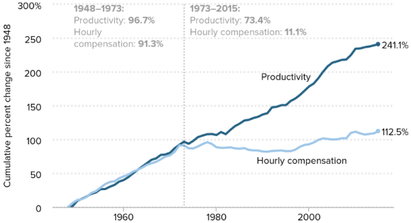
Note: Data are for average hourly compensation of production/nonsupervisory workers in the private sector and net productivity of the total economy. “Net productivity” is the growth of output of goods and services minus depreciation per hour worked.
[324] Report: “Workers’ Compensation: Growing Along with Productivity.” By James Sherk. Heritage Foundation, May, 31, 2016. <report.heritage.org>
Productivity and Pay for Different Workers
A major reason why some studies show a gap between pay and productivity is that they compare different groups of employees and ignore a portion of employees’ compensation. These studies measure the productivity of all employees as well as the self-employed. However, they only consider the compensation of some employees: private-sector “production and non-supervisory employees” covered by the Bureau of Labor Statistics (BLS) payroll survey.17
BLS data show that production and non-supervisory jobs constitute about 63 percent of jobs in the overall economy.18 This category excludes all government employees, the self-employed, and about 20 percent of private-sector firms’ employees. Among the excluded are the majority of the most highly paid workers in America. This makes a large difference: Over the past generation, compensation has risen faster among high earners than in the rest of the economy.
17 The payroll survey measures only wages; it does not include benefits. The Economic Policy Institute imputes benefits to the payroll-survey based wages using data from the National Income and Product Accounts. See Appendix A for details on this imputation and mathematical mistakes that EPI [Economic Policy Institute] makes in doing so.
18 The Bureau of Labor Statistics payroll survey reported 96.8 million production and non-supervisory employees in the private sector in 2014. The BLS household survey reported 146.6 million workers in the total economy. These figures include government employees, the self-employed, private household workers, and farm employees. The payroll survey counts America’s 7.1 million multiple job holders separately at each payroll job they hold, while the household survey counts each employee once, no matter how many jobs he holds. To maintain comparability between the surveys, it is necessary to count multiple job holders in the household survey on the same basis as the payroll survey. This yields 153.7 million jobs in the overall economy, of which 63 percent are production and non-supervisory positions covered by the payroll survey.
[325] Working paper: “Did Wages Reflect Growth in Productivity?” By Martin Feldstein. National Bureau of Economic Research, April 2008. <www.nber.org>
Page 2:
Two principal measurement mistakes have led some analysts to conclude that the rise in labor income has not kept up with the growth in productivity. The first of these is a focus on wages rather than total compensation. Because of the rise in fringe benefits and other noncash payments, wages have not risen as rapidly as total compensation. It is important therefore to compare the productivity rise with the increase of total compensation rather than with the increase of the narrower measure of just wages and salaries.
[326] Article: “Comparing the Consumer Price Index with the Gross Domestic Product Price Index and Gross Domestic Product Implicit Price Deflator.” By Jonathon D. Church. U.S. Department of Labor, Bureau of Labor Statistics Monthly Labor Review, March 2016. <www.bls.gov>
The Consumer Price Index (CPI) and the gross domestic product (GDP) price index and implicit price deflator are measures of inflation in the U.S. economy. The CPI measures price changes in goods and services purchased out of pocket by urban consumers, whereas the GDP price index and implicit price deflator measure price changes in goods and services purchased by consumers, businesses, government, and foreigners, but not importers. Thus, which one to use in a given scenario depends on one’s purpose.
Inflation can be defined as a consistent increase in an economy’s “price level,” or the price component of total expenditures on a set of goods and services, over a given period. The Consumer Price Index (CPI), a product of the Bureau of Labor Statistics (BLS), is perhaps the most widely used measure of inflation in the United States. The CPI measures the average change over time in the prices paid by urban consumers in the United States for a market basket of goods and services.
The Personal Consumption Expenditures (PCE) price index, produced by the U.S. Bureau of Economic Analysis (BEA), is another measure of consumer inflation and is followed closely by the U.S. Board of Governors of the Federal Reserve System (the Federal Reserve). Despite differences in scope, weight, and methodology, the CPI and the PCE price index both measure inflation from the perspective of the consumer. However, one might be interested in an index that measures price change across a broader or narrower range of goods and services—for example, an index that measures price change across a set of goods and services that includes not just consumer goods and services, but also goods and services purchased by businesses, government, and other entities.
One such measure is the price index associated with the nation’s gross domestic product (GDP). Each quarter, BEA releases data on the level of, and change in, GDP. These data include a breakdown of GDP into price and quantity indexes, as well as a GDP implicit price deflator. The GDP price index and implicit price deflator are derived from the measurement of GDP, giving rise to three main issues that distinguish the GDP price indexes from other measures of inflation. The first issue is the scope of goods and services for which prices are collected and indexes are calculated. The second is the weight attached to prices for these goods and services. The third is the methodological details of price index calculation.
[327] Working paper: “Did Wages Reflect Growth in Productivity?” By Martin Feldstein. National Bureau of Economic Research, April 2008. <www.nber.org>
Pages 2–3:
The second measurement problem is the way in which nominal output and nominal compensation are converted to real values before making the comparison. Although any consistent deflation of the two series of nominal values will show similar movements of productivity and compensation, it is misleading in this context to use two different deflators, one for measuring productivity and the other for measuring real compensation.
A quick review of what economic theory says about the relation between productivity and compensation will clarify the correct choice of price deflator for making this comparison and will also indicate how productivity and compensation would be expected to move in a competitive economy. In the classroom we often abstract from differences in prices by assuming an economy with a single product and therefore summarize the basic wage determination condition by saying that a competitive firm pays a wage equal to the marginal product of labor. But when we recognize the multiproduct nature of the economy, we say that the competitive firm pays a nominal wage equal to the marginal revenue product of labor, i.e., to the marginal product of labor multiplied by the price of the firm’s product. The key real relation must therefore be between changes in productivity in the nonfarm business sector and changes in the nominal compensation paid in that sector deflated by the product price and not by some consumer price that also reflects goods and services produced outside the domestic nonfarm business sector.
Pages 4–5:
There are of course other questions for which using compensation deflated by the CPI [Consumer Price Index] or some other consumer price index is appropriate, including measuring changes in the standard of living of wage earners and in the incentive to supply labor. But the nominal compensation deflated by the CPI is not appropriate for evaluating the relation between productivity and compensation.
Page 8: “In summary, basic theory reminds us that real compensation should be
measured using the same price index that is used to calculate productivity.”
[328] Email from the U.S. Bureau of Economic Analysis to Just Facts, February 21, 2017.
Regarding the correct price index to use when comparing output and compensation, for some questions the same index should be used for both. For example, if one is interested in whether workers’ earnings are rising with productivity gains, then it is appropriate to use the same index for both. Note that this is the same comparing compensation and output in nominal terms.
[329] Article: “The Growing Gap Between Real Wages and Labor Productivity.” By Robert Lawrence. Peterson Institute for International Economics, July 21, 2015. <piie.com>
When appropriately measured, from 1970 to 2000, and perhaps to as late as 2008, the growth in overall worker compensation was precisely as rapid as the growth in average labor productivity would imply. This suggests that the key to explaining sluggish long-run wage growth is understanding productivity growth rather than what drives the distribution of income between capital and labor. If there is something about the American economy that has kept workers from maintaining their share in output as the economy expands, this phenomenon has materialized only relatively recently.
First, production and nonsupervisory workers do not constitute the full US labor force. Broader measures that include the wages of all workers show considerably more real wage growth—a reflection of the fact that the wages of more skilled and educated workers grew much more rapidly than blue-collar workers with less education.
[330] Article: “The Compensation–Productivity Gap: A Visual Essay.” By Susan Fleck, John Glaser, and Shawn Sprague. U.S. Department of Labor, Bureau of Labor Statistics Monthly Labor Review, January, 2011. <www.bls.gov>
Page 57:
This visual essay presents real hourly compensation data based on compensation data from the National Income and Product Accounts, which is the same source that the BLS [U.S. Bureau of Labor Statistics ] productivity program uses for output. Compensation data are adjusted by using a consumer price index, and output is adjusted by using an implicit price deflator. …
… Because real hourly compensation and labor productivity, which is output per hour, both include hours worked in their calculations, changes in hours worked have no impact on the gap.
Page 62:
A price index measures the price of a basket of goods and services over time. The Compensation–Productivity gap is partly accounted for by the difference between the two price indexes used to remove the effect of inflation. The implicit price deflator, used to remove the effect of inflation on output, measures price changes in the goods and services produced in the nonfarm business sector. The Consumer Price Index measures price changes in the basket of goods and services purchased by families and workers; it is used to calculate real hourly compensation.
[331] Webpage: “Implicit Price Deflator.” U.S. Department of Commerce, Bureau of Economic Analysis. Last modified January 1, 2023. <www.bea.gov>
“Implicit price deflator (IPD). The ratio of the current-dollar value of a series, such as gross domestic product (GDP), to its corresponding chained-dollar value, multiplied by 100.”
[332] Article: “Comparing the Consumer Price Index with the Gross Domestic Product Price Index and Gross Domestic Product Implicit Price Deflator.” By Jonathon D. Church. U.S. Department of Labor, Bureau of Labor Statistics Monthly Labor Review, March 2016. <www.bls.gov>
The Consumer Price Index (CPI) and the gross domestic product (GDP) price index and implicit price deflator are measures of inflation in the U.S. economy. The CPI measures price changes in goods and services purchased out of pocket by urban consumers, whereas the GDP price index and implicit price deflator measure price changes in goods and services purchased by consumers, businesses, government, and foreigners, but not importers. Thus, which one to use in a given scenario depends on one’s purpose. …
One such measure is the price index associated with the nation’s gross domestic product (GDP). Each quarter, BEA [U.S. Bureau of Economic Analysis] releases data on the level of, and change in, GDP. These data include a breakdown of GDP into price and quantity indexes, as well as a GDP implicit price deflator. The GDP price index and implicit price deflator are derived from the measurement of GDP, giving rise to three main issues that distinguish the GDP price indexes from other measures of inflation. The first issue is the scope of goods and services for which prices are collected and indexes are calculated. The second is the weight attached to prices for these goods and services. The third is the methodological details of price index calculation.
[333] Webpage: “Revised Measure Names and LABSTAT Codes for Labor Productivity and Costs Data.” U.S. Bureau of Labor Statistics. Last modified January 30, 2023. <www.bls.gov>
Effective with the February 2, 2023 Labor Productivity and Costs release, several measure names and series codes will be changing to improve consistency across all productivity products and reflect the data more accurately. ….
Previous Measure Name [=] Implicit price deflator … New Measure Name [=] Value-added output price deflator
[334] Webpage: “Frequently Asked Questions.” U.S. Department of Labor, Bureau of Labor Statistics. Last modified January 18, 2023. <www.bls.gov>
1. What Is the CPI?
The Consumer Price Index (CPI) is a measure of the average change over time in the prices paid by urban consumers for a market basket of consumer goods and services. …
5. How Is the CPI Used?
The CPI affects nearly all Americans because of the many ways it is used. Some examples of how it is used follow:
• As an economic indicator. The CPI is the most widely used measure of inflation and is sometimes viewed as an indicator of the effectiveness of government economic policy. It provides information about price changes in the Nation’s economy to government, business, labor, and private citizens and is used by them as a guide to making economic decisions. In addition, the President, Congress, and the Federal Reserve Board use trends in the CPI to aid in formulating fiscal and monetary policies.
• As a deflator of other economic series. The CPI and its components are used to adjust other economic series for price changes and to translate these series into inflation-free dollars. Examples of series adjusted by the CPI include retail sales, hourly and weekly earnings, and components of the National Income and Product Accounts.
The CPI is also used as a deflator of the value of the consumer’s dollar to find its purchasing power. The purchasing power of the consumer’s dollar measures the change in the value to the consumer of goods and services that a dollar will buy at different dates. In other words, as prices increase, the purchasing power of the consumer’s dollar declines.
• As a means of adjusting dollar values. The CPI is often used to adjust consumers’ income payments (for example, Social Security), to adjust income eligibility levels for government assistance, and to automatically provide cost-of-living wage adjustments to millions of American workers. The index affects the income of more than 90 million people because of statutory action: over 65 million Social Security beneficiaries and over 38 million Supplemental Nutrition Assistance Program (SNAP) recipients (formerly food stamps), among other programs.
Another example of how dollar values may be adjusted is the use of the CPI to adjust the Federal income tax structure. These adjustments prevent inflation-induced increases in tax rates. In addition, eligibility criteria for millions of food stamp recipients, and children who eat lunch at school, are affected by changes in the CPI. Many collective bargaining agreements also tie wage increases to the CPI.
[335] Article: “Comparing the Consumer Price Index with the Gross Domestic Product Price Index and Gross Domestic Product Implicit Price Deflator.” By Jonathon D. Church. U.S. Department of Labor, Bureau of Labor Statistics Monthly Labor Review, March 2016. <www.bls.gov>
The Consumer Price Index (CPI) and the gross domestic product (GDP) price index and implicit price deflator are measures of inflation in the U.S. economy. The CPI measures price changes in goods and services purchased out of pocket by urban consumers, whereas the GDP price index and implicit price deflator measure price changes in goods and services purchased by consumers, businesses, government, and foreigners, but not importers. Thus, which one to use in a given scenario depends on one’s purpose.
[336] Webpage: “US Business Cycle Expansions and Contractions.” National Bureau of Economic Research. Last updated March 14, 2023. <www.nber.org>
“Contractions (recessions) start at the peak of a business cycle and end at the trough. … Peak Month (Peak Quarter) [=] December 2007 (2007Q4) … Trough Month (Trough Quarter) [=] June 2009 (2009Q2)”
[337] “WHO Director-General’s Opening Remarks at the Media Briefing on Covid-19.” World Health Organization, March 11, 2020. <bit.ly>
[Dr. Tedros Adhanom Ghebreyesus:] …
WHO [World Health Organization] has been assessing this outbreak around the clock and we are deeply concerned both by the alarming levels of spread and severity, and by the alarming levels of inaction.
We have therefore made the assessment that COVID-19 can be characterized as a pandemic.
[338] Press release: “COVID-19 and Other Global Health Issues.” World Health Organization, May 5, 2023. <www.justfacts.com>
[Dr. Tedros Adhanom Ghebreyesus:] …
Yesterday, the Emergency Committee met for the 15th time and recommended to me that I declare an end to the public health emergency of international concern. I have accepted that advice. It’s therefore with great hope that I declare COVID-19 over as a global health emergency.
[339] Calculated with data from:
a) Dataset: “Annual Total Factor Productivity and Related Measures, Private Business Sector, 1948–2021.” U.S. Department of Labor, Bureau of Labor Statistics, November 18, 2022. <www.bls.gov>
Tab: “Annual: Annual Total Factor Productivity and Related Measures for Major Industries, Linked SIC-NAICS [Standard Industrial Classification and North American Industrial Classification System]”
b) Dataset: “CPI—All Urban Consumers (Current Series).” U.S. Department of Labor, Bureau of Labor Statistics. Accessed January 27, 2023 at <www.bls.gov>
Series: “CUUR0000SA0. All Items in U.S. City Average, All Urban Consumers, Not Seasonally Adjusted, 1982–84=100”
NOTE: An Excel file containing the data and calculations is available upon request.
[340] Webpage: “Revised Measure Names and LABSTAT Codes for Labor Productivity and Costs Data.” U.S. Bureau of Labor Statistics. Last modified January 30, 2023. <www.bls.gov>
Effective with the February 2, 2023 Labor Productivity and Costs release, several measure names and series codes will be changing to improve consistency across all productivity products and reflect the data more accurately. ….
Previous Measure Name [=] Implicit price deflator … New Measure Name [=] Value-added output price deflator
[341] For facts about these issues, see the sections of this research on the GINI index, marriage, and work.
[342] Webpage: “Listings of WHO’s Response to Covid-19.” World Health Organization, June 29, 2020. Last updated January 29, 2021. <bit.ly>
“11 Mar 2020: Deeply concerned both by the alarming levels of spread and severity, and by the alarming levels of inaction, WHO made the assessment that Covid-19 could be characterized as a pandemic.”
[343] Calculated with the dataset: “The Distribution of Household Income, 2019.” Congressional Budget Office, November 2022. <www.cbo.gov>
“Table 3. Average Household Income, by Income Source and Income Group, 1979 to 2019, 2019 Dollars”
NOTES:
[344] Report: “The Distribution of Household Income, 2019.” Congressional Budget Office, November 2022. <www.cbo.gov>
Pages 33–34:
Data
The core data used in CBO’s [Congressional Budget Office’s] distributional analyses come from the Statistics of Income (SOI), a nationally representative sample of individual income tax returns collected by the Internal Revenue Service (IRS). The number of returns sampled grew over the period studied—1979 to 2019—rising from roughly 90,000 in some of the early years to more than 350,000 in later years. That sample of tax returns becomes available to CBO approximately two years after the returns are filed. …
Information from tax returns is supplemented with data from the Annual Social and Economic Supplement of the Census Bureau’s Current Population Survey (CPS), which contains survey data on the demographic characteristics and income of a large sample of households.5 The two sources are combined by statistically matching each SOI record to a corresponding CPS record on the basis of demographic characteristics and income. Each pairing results in a new record that takes on some characteristics of the CPS record and some characteristics of the SOI record.6
Page 35:
Measures of Income, Federal Taxes, and Means-Tested Transfers
Most distributional analyses rely on a measure of annual income as the metric for ranking households. In CBO’s analyses, information on taxable income sources for tax-filing units that file individual income tax returns comes from the SOI, whereas information on nontaxable income sources and income for tax-filing units that do not file individual income tax returns comes from the CPS. Among households at the top of the distribution, the majority of income data are drawn from the SOI. In contrast, among households in the lower and middle quintiles, a larger portion of income data is drawn from the CPS….
Pages 39–40:
Household income, unless otherwise indicated, refers to income before accounting for the effects of means-tested transfers and federal taxes. Throughout this report, that income concept is called income before transfers and taxes. It consists of market income plus social insurance benefits.
Market income consists of the following:
• Labor income. Wages and salaries, including those allocated by employees to 401(k) and other employment-based retirement plans; employer-paid health insurance premiums (as measured by the Census Bureau’s Current Population Survey); the employer’s share of Social Security, Medicare, and federal unemployment insurance payroll taxes; and the share of corporate income taxes borne by workers.
• Business income. Net income from businesses and farms operated solely by their owners, partnership income, and income from S corporations.
• Capital income (including capital gains). Net profits realized from the sale of assets (but not increases in the value of assets that have not been realized through sales); taxable and tax-exempt interest; dividends paid by corporations (but not dividends from S corporations, which are considered part of business income); positive rental income; and the share of corporate income taxes borne by capital owners.†
• Other income sources. Income received in retirement for past services and other nongovernmental sources of income.
Social insurance benefits consist of benefits from Social Security (Old Age, Survivors, and Disability Insurance), Medicare (measured by the average cost to the government of providing those benefits), unemployment insurance, and workers’ compensation.
Means-tested transfers are cash payments and in-kind services provided through federal, state, and local government assistance programs. Eligibility to receive such transfers is determined primarily on the basis of income, which must be below certain thresholds. Means-tested transfers are provided through the following programs: Medicaid and the Children’s Health Insurance Program (measured by the average cost to the government of providing those benefits); the Supplemental Nutrition Assistance Program (formerly known as the Food Stamp program); housing assistance programs; Supplemental Security Income; Temporary Assistance for Needy Families and its predecessor, Aid to Families With Dependent Children; child nutrition programs; the Low Income Home Energy Assistance Program; and state and local government general assistance programs.
Average means-tested transfer rates are calculated as means-tested transfers divided by income before transfers and taxes.
Federal taxes consist of individual income taxes, payroll (or social insurance) taxes, corporate income taxes, and excise taxes. Those four sources accounted for 93 percent of federal revenues in fiscal year 2019. Revenue sources not examined in this report include states’ deposits for unemployment insurance, estate and gift taxes, net income of the Federal Reserve System that is remitted to the Treasury, customs duties, and miscellaneous fees and fines.
In this analysis, taxes for a given year are the amount a household owes on the basis of income received that year, regardless of when the taxes are paid. Those taxes comprise the following:
• Individual income taxes. Individual income taxes are paid by U.S. citizens and residents on their income from all sources, except those sources exempted under the law. Individual income taxes can be negative because they include the effects of refundable tax credits, which can result in net payments from the government. Specifically, if the amount of a refundable tax credit exceeds a filer’s tax liability before the credit is applied, the government pays that excess to the filer. Statutory marginal individual income tax rates are the rates set in law that apply to the last dollar of income.
• Payroll taxes. Payroll taxes are levied primarily on wages and salaries and generally have a single rate and few exclusions, deductions, or credits. Payroll taxes include those that fund the Social Security trust funds, the Medicare trust fund, and unemployment insurance trust funds. The federal portion of the unemployment insurance payroll tax covers only administrative costs for the program; state-collected unemployment insurance payroll taxes are not included in the Congressional Budget Office’s measure of federal taxes (even though they are recorded as revenues in the federal budget). Households can be entitled to future social insurance benefits, including Social Security, Medicare, and unemployment insurance, as a result of paying payroll taxes. In this analysis, average payroll tax rates capture the taxes paid in a given year and do not capture the benefits households may receive in the future.
• Corporate income taxes. Corporate income taxes are levied on the profits of U.S.-based corporations organized as C corporations. In its analysis, CBO allocated 75 percent of corporate income taxes in proportion to each household’s share of total capital income (including capital gains) and 25 percent to households in proportion to their share of labor income.
• Excise taxes. Sales of a wide variety of goods and services are subject to federal excise taxes. Most revenues from excise taxes are attributable to the sale of motor fuels (gasoline and diesel fuel), tobacco products, alcoholic beverages, and aviation-related goods and services (such as aviation fuel and airline tickets).
Average federal tax rates are calculated as federal taxes divided by income before transfers and taxes.
Income after transfers and taxes is income before transfers and taxes plus means-tested transfers minus federal taxes.
Income groups are created by ranking households by their size-adjusted income before transfers and taxes. A household consists of people sharing a housing unit, regardless of their relationships. The income quintiles (fifths) contain approximately the same number of people but slightly different numbers of households…. Similarly, each full percentile (hundredth) contains approximately the same number of people but a different number of households. If a household has negative income (that is, if its business or investment losses are larger than its other income), it is excluded from the lowest income group but included in totals.
NOTE: † See Just Facts’ research on the distribution of the federal tax burden for details about how the Congressional Budget Office determines the share of corporate income taxes borne by workers and owners of capital.
[345] Article: “How Many Workers Are Employed in Sectors Directly Affected by Covid-19 Shutdowns, Where Do They Work, and How Much Do They Earn?” By Matthew Dey and Mark A. Loewenstein. U.S. Bureau of Labor Statistics Monthly Labor Review, April 2020. <www.bls.gov>
Page 1: “To reduce the spread of coronavirus disease 2019 (Covid-19), nearly all states have issued stay-at-home orders and shut down establishments deemed nonessential.”
[346] Article: “Covid-19 Restrictions.” USA Today. Last updated July 11, 2022. <www.usatoday.com>
Throughout the pandemic, officials across the United States have rolled out a patchwork of restrictions on social distancing, masking and other aspects of public life. The orders vary by state, county and even city. At the height of restrictions in late March and early April 2020, more than 310 million Americans were under directives ranging from “shelter in place” to “stay at home.” Restrictions are now ramping down in many places, as most states have fully reopened their economies.
[347] During 2020 and early 2021, federal politicians enacted six “Covid relief” laws that will cost a total of about $5.2 trillion over the course of a decade. This amounts to an average of $40,444 in spending per U.S. household.
Calculated with data from:
a) Report: “CBO Estimate for H.R. 6074, the Coronavirus Preparedness and Response Supplemental Appropriations Act, 2020, as Posted on March 4, 2020.” Congressional Budget Office, March 4, 2020. <www.cbo.gov>
b) Report: “Cost Estimate for H.R. 6201, Families First Coronavirus Response Act, Enacted as Public Law 116-127 on March 18, 2020.” Congressional Budget Office, April 2, 2020. <www.cbo.gov>
c) Report: “Cost Estimate for H.R. 748, CARES Act, Public Law 116-136.” Congressional Budget Office, April 16, 2020. <www.cbo.gov>
d) Report: “CBO Estimate for H.R. 266, the Paycheck Protection Program and Health Care Enhancement Act as Passed by the Senate on April 21, 2020.” Congressional Budget Office, April 22, 2020. <www.cbo.gov>
e) Report: “Estimate for Division N—Additional Coronavirus Response and Relief, H.R. 133, Consolidated Appropriations Act, 2021, Public Law 116-260, Enacted on December 27, 2020.” Congressional Budget Office, January 14, 2021. <www.cbo.gov>
f) Report: “Estimated Budgetary Effects of H.R. 1319, American Rescue Plan Act of 2021 as Passed by the Senate on March 6, 2021.” Congressional Budget Office, March 10, 2021. <www.cbo.gov>
g) Dataset: “HH-1. Households by Type: 1940 to Present.” U.S. Census Bureau, Current Population Survey, November 2021. <www.census.gov>
NOTE: An Excel file containing the data and calculations is available upon request.
[348] Calculated with the dataset: “The Distribution of Household Income, 2020.” Congressional Budget Office, November 2023. <www.cbo.gov>
“Table 3. Average Household Income, by Income Source and Income Group, 1979 to 2020, 2020 Dollars”
NOTES:
[349] Report: “The Distribution of Household Income, 2020.” Congressional Budget Office, November 2023. <www.cbo.gov>
Page 20:
Data
The core data used in CBO’s distributional analyses come from the Statistics of Income (SOI), a nationally representative sample of individual income tax returns collected by the IRS. That sample of tax returns becomes available to CBO approximately two years after the returns are filed. Data on household income are systematically and consistently reported in the SOI. The sample is therefore considered a reliable resource to use when analyzing the effects of fiscal policy on income. However, certain types of income are not reported in the SOI. In 2020, for example, the portion of payments from the Paycheck Protection Program that was not used to pay for employees’ wages was not taxable and therefore not available in the SOI data.
SOI data include information about tax filers’ family structure and age, but they do not include certain demographic information or data on people who do not file taxes. For that information, CBO uses data from the Annual Social and Economic Supplement of the Census Bureau’s Current Population Survey (CPS), which has data on the demographic characteristics and income of a large sample of households.6
CBO combines the two data sources, statistically matching each SOI record to a corresponding CPS record on the basis of demographic characteristics and income. Each pairing results in a new record that takes on some characteristics of the CPS record and some characteristics of the SOI record.7
Page 22:
Measures of Income, Federal Taxes, and Means-Tested Transfers
Most distributional analyses rely on a measure of annual income as the metric for ranking households. In CBO’s analyses of the distribution of household income, information about taxable income sources for tax-filing units that file individual income tax returns comes from the SOI, whereas information about nontaxable income sources and income for tax-filing units that do not file individual income tax returns comes from the CPS. Among households at the top of the income distribution, the majority of income data are drawn from the SOI. In contrast, among households in the lower and middle quintiles, a larger portion of income data is drawn from the CPS….
Pages 31–32:
Household income, unless otherwise indicated, refers to income before the effects of means-tested transfers and federal taxes are accounted for. Throughout this report, that income concept is called income before transfers and taxes. It consists of market income plus social insurance benefits.
Market income consists of the following five elements:
• Labor income. Wages and salaries, including those allocated by employees to 401(k) and other employment-based retirement plans; employer-paid health insurance premiums (as measured by the Census Bureau’s Current Population Survey); the employer’s share of payroll taxes for Social Security, Medicare, and federal unemployment insurance; and the share of corporate income taxes borne by workers.
• Business income. Net income from businesses and farms operated solely by their owners, partnership income, and income from S corporations.
• Capital gains. Net profits realized from the sale of assets (but not increases in the value of assets that have not been realized through sales).
• Capital income. Taxable and tax-exempt interest, dividends paid by corporations (but not dividends from S corporations, which are considered part of business income), rental income, and the share of corporate income taxes borne by capital owners.
• Other income sources. Income received in retirement for past services and other nongovernmental sources of income.
Social insurance benefits consist of benefits from Social Security (Old Age, Survivors, and Disability Insurance), Medicare (measured by the average cost to the government of providing those benefits), regular unemployment insurance (but not expanded unemployment compensation), and workers’ compensation.
Means-tested transfers are cash payments and in-kind services provided through federal, state, and local government assistance programs. Eligibility to receive such transfers is determined primarily on the basis of income, which must be below certain thresholds. Means-tested transfers are provided through the following programs: Medicaid and the Children’s Health Insurance Program (measured by the average cost to the federal government and state governments of providing those benefits); the Supplemental Nutrition Assistance Program (formerly known as the Food Stamp program); housing assistance programs; Supplemental Security Income; Temporary Assistance for Needy Families and its predecessor, Aid to Families With Dependent Children; child nutrition programs; the Low Income Home Energy Assistance Program; and state and local governments’ general assistance programs. For 2020, CBO included expanded unemployment compensation in means-tested transfers.
Average means-tested transfer rates are calculated as means-tested transfers (totaled within an income group) divided by income before transfers and taxes (totaled within an income group).
Federal taxes consist of individual income taxes, payroll (or social insurance) taxes, corporate income taxes, and excise taxes. Those four sources accounted for 94 percent of federal revenues in fiscal year 2020. Revenue sources not examined in this report include states’ deposits for unemployment insurance, estate and gift taxes, net income of the Federal Reserve System that is remitted to the Treasury, customs duties, and miscellaneous fees and fines.
In this analysis, taxes for a given year are the amount a household owes on the basis of income received in that year, regardless of when the taxes are paid. Those taxes comprise the following four categories:
• Individual income taxes. Individual income taxes are levied on income from all sources, except those excluded by law. Individual income taxes can be negative because they include the effects of refundable tax credits (including recovery rebate credits), which can result in net payments from the government. Specifically, if the amount of a refundable tax credit exceeds a filer’s tax liability before the credit is applied, the government pays that excess to the filer. Statutory marginal individual income tax rates are the rates set in law that apply to the last dollar of income.
• Payroll taxes. Payroll taxes are levied primarily on wages and salaries. They generally have a single rate and few exclusions, deductions, or credits. Payroll taxes include those that fund the Social Security trust funds, the Medicare trust fund, and unemployment insurance trust funds. The federal portion of the unemployment insurance payroll tax covers only administrative costs for the program; state-collected unemployment insurance payroll taxes are not included in the Congressional Budget Office’s measure of federal taxes (even though they are recorded as revenues in the federal budget). Households can be entitled to future social insurance benefits, including Social Security, Medicare, and unemployment insurance, as a result of paying payroll taxes. In this analysis, average payroll tax rates capture the taxes paid in a given year and do not capture the benefits that households may receive in the future.
• Corporate income taxes. Corporate income taxes are levied on the profits of U.S.–based corporations organized as C corporations. In this analysis, CBO allocated 75 percent of corporate income taxes in proportion to each household’s share of total capital income (including capital gains) and 25 percent to households in proportion to their share of labor income.
• Excise taxes. Sales of a wide variety of goods and services are subject to federal excise taxes. Most revenues from excise taxes are attributable to the sale of motor fuels (gasoline and diesel fuel), tobacco products, alcoholic beverages, and aviation-related goods and services (such as aviation fuel and airline tickets).
Average federal tax rates are calculated as federal taxes (totaled within an income group) divided by income before transfers and taxes (totaled within an income group).
Income after transfers and taxes is income before transfers and taxes plus means-tested transfers minus federal taxes.
Income groups are created by ranking households by their size-adjusted income before transfers and taxes. A household consists of people sharing a housing unit, regardless of their relationship. The income quintiles (or fifths of the distribution) contain approximately the same number of people but slightly different numbers of households…. Similarly, each full percentile (or hundredth of the distribution) contains approximately the same number of people but a different number of households. If a household has negative income (that is, if its business or investment losses exceed its other income), it is excluded from the lowest income group but included in totals.
NOTE: † See Just Facts’ research on the distribution of the federal tax burden for details about how the Congressional Budget Office determines the share of corporate income taxes borne by workers and owners of capital.
[350] Webpage: “Listings of WHO’s Response to Covid-19.” World Health Organization, June 29, 2020. Last updated January 29, 2021. <bit.ly>
“11 Mar 2020: Deeply concerned both by the alarming levels of spread and severity, and by the alarming levels of inaction, WHO made the assessment that Covid-19 could be characterized as a pandemic.”
[351] Calculated with the dataset: “The Distribution of Household Income, 2019.” Congressional Budget Office, November 2022. <www.cbo.gov>
“Table 3. Average Household Income, by Income Source and Income Group, 1979 to 2019, 2019 Dollars”
NOTES:
[352] Report: “The Distribution of Household Income, 2019.” Congressional Budget Office, November 2022. <www.cbo.gov>
Pages 33–34:
Data
The core data used in CBO’s [Congressional Budget Office’s] distributional analyses come from the Statistics of Income (SOI), a nationally representative sample of individual income tax returns collected by the Internal Revenue Service (IRS). The number of returns sampled grew over the period studied—1979 to 2019—rising from roughly 90,000 in some of the early years to more than 350,000 in later years. That sample of tax returns becomes available to CBO approximately two years after the returns are filed. …
Information from tax returns is supplemented with data from the Annual Social and Economic Supplement of the Census Bureau’s Current Population Survey (CPS), which contains survey data on the demographic characteristics and income of a large sample of households.5 The two sources are combined by statistically matching each SOI record to a corresponding CPS record on the basis of demographic characteristics and income. Each pairing results in a new record that takes on some characteristics of the CPS record and some characteristics of the SOI record.6
Page 35:
Measures of Income, Federal Taxes, and Means-Tested Transfers
Most distributional analyses rely on a measure of annual income as the metric for ranking households. In CBO’s analyses, information on taxable income sources for tax-filing units that file individual income tax returns comes from the SOI, whereas information on nontaxable income sources and income for tax-filing units that do not file individual income tax returns comes from the CPS. Among households at the top of the distribution, the majority of income data are drawn from the SOI. In contrast, among households in the lower and middle quintiles, a larger portion of income data is drawn from the CPS….
Pages 39–40:
Household income, unless otherwise indicated, refers to income before accounting for the effects of means-tested transfers and federal taxes. Throughout this report, that income concept is called income before transfers and taxes. It consists of market income plus social insurance benefits.
Market income consists of the following:
• Labor income. Wages and salaries, including those allocated by employees to 401(k) and other employment-based retirement plans; employer-paid health insurance premiums (as measured by the Census Bureau’s Current Population Survey); the employer’s share of Social Security, Medicare, and federal unemployment insurance payroll taxes; and the share of corporate income taxes borne by workers.
• Business income. Net income from businesses and farms operated solely by their owners, partnership income, and income from S corporations.
• Capital income (including capital gains). Net profits realized from the sale of assets (but not increases in the value of assets that have not been realized through sales); taxable and tax-exempt interest; dividends paid by corporations (but not dividends from S corporations, which are considered part of business income); positive rental income; and the share of corporate income taxes borne by capital owners.†
• Other income sources. Income received in retirement for past services and other nongovernmental sources of income.
Social insurance benefits consist of benefits from Social Security (Old Age, Survivors, and Disability Insurance), Medicare (measured by the average cost to the government of providing those benefits), unemployment insurance, and workers’ compensation.
Means-tested transfers are cash payments and in-kind services provided through federal, state, and local government assistance programs. Eligibility to receive such transfers is determined primarily on the basis of income, which must be below certain thresholds. Means-tested transfers are provided through the following programs: Medicaid and the Children’s Health Insurance Program (measured by the average cost to the government of providing those benefits); the Supplemental Nutrition Assistance Program (formerly known as the Food Stamp program); housing assistance programs; Supplemental Security Income; Temporary Assistance for Needy Families and its predecessor, Aid to Families With Dependent Children; child nutrition programs; the Low Income Home Energy Assistance Program; and state and local government general assistance programs.
Average means-tested transfer rates are calculated as means-tested transfers divided by income before transfers and taxes.
Federal taxes consist of individual income taxes, payroll (or social insurance) taxes, corporate income taxes, and excise taxes. Those four sources accounted for 93 percent of federal revenues in fiscal year 2019. Revenue sources not examined in this report include states’ deposits for unemployment insurance, estate and gift taxes, net income of the Federal Reserve System that is remitted to the Treasury, customs duties, and miscellaneous fees and fines.
In this analysis, taxes for a given year are the amount a household owes on the basis of income received that year, regardless of when the taxes are paid. Those taxes comprise the following:
• Individual income taxes. Individual income taxes are paid by U.S. citizens and residents on their income from all sources, except those sources exempted under the law. Individual income taxes can be negative because they include the effects of refundable tax credits, which can result in net payments from the government. Specifically, if the amount of a refundable tax credit exceeds a filer’s tax liability before the credit is applied, the government pays that excess to the filer. Statutory marginal individual income tax rates are the rates set in law that apply to the last dollar of income.
• Payroll taxes. Payroll taxes are levied primarily on wages and salaries and generally have a single rate and few exclusions, deductions, or credits. Payroll taxes include those that fund the Social Security trust funds, the Medicare trust fund, and unemployment insurance trust funds. The federal portion of the unemployment insurance payroll tax covers only administrative costs for the program; state-collected unemployment insurance payroll taxes are not included in the Congressional Budget Office’s measure of federal taxes (even though they are recorded as revenues in the federal budget). Households can be entitled to future social insurance benefits, including Social Security, Medicare, and unemployment insurance, as a result of paying payroll taxes. In this analysis, average payroll tax rates capture the taxes paid in a given year and do not capture the benefits households may receive in the future.
• Corporate income taxes. Corporate income taxes are levied on the profits of U.S.-based corporations organized as C corporations. In its analysis, CBO allocated 75 percent of corporate income taxes in proportion to each household’s share of total capital income (including capital gains) and 25 percent to households in proportion to their share of labor income.
• Excise taxes. Sales of a wide variety of goods and services are subject to federal excise taxes. Most revenues from excise taxes are attributable to the sale of motor fuels (gasoline and diesel fuel), tobacco products, alcoholic beverages, and aviation-related goods and services (such as aviation fuel and airline tickets).
Average federal tax rates are calculated as federal taxes divided by income before transfers and taxes.
Income after transfers and taxes is income before transfers and taxes plus means-tested transfers minus federal taxes.
Income groups are created by ranking households by their size-adjusted income before transfers and taxes. A household consists of people sharing a housing unit, regardless of their relationships. The income quintiles (fifths) contain approximately the same number of people but slightly different numbers of households…. Similarly, each full percentile (hundredth) contains approximately the same number of people but a different number of households. If a household has negative income (that is, if its business or investment losses are larger than its other income), it is excluded from the lowest income group but included in totals.
NOTE: † See Just Facts’ research on the distribution of the federal tax burden for details about how the Congressional Budget Office determines the share of corporate income taxes borne by workers and owners of capital.
[353] Economists typically use a “comprehensive measure of income” to calculate effective tax rates, because this provides a complete “measure of ability to pay” taxes.† In keeping with this, Just Facts determines effective tax rates by dividing all measurable taxes by all income. The Congressional Budget Office (CBO) previously did the same,‡ but in 2018, CBO announced that it would exclude means-tested transfers from its measures of income and effective tax rates.§ #
Given this change, Just Facts now uses CBO data to determine comprehensive income and effective tax rates by adding back the means-tested transfers that CBO publishes but takes out of these measures. To do this, Just Facts makes a simplifying assumption that households in various income quintiles do not significantly change when these transfers are added. This is mostly true, but as CBO notes:
Almost one-fifth of the households in the lowest quintile of income before transfers and taxes would have been in higher quintiles if means-tested transfers were included in the ranking measure (see Table 5). Because net movement into a higher income quintile entails a corresponding net movement out of those quintiles, more than one-fifth of the households in the second quintile of income before transfers and taxes would have been bumped down into the bottom before-tax income quintile. Because before-tax income excludes income in the form of means-tested transfers, almost one-fifth of the people in the lowest quintile of income before transfers and taxes were in higher before-tax income quintiles. There is no fundamental economic change represented by those changes in income groups—just a change in the income definition used to rank households. Because means-tested transfers predominantly go to households in the lower income quintiles, there is not much shuffling across income quintile thresholds toward the top of the distribution.§
NOTES:
[354] Article: “How Many Workers Are Employed in Sectors Directly Affected by Covid-19 Shutdowns, Where Do They Work, and How Much Do They Earn?” By Matthew Dey and Mark A. Loewenstein. U.S. Bureau of Labor Statistics Monthly Labor Review, April 2020. <www.bls.gov>
Page 1: “To reduce the spread of coronavirus disease 2019 (Covid-19), nearly all states have issued stay-at-home orders and shut down establishments deemed nonessential.”
[355] Article: “Covid-19 Restrictions.” USA Today. Last updated July 11, 2022. <www.usatoday.com>
Throughout the pandemic, officials across the United States have rolled out a patchwork of restrictions on social distancing, masking and other aspects of public life. The orders vary by state, county and even city. At the height of restrictions in late March and early April 2020, more than 310 million Americans were under directives ranging from “shelter in place” to “stay at home.” Restrictions are now ramping down in many places, as most states have fully reopened their economies.
[356] During 2020 and early 2021, federal politicians enacted six “Covid relief” laws that will cost a total of about $5.2 trillion over the course of a decade. This amounts to an average of $40,444 in spending per U.S. household.
Calculated with data from:
a) Report: “CBO Estimate for H.R. 6074, the Coronavirus Preparedness and Response Supplemental Appropriations Act, 2020, as Posted on March 4, 2020.” Congressional Budget Office, March 4, 2020. <www.cbo.gov>
b) Report: “Cost Estimate for H.R. 6201, Families First Coronavirus Response Act, Enacted as Public Law 116-127 on March 18, 2020.” Congressional Budget Office, April 2, 2020. <www.cbo.gov>
c) Report: “Cost Estimate for H.R. 748, CARES Act, Public Law 116-136.” Congressional Budget Office, April 16, 2020. <www.cbo.gov>
d) Report: “CBO Estimate for H.R. 266, the Paycheck Protection Program and Health Care Enhancement Act as Passed by the Senate on April 21, 2020.” Congressional Budget Office, April 22, 2020. <www.cbo.gov>
e) Report: “Estimate for Division N—Additional Coronavirus Response and Relief, H.R. 133, Consolidated Appropriations Act, 2021, Public Law 116-260, Enacted on December 27, 2020.” Congressional Budget Office, January 14, 2021. <www.cbo.gov>
f) Report: “Estimated Budgetary Effects of H.R. 1319, American Rescue Plan Act of 2021 as Passed by the Senate on March 6, 2021.” Congressional Budget Office, March 10, 2021. <www.cbo.gov>
g) Dataset: “HH-1. Households by Type: 1940 to Present.” U.S. Census Bureau, Current Population Survey, November 2021. <www.census.gov>
NOTE: An Excel file containing the data and calculations is available upon request.
[357] Calculated with the dataset: “The Distribution of Household Income, 2020.” Congressional Budget Office, November 2023. <www.cbo.gov>
“Table 3. Average Household Income, by Income Source and Income Group, 1979 to 2020, 2020 Dollars”
NOTES:
[358] Report: “The Distribution of Household Income, 2020.” Congressional Budget Office, November 2023. <www.cbo.gov>
Page 20:
Data
The core data used in CBO’s distributional analyses come from the Statistics of Income (SOI), a nationally representative sample of individual income tax returns collected by the IRS. That sample of tax returns becomes available to CBO approximately two years after the returns are filed. Data on household income are systematically and consistently reported in the SOI. The sample is therefore considered a reliable resource to use when analyzing the effects of fiscal policy on income. However, certain types of income are not reported in the SOI. In 2020, for example, the portion of payments from the Paycheck Protection Program that was not used to pay for employees’ wages was not taxable and therefore not available in the SOI data.
SOI data include information about tax filers’ family structure and age, but they do not include certain demographic information or data on people who do not file taxes. For that information, CBO uses data from the Annual Social and Economic Supplement of the Census Bureau’s Current Population Survey (CPS), which has data on the demographic characteristics and income of a large sample of households.6
CBO combines the two data sources, statistically matching each SOI record to a corresponding CPS record on the basis of demographic characteristics and income. Each pairing results in a new record that takes on some characteristics of the CPS record and some characteristics of the SOI record.7
Page 22:
Measures of Income, Federal Taxes, and Means-Tested Transfers
Most distributional analyses rely on a measure of annual income as the metric for ranking households. In CBO’s analyses of the distribution of household income, information about taxable income sources for tax-filing units that file individual income tax returns comes from the SOI, whereas information about nontaxable income sources and income for tax-filing units that do not file individual income tax returns comes from the CPS. Among households at the top of the income distribution, the majority of income data are drawn from the SOI. In contrast, among households in the lower and middle quintiles, a larger portion of income data is drawn from the CPS….
Pages 31–32:
Household income, unless otherwise indicated, refers to income before the effects of means-tested transfers and federal taxes are accounted for. Throughout this report, that income concept is called income before transfers and taxes. It consists of market income plus social insurance benefits.
Market income consists of the following five elements:
• Labor income. Wages and salaries, including those allocated by employees to 401(k) and other employment-based retirement plans; employer-paid health insurance premiums (as measured by the Census Bureau’s Current Population Survey); the employer’s share of payroll taxes for Social Security, Medicare, and federal unemployment insurance; and the share of corporate income taxes borne by workers.
• Business income. Net income from businesses and farms operated solely by their owners, partnership income, and income from S corporations.
• Capital gains. Net profits realized from the sale of assets (but not increases in the value of assets that have not been realized through sales).
• Capital income. Taxable and tax-exempt interest, dividends paid by corporations (but not dividends from S corporations, which are considered part of business income), rental income, and the share of corporate income taxes borne by capital owners.
• Other income sources. Income received in retirement for past services and other nongovernmental sources of income.
Social insurance benefits consist of benefits from Social Security (Old Age, Survivors, and Disability Insurance), Medicare (measured by the average cost to the government of providing those benefits), regular unemployment insurance (but not expanded unemployment compensation), and workers’ compensation.
Means-tested transfers are cash payments and in-kind services provided through federal, state, and local government assistance programs. Eligibility to receive such transfers is determined primarily on the basis of income, which must be below certain thresholds. Means-tested transfers are provided through the following programs: Medicaid and the Children’s Health Insurance Program (measured by the average cost to the federal government and state governments of providing those benefits); the Supplemental Nutrition Assistance Program (formerly known as the Food Stamp program); housing assistance programs; Supplemental Security Income; Temporary Assistance for Needy Families and its predecessor, Aid to Families With Dependent Children; child nutrition programs; the Low Income Home Energy Assistance Program; and state and local governments’ general assistance programs. For 2020, CBO included expanded unemployment compensation in means-tested transfers.
Average means-tested transfer rates are calculated as means-tested transfers (totaled within an income group) divided by income before transfers and taxes (totaled within an income group).
Federal taxes consist of individual income taxes, payroll (or social insurance) taxes, corporate income taxes, and excise taxes. Those four sources accounted for 94 percent of federal revenues in fiscal year 2020. Revenue sources not examined in this report include states’ deposits for unemployment insurance, estate and gift taxes, net income of the Federal Reserve System that is remitted to the Treasury, customs duties, and miscellaneous fees and fines.
In this analysis, taxes for a given year are the amount a household owes on the basis of income received in that year, regardless of when the taxes are paid. Those taxes comprise the following four categories:
• Individual income taxes. Individual income taxes are levied on income from all sources, except those excluded by law. Individual income taxes can be negative because they include the effects of refundable tax credits (including recovery rebate credits), which can result in net payments from the government. Specifically, if the amount of a refundable tax credit exceeds a filer’s tax liability before the credit is applied, the government pays that excess to the filer. Statutory marginal individual income tax rates are the rates set in law that apply to the last dollar of income.
• Payroll taxes. Payroll taxes are levied primarily on wages and salaries. They generally have a single rate and few exclusions, deductions, or credits. Payroll taxes include those that fund the Social Security trust funds, the Medicare trust fund, and unemployment insurance trust funds. The federal portion of the unemployment insurance payroll tax covers only administrative costs for the program; state-collected unemployment insurance payroll taxes are not included in the Congressional Budget Office’s measure of federal taxes (even though they are recorded as revenues in the federal budget). Households can be entitled to future social insurance benefits, including Social Security, Medicare, and unemployment insurance, as a result of paying payroll taxes. In this analysis, average payroll tax rates capture the taxes paid in a given year and do not capture the benefits that households may receive in the future.
• Corporate income taxes. Corporate income taxes are levied on the profits of U.S.–based corporations organized as C corporations. In this analysis, CBO allocated 75 percent of corporate income taxes in proportion to each household’s share of total capital income (including capital gains) and 25 percent to households in proportion to their share of labor income.
• Excise taxes. Sales of a wide variety of goods and services are subject to federal excise taxes. Most revenues from excise taxes are attributable to the sale of motor fuels (gasoline and diesel fuel), tobacco products, alcoholic beverages, and aviation-related goods and services (such as aviation fuel and airline tickets).
Average federal tax rates are calculated as federal taxes (totaled within an income group) divided by income before transfers and taxes (totaled within an income group).
Income after transfers and taxes is income before transfers and taxes plus means-tested transfers minus federal taxes.
Income groups are created by ranking households by their size-adjusted income before transfers and taxes. A household consists of people sharing a housing unit, regardless of their relationship. The income quintiles (or fifths of the distribution) contain approximately the same number of people but slightly different numbers of households…. Similarly, each full percentile (or hundredth of the distribution) contains approximately the same number of people but a different number of households. If a household has negative income (that is, if its business or investment losses exceed its other income), it is excluded from the lowest income group but included in totals.
NOTE: † See Just Facts’ research on the distribution of the federal tax burden for details about how the Congressional Budget Office determines the share of corporate income taxes borne by workers and owners of capital.
[359] Economists typically use a “comprehensive measure of income” to calculate effective tax rates, because this provides a complete “measure of ability to pay” taxes.† In keeping with this, Just Facts determines effective tax rates by dividing all measurable taxes by all income. The Congressional Budget Office (CBO) previously did the same,‡ but in 2018, CBO announced that it would exclude means-tested transfers from its measures of income and effective tax rates.§ #
Given this change, Just Facts now uses CBO data to determine comprehensive income and effective tax rates by adding back the means-tested transfers that CBO publishes but takes out of these measures. To do this, Just Facts makes a simplifying assumption that households in various income quintiles do not significantly change when these transfers are added. This is mostly true, but as CBO notes:
Almost one-fifth of the households in the lowest quintile of income before transfers and taxes would have been in higher quintiles if means-tested transfers were included in the ranking measure (see Table 5). Because net movement into a higher income quintile entails a corresponding net movement out of those quintiles, more than one-fifth of the households in the second quintile of income before transfers and taxes would have been bumped down into the bottom before-tax income quintile. Because before-tax income excludes income in the form of means-tested transfers, almost one-fifth of the people in the lowest quintile of income before transfers and taxes were in higher before-tax income quintiles. There is no fundamental economic change represented by those changes in income groups—just a change in the income definition used to rank households. Because means-tested transfers predominantly go to households in the lower income quintiles, there is not much shuffling across income quintile thresholds toward the top of the distribution.§
NOTES:
[360] Webpage: “Listings of WHO’s Response to Covid-19.” World Health Organization, June 29, 2020. Last updated January 29, 2021. <bit.ly>
“11 Mar 2020: Deeply concerned both by the alarming levels of spread and severity, and by the alarming levels of inaction, WHO made the assessment that Covid-19 could be characterized as a pandemic.”
[361] Calculated with the dataset: “The Distribution of Household Income, 2019.” Congressional Budget Office, November 2022. <www.cbo.gov>
“Table 10. Shares of Household Income, by Income Group, 1979 to 2019 (Percent)”
NOTES:
[362] Report: “The Distribution of Household Income, 2019.” Congressional Budget Office, November 2022. <www.cbo.gov>
Pages 33–34:
Data
The core data used in CBO’s [Congressional Budget Office’s] distributional analyses come from the Statistics of Income (SOI), a nationally representative sample of individual income tax returns collected by the Internal Revenue Service (IRS). The number of returns sampled grew over the period studied—1979 to 2019—rising from roughly 90,000 in some of the early years to more than 350,000 in later years. That sample of tax returns becomes available to CBO approximately two years after the returns are filed. …
Information from tax returns is supplemented with data from the Annual Social and Economic Supplement of the Census Bureau’s Current Population Survey (CPS), which contains survey data on the demographic characteristics and income of a large sample of households.5 The two sources are combined by statistically matching each SOI record to a corresponding CPS record on the basis of demographic characteristics and income. Each pairing results in a new record that takes on some characteristics of the CPS record and some characteristics of the SOI record.6
Page 35:
Measures of Income, Federal Taxes, and Means-Tested Transfers
Most distributional analyses rely on a measure of annual income as the metric for ranking households. In CBO’s analyses, information on taxable income sources for tax-filing units that file individual income tax returns comes from the SOI, whereas information on nontaxable income sources and income for tax-filing units that do not file individual income tax returns comes from the CPS. Among households at the top of the distribution, the majority of income data are drawn from the SOI. In contrast, among households in the lower and middle quintiles, a larger portion of income data is drawn from the CPS….
Pages 39–40:
Household income, unless otherwise indicated, refers to income before accounting for the effects of means-tested transfers and federal taxes. Throughout this report, that income concept is called income before transfers and taxes. It consists of market income plus social insurance benefits.
Market income consists of the following:
• Labor income. Wages and salaries, including those allocated by employees to 401(k) and other employment-based retirement plans; employer-paid health insurance premiums (as measured by the Census Bureau’s Current Population Survey); the employer’s share of Social Security, Medicare, and federal unemployment insurance payroll taxes; and the share of corporate income taxes borne by workers.
• Business income. Net income from businesses and farms operated solely by their owners, partnership income, and income from S corporations.
• Capital income (including capital gains). Net profits realized from the sale of assets (but not increases in the value of assets that have not been realized through sales); taxable and tax-exempt interest; dividends paid by corporations (but not dividends from S corporations, which are considered part of business income); positive rental income; and the share of corporate income taxes borne by capital owners.†
• Other income sources. Income received in retirement for past services and other nongovernmental sources of income.
Social insurance benefits consist of benefits from Social Security (Old Age, Survivors, and Disability Insurance), Medicare (measured by the average cost to the government of providing those benefits), unemployment insurance, and workers’ compensation.
Means-tested transfers are cash payments and in-kind services provided through federal, state, and local government assistance programs. Eligibility to receive such transfers is determined primarily on the basis of income, which must be below certain thresholds. Means-tested transfers are provided through the following programs: Medicaid and the Children’s Health Insurance Program (measured by the average cost to the government of providing those benefits); the Supplemental Nutrition Assistance Program (formerly known as the Food Stamp program); housing assistance programs; Supplemental Security Income; Temporary Assistance for Needy Families and its predecessor, Aid to Families With Dependent Children; child nutrition programs; the Low Income Home Energy Assistance Program; and state and local government general assistance programs.
Average means-tested transfer rates are calculated as means-tested transfers divided by income before transfers and taxes.
Federal taxes consist of individual income taxes, payroll (or social insurance) taxes, corporate income taxes, and excise taxes. Those four sources accounted for 93 percent of federal revenues in fiscal year 2019. Revenue sources not examined in this report include states’ deposits for unemployment insurance, estate and gift taxes, net income of the Federal Reserve System that is remitted to the Treasury, customs duties, and miscellaneous fees and fines.
In this analysis, taxes for a given year are the amount a household owes on the basis of income received that year, regardless of when the taxes are paid. Those taxes comprise the following:
• Individual income taxes. Individual income taxes are paid by U.S. citizens and residents on their income from all sources, except those sources exempted under the law. Individual income taxes can be negative because they include the effects of refundable tax credits, which can result in net payments from the government. Specifically, if the amount of a refundable tax credit exceeds a filer’s tax liability before the credit is applied, the government pays that excess to the filer. Statutory marginal individual income tax rates are the rates set in law that apply to the last dollar of income.
• Payroll taxes. Payroll taxes are levied primarily on wages and salaries and generally have a single rate and few exclusions, deductions, or credits. Payroll taxes include those that fund the Social Security trust funds, the Medicare trust fund, and unemployment insurance trust funds. The federal portion of the unemployment insurance payroll tax covers only administrative costs for the program; state-collected unemployment insurance payroll taxes are not included in the Congressional Budget Office’s measure of federal taxes (even though they are recorded as revenues in the federal budget). Households can be entitled to future social insurance benefits, including Social Security, Medicare, and unemployment insurance, as a result of paying payroll taxes. In this analysis, average payroll tax rates capture the taxes paid in a given year and do not capture the benefits households may receive in the future.
• Corporate income taxes. Corporate income taxes are levied on the profits of U.S.-based corporations organized as C corporations. In its analysis, CBO allocated 75 percent of corporate income taxes in proportion to each household’s share of total capital income (including capital gains) and 25 percent to households in proportion to their share of labor income.
• Excise taxes. Sales of a wide variety of goods and services are subject to federal excise taxes. Most revenues from excise taxes are attributable to the sale of motor fuels (gasoline and diesel fuel), tobacco products, alcoholic beverages, and aviation-related goods and services (such as aviation fuel and airline tickets).
Average federal tax rates are calculated as federal taxes divided by income before transfers and taxes.
Income after transfers and taxes is income before transfers and taxes plus means-tested transfers minus federal taxes.
Income groups are created by ranking households by their size-adjusted income before transfers and taxes. A household consists of people sharing a housing unit, regardless of their relationships. The income quintiles (fifths) contain approximately the same number of people but slightly different numbers of households…. Similarly, each full percentile (hundredth) contains approximately the same number of people but a different number of households. If a household has negative income (that is, if its business or investment losses are larger than its other income), it is excluded from the lowest income group but included in totals.
NOTE: † See Just Facts’ research on the distribution of the federal tax burden for details about how the Congressional Budget Office determines the share of corporate income taxes borne by workers and owners of capital.
[363] Economists typically use a “comprehensive measure of income” to calculate effective tax rates, because this provides a complete “measure of ability to pay” taxes.† In keeping with this, Just Facts determines effective tax rates by dividing all measurable taxes by all income. The Congressional Budget Office (CBO) previously did the same,‡ but in 2018, CBO announced that it would exclude means-tested transfers from its measures of income and effective tax rates.§ #
Given this change, Just Facts now uses CBO data to determine comprehensive income and effective tax rates by adding back the means-tested transfers that CBO publishes but takes out of these measures. To do this, Just Facts makes a simplifying assumption that households in various income quintiles do not significantly change when these transfers are added. This is mostly true, but as CBO notes:
Almost one-fifth of the households in the lowest quintile of income before transfers and taxes would have been in higher quintiles if means-tested transfers were included in the ranking measure (see Table 5). Because net movement into a higher income quintile entails a corresponding net movement out of those quintiles, more than one-fifth of the households in the second quintile of income before transfers and taxes would have been bumped down into the bottom before-tax income quintile. Because before-tax income excludes income in the form of means-tested transfers, almost one-fifth of the people in the lowest quintile of income before transfers and taxes were in higher before-tax income quintiles. There is no fundamental economic change represented by those changes in income groups—just a change in the income definition used to rank households. Because means-tested transfers predominantly go to households in the lower income quintiles, there is not much shuffling across income quintile thresholds toward the top of the distribution.§
NOTES:
[364] Article: “How Many Workers Are Employed in Sectors Directly Affected by Covid-19 Shutdowns, Where Do They Work, and How Much Do They Earn?” By Matthew Dey and Mark A. Loewenstein. U.S. Bureau of Labor Statistics Monthly Labor Review, April 2020. <www.bls.gov>
Page 1: “To reduce the spread of coronavirus disease 2019 (Covid-19), nearly all states have issued stay-at-home orders and shut down establishments deemed nonessential.”
[365] Article: “Covid-19 Restrictions.” USA Today. Last updated July 11, 2022. <www.usatoday.com>
Throughout the pandemic, officials across the United States have rolled out a patchwork of restrictions on social distancing, masking and other aspects of public life. The orders vary by state, county and even city. At the height of restrictions in late March and early April 2020, more than 310 million Americans were under directives ranging from “shelter in place” to “stay at home.” Restrictions are now ramping down in many places, as most states have fully reopened their economies.
[366] During 2020 and early 2021, federal politicians enacted six “Covid relief” laws that will cost a total of about $5.2 trillion over the course of a decade. This amounts to an average of $40,444 in spending per U.S. household.
Calculated with data from:
a) Report: “CBO Estimate for H.R. 6074, the Coronavirus Preparedness and Response Supplemental Appropriations Act, 2020, as Posted on March 4, 2020.” Congressional Budget Office, March 4, 2020. <www.cbo.gov>
b) Report: “Cost Estimate for H.R. 6201, Families First Coronavirus Response Act, Enacted as Public Law 116-127 on March 18, 2020.” Congressional Budget Office, April 2, 2020. <www.cbo.gov>
c) Report: “Cost Estimate for H.R. 748, CARES Act, Public Law 116-136.” Congressional Budget Office, April 16, 2020. <www.cbo.gov>
d) Report: “CBO Estimate for H.R. 266, the Paycheck Protection Program and Health Care Enhancement Act as Passed by the Senate on April 21, 2020.” Congressional Budget Office, April 22, 2020. <www.cbo.gov>
e) Report: “Estimate for Division N—Additional Coronavirus Response and Relief, H.R. 133, Consolidated Appropriations Act, 2021, Public Law 116-260, Enacted on December 27, 2020.” Congressional Budget Office, January 14, 2021. <www.cbo.gov>
f) Report: “Estimated Budgetary Effects of H.R. 1319, American Rescue Plan Act of 2021 as Passed by the Senate on March 6, 2021.” Congressional Budget Office, March 10, 2021. <www.cbo.gov>
g) Dataset: “HH-1. Households by Type: 1940 to Present.” U.S. Census Bureau, Current Population Survey, November 2021. <www.census.gov>
NOTE: An Excel file containing the data and calculations is available upon request.
[367] Calculated with the dataset: “The Distribution of Household Income, 2020.” Congressional Budget Office, November 2023. <www.cbo.gov>
“Table 10. Shares of Household Income, by Income Group, 1979 to 2020 (Percent)”
NOTES:
[368] Report: “The Distribution of Household Income, 2020.” Congressional Budget Office, November 2023. <www.cbo.gov>
Page 20:
Data
The core data used in CBO’s distributional analyses come from the Statistics of Income (SOI), a nationally representative sample of individual income tax returns collected by the IRS. That sample of tax returns becomes available to CBO approximately two years after the returns are filed. Data on household income are systematically and consistently reported in the SOI. The sample is therefore considered a reliable resource to use when analyzing the effects of fiscal policy on income. However, certain types of income are not reported in the SOI. In 2020, for example, the portion of payments from the Paycheck Protection Program that was not used to pay for employees’ wages was not taxable and therefore not available in the SOI data.
SOI data include information about tax filers’ family structure and age, but they do not include certain demographic information or data on people who do not file taxes. For that information, CBO uses data from the Annual Social and Economic Supplement of the Census Bureau’s Current Population Survey (CPS), which has data on the demographic characteristics and income of a large sample of households.6
CBO combines the two data sources, statistically matching each SOI record to a corresponding CPS record on the basis of demographic characteristics and income. Each pairing results in a new record that takes on some characteristics of the CPS record and some characteristics of the SOI record.7
Page 22:
Measures of Income, Federal Taxes, and Means-Tested Transfers
Most distributional analyses rely on a measure of annual income as the metric for ranking households. In CBO’s analyses of the distribution of household income, information about taxable income sources for tax-filing units that file individual income tax returns comes from the SOI, whereas information about nontaxable income sources and income for tax-filing units that do not file individual income tax returns comes from the CPS. Among households at the top of the income distribution, the majority of income data are drawn from the SOI. In contrast, among households in the lower and middle quintiles, a larger portion of income data is drawn from the CPS….
Pages 31–32:
Household income, unless otherwise indicated, refers to income before the effects of means-tested transfers and federal taxes are accounted for. Throughout this report, that income concept is called income before transfers and taxes. It consists of market income plus social insurance benefits.
Market income consists of the following five elements:
• Labor income. Wages and salaries, including those allocated by employees to 401(k) and other employment-based retirement plans; employer-paid health insurance premiums (as measured by the Census Bureau’s Current Population Survey); the employer’s share of payroll taxes for Social Security, Medicare, and federal unemployment insurance; and the share of corporate income taxes borne by workers.
• Business income. Net income from businesses and farms operated solely by their owners, partnership income, and income from S corporations.
• Capital gains. Net profits realized from the sale of assets (but not increases in the value of assets that have not been realized through sales).
• Capital income. Taxable and tax-exempt interest, dividends paid by corporations (but not dividends from S corporations, which are considered part of business income), rental income, and the share of corporate income taxes borne by capital owners.
• Other income sources. Income received in retirement for past services and other nongovernmental sources of income.
Social insurance benefits consist of benefits from Social Security (Old Age, Survivors, and Disability Insurance), Medicare (measured by the average cost to the government of providing those benefits), regular unemployment insurance (but not expanded unemployment compensation), and workers’ compensation.
Means-tested transfers are cash payments and in-kind services provided through federal, state, and local government assistance programs. Eligibility to receive such transfers is determined primarily on the basis of income, which must be below certain thresholds. Means-tested transfers are provided through the following programs: Medicaid and the Children’s Health Insurance Program (measured by the average cost to the federal government and state governments of providing those benefits); the Supplemental Nutrition Assistance Program (formerly known as the Food Stamp program); housing assistance programs; Supplemental Security Income; Temporary Assistance for Needy Families and its predecessor, Aid to Families With Dependent Children; child nutrition programs; the Low Income Home Energy Assistance Program; and state and local governments’ general assistance programs. For 2020, CBO included expanded unemployment compensation in means-tested transfers.
Average means-tested transfer rates are calculated as means-tested transfers (totaled within an income group) divided by income before transfers and taxes (totaled within an income group).
Federal taxes consist of individual income taxes, payroll (or social insurance) taxes, corporate income taxes, and excise taxes. Those four sources accounted for 94 percent of federal revenues in fiscal year 2020. Revenue sources not examined in this report include states’ deposits for unemployment insurance, estate and gift taxes, net income of the Federal Reserve System that is remitted to the Treasury, customs duties, and miscellaneous fees and fines.
In this analysis, taxes for a given year are the amount a household owes on the basis of income received in that year, regardless of when the taxes are paid. Those taxes comprise the following four categories:
• Individual income taxes. Individual income taxes are levied on income from all sources, except those excluded by law. Individual income taxes can be negative because they include the effects of refundable tax credits (including recovery rebate credits), which can result in net payments from the government. Specifically, if the amount of a refundable tax credit exceeds a filer’s tax liability before the credit is applied, the government pays that excess to the filer. Statutory marginal individual income tax rates are the rates set in law that apply to the last dollar of income.
• Payroll taxes. Payroll taxes are levied primarily on wages and salaries. They generally have a single rate and few exclusions, deductions, or credits. Payroll taxes include those that fund the Social Security trust funds, the Medicare trust fund, and unemployment insurance trust funds. The federal portion of the unemployment insurance payroll tax covers only administrative costs for the program; state-collected unemployment insurance payroll taxes are not included in the Congressional Budget Office’s measure of federal taxes (even though they are recorded as revenues in the federal budget). Households can be entitled to future social insurance benefits, including Social Security, Medicare, and unemployment insurance, as a result of paying payroll taxes. In this analysis, average payroll tax rates capture the taxes paid in a given year and do not capture the benefits that households may receive in the future.
• Corporate income taxes. Corporate income taxes are levied on the profits of U.S.–based corporations organized as C corporations. In this analysis, CBO allocated 75 percent of corporate income taxes in proportion to each household’s share of total capital income (including capital gains) and 25 percent to households in proportion to their share of labor income.
• Excise taxes. Sales of a wide variety of goods and services are subject to federal excise taxes. Most revenues from excise taxes are attributable to the sale of motor fuels (gasoline and diesel fuel), tobacco products, alcoholic beverages, and aviation-related goods and services (such as aviation fuel and airline tickets).
Average federal tax rates are calculated as federal taxes (totaled within an income group) divided by income before transfers and taxes (totaled within an income group).
Income after transfers and taxes is income before transfers and taxes plus means-tested transfers minus federal taxes.
Income groups are created by ranking households by their size-adjusted income before transfers and taxes. A household consists of people sharing a housing unit, regardless of their relationship. The income quintiles (or fifths of the distribution) contain approximately the same number of people but slightly different numbers of households…. Similarly, each full percentile (or hundredth of the distribution) contains approximately the same number of people but a different number of households. If a household has negative income (that is, if its business or investment losses exceed its other income), it is excluded from the lowest income group but included in totals.
NOTE: † See Just Facts’ research on the distribution of the federal tax burden for details about how the Congressional Budget Office determines the share of corporate income taxes borne by workers and owners of capital.
[369] Economists typically use a “comprehensive measure of income” to calculate effective tax rates, because this provides a complete “measure of ability to pay” taxes.† In keeping with this, Just Facts determines effective tax rates by dividing all measurable taxes by all income. The Congressional Budget Office (CBO) previously did the same,‡ but in 2018, CBO announced that it would exclude means-tested transfers from its measures of income and effective tax rates.§ #
Given this change, Just Facts now uses CBO data to determine comprehensive income and effective tax rates by adding back the means-tested transfers that CBO publishes but takes out of these measures. To do this, Just Facts makes a simplifying assumption that households in various income quintiles do not significantly change when these transfers are added. This is mostly true, but as CBO notes:
Almost one-fifth of the households in the lowest quintile of income before transfers and taxes would have been in higher quintiles if means-tested transfers were included in the ranking measure (see Table 5). Because net movement into a higher income quintile entails a corresponding net movement out of those quintiles, more than one-fifth of the households in the second quintile of income before transfers and taxes would have been bumped down into the bottom before-tax income quintile. Because before-tax income excludes income in the form of means-tested transfers, almost one-fifth of the people in the lowest quintile of income before transfers and taxes were in higher before-tax income quintiles. There is no fundamental economic change represented by those changes in income groups—just a change in the income definition used to rank households. Because means-tested transfers predominantly go to households in the lower income quintiles, there is not much shuffling across income quintile thresholds toward the top of the distribution.§
NOTES:
[370] Webpage: “Metadata Glossary.” World Bank. Accessed April 17, 2021 at <databank.worldbank.org>
The Gini coefficient is most common measure of inequality. It is based on the Lorenz curve, a cumulative frequency curve that compares the distribution of a specific variable (in this case, income) with the uniform distribution that represents equality. The Gini coefficient is bounded by 0 (indicating perfect equality of income) and 1, which means complete inequality. This calculation does not includes observations of 0 income.
[371] Book: Economic Inequality and Poverty. Edited by Lars Osberg. M.E. Sharpe, 1991.
Page 101: “Where wealth data for representative samples are available, the most common measure is the Gini coefficient.”
[372] Article: “Income Inequality Measures.” By Fernando G. De Maio. Journal of Epidemiology & Community Health, October 2007. <www.ncbi.nlm.nih.gov>
Page 849:
The Gini coefficient has been the most popular method for operationalising income inequality in the public health literature. However, a number of alternative methods exist, and they offer researchers the means to develop a more nuanced understanding of the distribution of income. Income inequality measures such as the generalised entropy index and the Atkinson index offer the ability to examine the effects of inequalities in different areas of the income spectrum, enabling more meaningful quantitative assessments of qualitatively different inequalities. This glossary provides a conceptual introduction to these and other income inequality measures.
[373] Article: “Lower Wages for Whites, Higher Wages for Immigrants, and Inequality for All.” By Jeff Guo. Washington Post, September 16, 2015. <www.washingtonpost.com>
“Between 2013–2014, there was also was no significant improvement on any of the measures of inequality. The gulf between high earners and low earners remains the widest it’s been since at least 1993, the earliest year for which there is comparable data.”
[374] Article: “Median Income Falls For 5th Year, Inequality at Record High.” By Mark Gongloff. Huffington Post, September 17, 2013. <www.huffingtonpost.com>
While median income has fallen, the incomes of top earners have continued to rise, making income inequality worse. The Census Bureau’s measure of inequality, known as the “Gini index,” held steady at 0.477 in 2012, but at the record high set in 2011. A Gini index of 0 means perfect income equality, an index of 1 means one person would get all of the nation’s income. We’re slowly grinding our way towards 1.
[375] Article: “Seeking New Tools to Address a Wage Gap.” By Eduardo Porter. New York Times, November 4, 2014. <www.nytimes.com>
Reducing inequity is hard. Last year the nonpartisan Congressional Budget Office took a look at the history of government efforts to temper rising income inequality over the last three decades. It didn’t find much improvement.
In 1979, government taxes and transfers shrank the Gini index, a measure of income inequality, to 0.358 from 0.476—about the same as cutting inequality to the level prevalent in a more egalitarian European nation like Spain from the level prevalent today in a highly unequal Latin American country like Chile.
American inequality has increased significantly over the intervening decades. But the government does roughly the same job today. In 2010 taxes and transfers reduced the Gini measure to 0.434 from 0.586.
[376] Paper: “Measures of Income Inequality Are Biased or Misinterpreted.” By Ivan Kitov. Social Science Research Network, December 10, 2014. <papers.ssrn.com>
Page 1: “The changing composition of households in the U.S. is the effect explaining the reported increase in Gini coefficient for households since 1967. When corrected for actual decrease in the average household size the relevant Gini coefficient returns to that of personal incomes.”
Page 6:
In Figure 7a, we present the Gini coefficient for households. We intentionally normalized the ratio to its maximum value (0.477 in 2011) in order to show that this inequality measure has risen by 20% since 1967. This dramatic increase is interpreted as a big problem for the US but contradicts the observation of constant Gini coefficient for individuals. Unlike personal incomes, the household data are collected for entities which can evolve in size. … Actually, the fall in the average size is quite spectacular: from 3.2 in 1967 to 2.49 in 2011. The simplest effect leading to the observed size decrease is household split—instead of one big household two smaller households appear. Obviously, the Gini coefficient depends on the distribution of household sizes. For fixed total income, the increasing number of households (split), which share the same amount of money, should result in a higher Gini coefficient. When all households are split to the smallest pieces (one person households) we have the personal income distribution with a larger Gini.
Page 7:
Overall, the Gini coefficient for households has not been changing as the CB [Census Bureau] estimate says because these estimates do not take into account the change in the household size distribution. This is a methodological error. The same logic must be applied to family income distribution—the CB’s estimate is also biased. The mean and median income estimates are also affected by this mistaken procedure. Since the size of household has been decreasing the number of households has been growing faster than the total household population. The mean household income must also be corrected for the changing size. Figure 9a shows the actual evolution of the mean income (the evolution of median income is harder to recover).
[377] Calculated with the dataset: “HH-1. Households by Type: 1940 to Present.“ U.S. Census Bureau, November 2022. <www.census.gov>
“(numbers in thousands) … Total households … 2022 [=] 131,202 … 1940 [=] 34,949”
CALCULATION: (131,202 households in 2022 – 34,949 households in 1940) / 34,949 households in 1940 = 275%
[378] Calculated with the dataset: “Table 7.1. Selected Per Capita Product and Income Series in Current and Chained Dollars.” U.S. Department of Commerce, Bureau of Economic Analysis. Last revised January 27, 2022. <apps.bea.gov>
“Population … 2022 [=] 333,595,000 … 1940 [=] 132,122,000”
CALCULATION: (333,595,000 population in 2022 – 132,122,000 population in 1940) / 132,122,000 population in 1940 = 152%
[379] Calculated with the dataset: “HH-1. Households by Type: 1940 to Present.” U.S. Census Bureau, Current Population Survey, November 2022. <www.census.gov>
NOTE: An Excel file containing the data and calculations is available upon request.
[380] Calculated with data from:
a) Dataset: “Table H-4. Gini Ratios for Households, by Race and Hispanic Origin of Householder.” U.S. Census Bureau. Accessed May 10, 2015 at <www.census.gov>
“All races”
b) Paper: “The Dynamics of Personal Income Distribution and Inequality in the United States.” By Ivan O. Kitov and Oleg I. Kitov. Society for the Study of Economic Inequality, August 6, 2013. <www.ecineq.org>
NOTES:
[381] Report: “Income in the United States: 2021.” By Jessica Semega and Melissa Kollar. U.S. Census Bureau, September 2022. <www.census.gov>
Page 5:
The Census Bureau reports various measures of income inequality: (1) the Gini index, (2) the ratio of income percentiles, (3) the shares of aggregate household income by quintiles, (4) the Theil index, (5) the mean logarithmic deviation of income (MLD), and (6) the Atkinson measures. … The Gini index is a statistical measure of income inequality ranging from 0.0 to 1.0. It measures the amount that any two incomes differ, on average, relative to mean income. It is a natural indicator of how far apart or “spread out” incomes are from one another. A value of 0.0 represents perfect equality, and a value of 1.0 indicates total inequality.25
Page 13:
Data on income collected in the CPS ASEC by the U.S. Census Bureau cover money income received (exclusive of certain money receipts such as capital gains) before payments for personal income taxes, Social Security, union dues, Medicare deductions, etc. Money income also excludes tax credits such as the Earned Income Tax Credit, the Child Tax Credit, and special COVID-19- related stimulus payments. Money income does not reflect that some families receive noncash benefits such as Supplemental Nutrition Assistance/food stamps, health benefits, and subsidized housing. In addition, money income does not reflect the fact that noncash benefits often take the form of the use of business transportation and facilities, full or partial payments by business for retirement programs, or medical and educational expenses. …
Data users should consider these elements when comparing income levels. Moreover, readers should be aware that for many different reasons there is a tendency in household surveys for respondents to underreport their income. Based on an analysis of independently derived income estimates, the Census Bureau determined that respondents report income earned from wages or salaries more accurately than other sources of income, and that the reported wage and salary income is nearly equal to independent estimates of aggregate income.
NOTE: Like all Census Bureau measures of “money” income, these data don’t include noncash benefits like subsidized housing, food stamps, charitable services, and government or employer-provided health benefits. Also, the data are collected via government surveys, and low-income households substantially underreport their income on such surveys.
[382] Webpage: “Alternative Measures of Income Definitions.” U.S. Census Bureau. Last revised December 16, 2021. <www.census.gov>
Alternative Measures of Income Definitions
The 15 definitions of income shown below are included in the Census Bureau’s “Alternative Measures of Income”:
1. Money income excluding capital gains before taxes. This is the official definition used in Census Bureau reports.
a. Money income after taxes (without earned income credit (EIC)). This is definition 1 minus federal and state income taxes exclusive of the EIC, minus payroll taxes, plus capital gains, and minus capital losses.1
b. Money income after taxes (including EIC). This is definition 1a plus the federal and state EIC. (See definition 7.)
2. Definition 1 less government cash transfers. Government cash transfers include nonmeans-tested transfers such as social security payments, unemployment compensation, and government educational assistance (e.g., Pell Grants), as well as means-tested transfers such as aid to families with dependent children (AFDC, ADC), temporary assistance to needy families (TANF), and supplemental security income (SSI). (For a complete listing of transfer income, see definitions 9 and 12.)
3. Definition 2 plus capital gains. Realized capital gains and losses are simulated as part of the Census Bureau’s federal individual income tax estimation procedure.
4. Definition 3 plus imputed health insurance supplements to wage or salary income. Employer-paid health insurance coverage is treated as part of total worker compensation.
5. Definition 4 less payroll taxes. Payroll taxes are payments for social security old age, survivors, and disability insurance, and for hospital insurance (Medicare).
6. Definition 5 less federal income taxes. Definition 7 shows the effect of the earned income credit (targeted to low-income workers) separately.
7. Definition 6 plus the earned income credit. Includes federal EIC and EIC for nine states (Iowa, Kansas, Massachusetts, Maryland, New York, Oregon, Rhode Island, Vermont, and Wisconsin) that use federal eligibility rules to compute the state credit as a percentage of the federal EIC.
8. Definition 7 less state income taxes.
9. Definition 8 plus nonmeans-tested government cash transfers. Nonmeans-tested government cash transfers include social security payments, unemployment compensation, workers’ compensation, nonmeans-tested veterans’ payments, U.S. railroad retirement, Black lung payments, Pell Grants, and other government educational assistance. (Pell Grants are income-tested but are included here because they are very different from the assistance programs included in the means-tested category.)
10. Definition 9 plus the value of Medicare. Medicare is counted at its fungible value.2
11. Definition 10 plus the value of regular-price school lunches.
12. Definition 11 plus means-tested government cash transfers. Means-tested government cash transfers include AFDC, ADC, TANF, SSI, other public assistance programs, and means-tested veterans’ payments.
13. Definition 12 plus the value of Medicaid. This definition counts Medicaid at its fungible value.
14. Definition 13 plus the value of other means-tested government noncash transfers, including food stamps, rent subsidies, and free and reduced-price school lunches.
a. Definition 14 less medical programs. This is cash income plus all noncash income except imputed income from own home, minus the fungible values of Medicaid and Medicare.
15. Definition 14 plus net imputed return on equity in one’s own home. This definition includes the estimated annual benefit of converting one’s home equity into an annuity, net of property taxes.
Footnotes:
1 Data on capital gains or losses are net gains or losses from sales of capital assets as reported to the Internal Revenue Service on Schedule D.
2 The fungible approach for valuing medical coverage assigns income to the extent that having the insurance would free up resources that would have been spent on medical care. The estimated fungible value depends on family income, the cost of food and housing needs, and the market value of the medical benefits. If family income is not sufficient to cover the family’s basic food and housing requirements, the fungible value methodology treats Medicare and Medicaid as having no income value. If family income exceeds the cost of food and housing requirements, the fungible value of Medicare and Medicaid is equal to the amount which exceeds the value assigned for food and housing requirements (up to the amount of the market value of an equivalent insurance policy (total cost divided by the number of participants in each risk class).
[383] Webpage: “Historical Income Tables: Experimental Measures.” U.S. Census Bureau. Last revised March 10, 2016. <www.census.gov>
“Definitions of Alternative Measures of Income … Table RDI-5. Index of Income Concentration (Gini Index) by Definition of Income.”
[384] Calculated with the dataset: “Table RDI-5. Index of Income Concentration (Gini Index) by Definition of Income, 1979 to 2003.” U.S. Census Bureau. Accessed April 18, 2017 at <www2.census.gov>
Definitions: “1. Money income excluding capital gains (current measure)” and “15. Definition 14 plus net imputed return on equity in own home.”
NOTES:
[385] Report: “Income in the United States: 2021.” By Jessica Semega and Melissa Kollar. U.S. Census Bureau, September 2022. <www.census.gov>
Page 5:
The Census Bureau reports various measures of income inequality: (1) the Gini index, (2) the ratio of income percentiles, (3) the shares of aggregate household income by quintiles, (4) the Theil index, (5) the mean logarithmic deviation of income (MLD), and (6) the Atkinson measures. … The Gini index is a statistical measure of income inequality ranging from 0.0 to 1.0. It measures the amount that any two incomes differ, on average, relative to mean income. It is a natural indicator of how far apart or “spread out” incomes are from one another. A value of 0.0 represents perfect equality, and a value of 1.0 indicates total inequality.25
Page 13:
Data on income collected in the CPS ASEC by the U.S. Census Bureau cover money income received (exclusive of certain money receipts such as capital gains) before payments for personal income taxes, Social Security, union dues, Medicare deductions, etc. Money income also excludes tax credits such as the Earned Income Tax Credit, the Child Tax Credit, and special COVID-19- related stimulus payments. Money income does not reflect that some families receive noncash benefits such as Supplemental Nutrition Assistance/food stamps, health benefits, and subsidized housing. In addition, money income does not reflect the fact that noncash benefits often take the form of the use of business transportation and facilities, full or partial payments by business for retirement programs, or medical and educational expenses. …
Data users should consider these elements when comparing income levels. Moreover, readers should be aware that for many different reasons there is a tendency in household surveys for respondents to underreport their income. Based on an analysis of independently derived income estimates, the Census Bureau determined that respondents report income earned from wages or salaries more accurately than other sources of income, and that the reported wage and salary income is nearly equal to independent estimates of aggregate income.
NOTE: Like all Census Bureau measures of “money” income, these data don’t include noncash benefits like subsidized housing, food stamps, charitable services, and government or employer-provided health benefits. Also, the data are collected via government surveys, and low-income households substantially underreport their income on such surveys.
[386] Paper: “Integration of Micro and Macro Data on Consumer Income and Expenditures.” By Clinton P. McCully. U.S. Bureau of Economic Analysis, October 23, 2012. <www.justfacts.com>
Page 1 (of PDF):
The Current Population Survey Annual Statistical and Economic Supplement (CPS–ASEC) from the Census Bureau and the Consumer Expenditure Survey (CE) program from the Bureau of Labor Statistics (BLS) are household surveys used to produce micro estimates of household income and expenditures.
Page 3:
Reports from businesses collected in economic censuses, sample surveys, and administratively are more reliable than household surveys, which for the CE Interview Survey and CPS–ASEC have issues with recalling income and expenditures and are subject to deliberate underreporting of certain items. For the CE Diary Survey, there are issues of what is sometimes called “diary fatigue”, which refers to the dropoff in recording of expenditures over time, evidenced by a persistent pattern of lower reported expenditures for the second of the one-week surveys compared to the first (CE 1983, 2003).
[387] Paper: “Household Surveys in Crisis.” By Bruce D. Meyer, Wallace K.C. Mok, and James X. Sullivan. Journal of Economic Perspectives, Fall 2015. Pages 199–226. <www.jstor.org>
Page 199:
Large and nationally representative surveys are arguably among the most important innovations in social science research of the last century. … Household surveys are the source of official rates of unemployment, poverty, health insurance coverage, inflation, and other statistics that guide policy. They are also a primary source of data for economic research and are used to allocate government funds.
Page 200:
One productive approach to measuring the degree of bias in household surveys, along with addressing potential bias, is to compare survey results with administrative data. … We examine the quality of household survey data through comparisons with administrative data from nine large programs that receive considerable attention from both the research and policy community. For example, we compare the total dollar value of food stamp benefits reported, by all respondents in a survey to the total dollar value of food stamp benefits awarded as recorded in US Department of Agriculture, Food and Nutrition Service administrative data.
Our results show a sharp rise in the downward bias in household survey estimates of receipt rates and dollars received for most programs. In recent years, more than half of welfare dollars and nearly half of food stamp dollars have been missed in several major surveys. In particular, this measurement error typically takes the form of underreporting resulting from true program recipients being recorded as non-recipients. (Throughout this paper we use underreporting as a synonym for understatement or under-recording, since it is likely due to errors by both interviewers and interviewees.) We argue that although all three threats to survey quality are important, in the case of transfer program reporting and amounts, measurement error rather than unit nonresponse or item nonresponse appears to contribute the most bias.
Page 201:
The underreporting of transfer income in surveys has profound implication for our understanding of the low-income population and the effect of government programs for the poor. We point to evidence from linked administrative and survey data that indicates that this underreporting leads to an understatement of incomes at the bottom, the rate of program receipt, and the poverty-reducing effects of government programs—and thus to an overstatement of poverty and inequality.
[388] Report: “Income in the United States: 2021.” By Jessica Semega and Melissa Kollar. U.S. Census Bureau, September 2022. <www.census.gov>
Page 13: “Moreover, readers should be aware that for many different reasons there is a tendency in household surveys for respondents to underreport their income.”
[389] Paper: “Integration of Micro and Macro Data on Consumer Income and Expenditures.” By Clinton P. McCully. U.S. Bureau of Economic Analysis, October 23, 2012. <www.justfacts.com>
Page 1 (of PDF):
The Current Population Survey Annual Statistical and Economic Supplement (CPS–ASEC) from the Census Bureau and the Consumer Expenditure Survey (CE) program from the Bureau of Labor Statistics (BLS) are household surveys used to produce micro estimates of household income and expenditures.
Page 3:
Reports from businesses collected in economic censuses, sample surveys, and administratively are more reliable than household surveys, which for the CE Interview Survey and CPS–ASEC have issues with recalling income and expenditures and are subject to deliberate underreporting of certain items. For the CE Diary Survey, there are issues of what is sometimes called “diary fatigue”, which refers to the dropoff in recording of expenditures over time, evidenced by a persistent pattern of lower reported expenditures for the second of the one-week surveys compared to the first (CE 1983, 2003).
[390] Working paper: “Decline in U.S. Wealth and Income Inequality Between 2016 and 2019.” By Jorge Barro. Rice University Baker Institute for Public Policy, 2020. <www.bakerinstitute.org>
Page 2 (of PDF):
For the first time in nearly three decades, wealth inequality in the United States has declined. The wealth Gini coefficient—a standard measure of inequality—fell between 2016 and 2019, reversing a rising trend that has persisted since 1992.1 Although wealth remains highly concentrated at the top, the data shows an improvement among lower shares of the wealth distribution. Income inequality, according to the same measure, also declined between 2016 and 2019. Although this series is more volatile, the recent drop in income inequality was the largest decline since 1992.
The results come from the Survey of Consumer Finances (SCF)—a triennial family survey sponsored and provided by the Federal Reserve.2
Page 6 (of PDF):
In the time between 2016 and 2019, real median U.S. family income rose 5.4% from $56,019 to $59,051. Over that time period, income inequality experienced its sharpest decline since the decline between 1989 and 1992, as evidenced by the decline in the income Gini coefficient in Figure 1. Since this time series shows greater volatility, the observed decline does not necessarily indicate a reversal in trending income inequality growth. The magnitude of the decline does, however, suggest that the growth in income inequality likely slowed over this period.
[391] Article: “Donald Trump’s 2016 Republican National Convention Speech.” ABC News, July 22, 2016. <abcnews.go.com>
“Household incomes are down more than $4,000 since the year 2000, that’s 16 years ago.”
[392] Article: “Fact-Checking the Truth That Donald Trump Promised.” By Michael D. Shear and Nick Corasaniti. New York Times, July 21, 2016. <www.nytimes.com>
• Household incomes are down more than $4,000 since the year 2000.
Fact Check: This is mostly true. Median household income in 2000 was $57,724; in 2014, which has the most recent available data, it was $53,657.
[393] Article: “Fact Check: Donald Trump’s Republican Convention Speech, Annotated.” NPR [National Public Radio] WNYC Radio, July 21, 2016. <www.npr.org>
Household incomes are down more than $4,000 since the year 2000. That’s sixteen years ago.
[That’s true, using median household income data, though he is not measuring from the start of the Obama administration as he is for the other stats here. If he measured from 2008, the drop was $1,656. Measuring from 2000 means measuring from the figure’s near-peak. … Danielle Kurtzleben]
[394] Article: “Fact Check: Donald Trump’s Speech at the Republican National Convention. Vox, July 22, 2016. <www.vox.com>
Trump says: “Household incomes are down more than $4,000 since the year 2000.”
In fact: In 2014, the real median household income was $53,657, according to the Census Bureau. In 2000, it was $57,724, after adjusting for inflation. It has indeed declined by more than $4,000 in real terms. —Dylan Matthews
NOTE: Vox links to the Federal Reserve Bank of St. Louis to support the $57,724 figure. The Federal Reserve Bank of St. Louis, in turn. cites the “U.S. Bureau of the Census” as its source for this data.
[395] Report: “Income and Poverty in the United States: 2014.” By Carmen DeNavas-Walt and Bernadette D. Proctor. U.S. Census Bureau, September 2015. <www.census.gov>
Page 4: “The income and poverty estimates shown in this report are based solely on money income before taxes and do not include the value of noncash benefits, such as those provided by the Supplemental Nutrition Assistance Program (SNAP), Medicare, Medicaid, public housing, or employer-provided fringe benefits.”
Page 21:
Data on income collected in the ASEC [Current Population Survey Annual Social and Economic Supplements] by the Census Bureau cover money income received (exclusive of certain money receipts such as capital gains) before payments for personal income taxes, social security, union dues, Medicare deductions, etc. Therefore, money income does not reflect the fact that some families receive noncash benefits, such as Supplemental Nutrition Assistance/food stamps, health benefits, subsidized housing, and goods produced and consumed on the farm. In addition, money income does not reflect the fact that noncash benefits are also received by some nonfarm residents, which often take the form of the use of business transportation and facilities, full or partial payments by business for retirement programs, medical and educational expenses, etc. Data users should consider these elements when comparing income levels. Moreover, readers should be aware that for many different reasons there is a tendency in household surveys for respondents to underreport their income. Based on an analysis of independently derived income estimates, the Census Bureau determined that respondents report income earned from wages or salaries more accurately than other sources of income, and that the reported wage and salary income is nearly equal to independent estimates of aggregate income.
[396] Report: “Income and Poverty in the United States: 2014.” By Carmen DeNavas-Walt and Bernadette D. Proctor. U.S. Census Bureau, September 2015. <www.census.gov>
Page 21: “Data on income collected in the ASEC [Current Population Survey Annual Social and Economic Supplements] by the Census Bureau cover money income received (exclusive of certain money receipts such as capital gains) before payments for personal income taxes, social security, union dues, Medicare deductions, etc.”
[397] Report: “Income and Poverty in the United States: 2014.” By Carmen DeNavas-Walt and Bernadette D. Proctor. U.S. Census Bureau, September 2015. <www.census.gov>
Page 1: “ ‘Real’ refers to income after adjusting for inflation. All income values are adjusted to reflect 2014 dollars. The adjustment is based on percentage changes in prices between 2014 and earlier years and is computed by dividing the annual average Consumer Price Index Research Series (CPI-U-RS) for 2014 by the annual average for earlier years.”
[398] Paper: “Household Surveys in Crisis.” By Bruce D. Meyer, Wallace K.C. Mok, and James X. Sullivan. Journal of Economic Perspectives, Fall 2015. Pages 199–226. <www.jstor.org>
Page 199:
Large and nationally representative surveys are arguably among the most important innovations in social science research of the last century. … Household surveys are the source of official rates of unemployment, poverty, health insurance coverage, inflation, and other statistics that guide policy. They are also a primary source of data for economic research and are used to allocate government funds.
Page 200:
One productive approach to measuring the degree of bias in household surveys, along with addressing potential bias, is to compare survey results with administrative data. … We examine the quality of household survey data through comparisons with administrative data from nine large programs that receive considerable attention from both the research and policy community. For example, we compare the total dollar value of food stamp benefits reported, by all respondents in a survey to the total dollar value of food stamp benefits awarded as recorded in US Department of Agriculture, Food and Nutrition Service administrative data.
Our results show a sharp rise in the downward bias in household survey estimates of receipt rates and dollars received for most programs. In recent years, more than half of welfare dollars and nearly half of food stamp dollars have been missed in several major surveys. In particular, this measurement error typically takes the form of underreporting resulting from true program recipients being recorded as non-recipients. (Throughout this paper we use underreporting as a synonym for understatement or under-recording, since it is likely due to errors by both interviewers and interviewees.) We argue that although all three threats to survey quality are important, in the case of transfer program reporting and amounts, measurement error rather than unit nonresponse or item nonresponse appears to contribute the most bias.
Page 201:
The underreporting of transfer income in surveys has profound implication for our understanding of the low-income population and the effect of government programs for the poor. We point to evidence from linked administrative and survey data that indicates that this underreporting leads to an understatement of incomes at the bottom, the rate of program receipt, and the poverty-reducing effects of government programs—and thus to an overstatement of poverty and inequality.
[399] Paper: “Integration of Micro and Macro Data on Consumer Income and Expenditures.” By Clinton P. McCully. U.S. Bureau of Economic Analysis, October 23, 2012. <www.justfacts.com>
Page 1 (of PDF):
The Current Population Survey Annual Statistical and Economic Supplement (CPS–ASEC) from the Census Bureau and the Consumer Expenditure Survey (CE) program from the Bureau of Labor Statistics (BLS) are household surveys used to produce micro estimates of household income and expenditures.
Page 3:
Reports from businesses collected in economic censuses, sample surveys, and administratively are more reliable than household surveys, which for the CE Interview Survey and CPS–ASEC have issues with recalling income and expenditures and are subject to deliberate underreporting of certain items. For the CE Diary Survey, there are issues of what is sometimes called “diary fatigue”, which refers to the dropoff in recording of expenditures over time, evidenced by a persistent pattern of lower reported expenditures for the second of the one-week surveys compared to the first (CE 1983, 2003).
[400] Report: “Income and Poverty in the United States: 2014.” By Carmen DeNavas-Walt and Bernadette D. Proctor. U.S. Census Bureau, September 2015. <www.census.gov>
Page 1: “This report presents data on income and poverty in the United States based on information collected in the 2015 and earlier Current Population Survey Annual Social and Economic Supplements (CPS ASEC) conducted by the U.S. Census Bureau.”
Page 21: “Moreover, readers should be aware that for many different reasons there is a tendency in household surveys for respondents to underreport their income.”
[401] Calculated with the dataset: “The Distribution of Household Income, 2020.” Congressional Budget Office, November 2023. <www.cbo.gov>
“Table 3. Average Household Income, by Income Source and Income Group, 1979 to 2020, 2020 Dollars”
NOTES:
[402] Report: “The Distribution of Household Income, 2020.” Congressional Budget Office, November 2023. <www.cbo.gov>
Page 20:
Data
The core data used in CBO’s distributional analyses come from the Statistics of Income (SOI), a nationally representative sample of individual income tax returns collected by the IRS. That sample of tax returns becomes available to CBO approximately two years after the returns are filed. Data on household income are systematically and consistently reported in the SOI. The sample is therefore considered a reliable resource to use when analyzing the effects of fiscal policy on income. However, certain types of income are not reported in the SOI. In 2020, for example, the portion of payments from the Paycheck Protection Program that was not used to pay for employees’ wages was not taxable and therefore not available in the SOI data.
SOI data include information about tax filers’ family structure and age, but they do not include certain demographic information or data on people who do not file taxes. For that information, CBO uses data from the Annual Social and Economic Supplement of the Census Bureau’s Current Population Survey (CPS), which has data on the demographic characteristics and income of a large sample of households.6
CBO combines the two data sources, statistically matching each SOI record to a corresponding CPS record on the basis of demographic characteristics and income. Each pairing results in a new record that takes on some characteristics of the CPS record and some characteristics of the SOI record.7
Page 22:
Measures of Income, Federal Taxes, and Means-Tested Transfers
Most distributional analyses rely on a measure of annual income as the metric for ranking households. In CBO’s analyses of the distribution of household income, information about taxable income sources for tax-filing units that file individual income tax returns comes from the SOI, whereas information about nontaxable income sources and income for tax-filing units that do not file individual income tax returns comes from the CPS. Among households at the top of the income distribution, the majority of income data are drawn from the SOI. In contrast, among households in the lower and middle quintiles, a larger portion of income data is drawn from the CPS….
Pages 31–32:
Household income, unless otherwise indicated, refers to income before the effects of means-tested transfers and federal taxes are accounted for. Throughout this report, that income concept is called income before transfers and taxes. It consists of market income plus social insurance benefits.
Market income consists of the following five elements:
• Labor income. Wages and salaries, including those allocated by employees to 401(k) and other employment-based retirement plans; employer-paid health insurance premiums (as measured by the Census Bureau’s Current Population Survey); the employer’s share of payroll taxes for Social Security, Medicare, and federal unemployment insurance; and the share of corporate income taxes borne by workers.
• Business income. Net income from businesses and farms operated solely by their owners, partnership income, and income from S corporations.
• Capital gains. Net profits realized from the sale of assets (but not increases in the value of assets that have not been realized through sales).
• Capital income. Taxable and tax-exempt interest, dividends paid by corporations (but not dividends from S corporations, which are considered part of business income), rental income, and the share of corporate income taxes borne by capital owners.
• Other income sources. Income received in retirement for past services and other nongovernmental sources of income.
Social insurance benefits consist of benefits from Social Security (Old Age, Survivors, and Disability Insurance), Medicare (measured by the average cost to the government of providing those benefits), regular unemployment insurance (but not expanded unemployment compensation), and workers’ compensation.
Means-tested transfers are cash payments and in-kind services provided through federal, state, and local government assistance programs. Eligibility to receive such transfers is determined primarily on the basis of income, which must be below certain thresholds. Means-tested transfers are provided through the following programs: Medicaid and the Children’s Health Insurance Program (measured by the average cost to the federal government and state governments of providing those benefits); the Supplemental Nutrition Assistance Program (formerly known as the Food Stamp program); housing assistance programs; Supplemental Security Income; Temporary Assistance for Needy Families and its predecessor, Aid to Families With Dependent Children; child nutrition programs; the Low Income Home Energy Assistance Program; and state and local governments’ general assistance programs. For 2020, CBO included expanded unemployment compensation in means-tested transfers.
Average means-tested transfer rates are calculated as means-tested transfers (totaled within an income group) divided by income before transfers and taxes (totaled within an income group).
Federal taxes consist of individual income taxes, payroll (or social insurance) taxes, corporate income taxes, and excise taxes. Those four sources accounted for 94 percent of federal revenues in fiscal year 2020. Revenue sources not examined in this report include states’ deposits for unemployment insurance, estate and gift taxes, net income of the Federal Reserve System that is remitted to the Treasury, customs duties, and miscellaneous fees and fines.
In this analysis, taxes for a given year are the amount a household owes on the basis of income received in that year, regardless of when the taxes are paid. Those taxes comprise the following four categories:
• Individual income taxes. Individual income taxes are levied on income from all sources, except those excluded by law. Individual income taxes can be negative because they include the effects of refundable tax credits (including recovery rebate credits), which can result in net payments from the government. Specifically, if the amount of a refundable tax credit exceeds a filer’s tax liability before the credit is applied, the government pays that excess to the filer. Statutory marginal individual income tax rates are the rates set in law that apply to the last dollar of income.
• Payroll taxes. Payroll taxes are levied primarily on wages and salaries. They generally have a single rate and few exclusions, deductions, or credits. Payroll taxes include those that fund the Social Security trust funds, the Medicare trust fund, and unemployment insurance trust funds. The federal portion of the unemployment insurance payroll tax covers only administrative costs for the program; state-collected unemployment insurance payroll taxes are not included in the Congressional Budget Office’s measure of federal taxes (even though they are recorded as revenues in the federal budget). Households can be entitled to future social insurance benefits, including Social Security, Medicare, and unemployment insurance, as a result of paying payroll taxes. In this analysis, average payroll tax rates capture the taxes paid in a given year and do not capture the benefits that households may receive in the future.
• Corporate income taxes. Corporate income taxes are levied on the profits of U.S.–based corporations organized as C corporations. In this analysis, CBO allocated 75 percent of corporate income taxes in proportion to each household’s share of total capital income (including capital gains) and 25 percent to households in proportion to their share of labor income.
• Excise taxes. Sales of a wide variety of goods and services are subject to federal excise taxes. Most revenues from excise taxes are attributable to the sale of motor fuels (gasoline and diesel fuel), tobacco products, alcoholic beverages, and aviation-related goods and services (such as aviation fuel and airline tickets).
Average federal tax rates are calculated as federal taxes (totaled within an income group) divided by income before transfers and taxes (totaled within an income group).
Income after transfers and taxes is income before transfers and taxes plus means-tested transfers minus federal taxes.
Income groups are created by ranking households by their size-adjusted income before transfers and taxes. A household consists of people sharing a housing unit, regardless of their relationship. The income quintiles (or fifths of the distribution) contain approximately the same number of people but slightly different numbers of households…. Similarly, each full percentile (or hundredth of the distribution) contains approximately the same number of people but a different number of households. If a household has negative income (that is, if its business or investment losses exceed its other income), it is excluded from the lowest income group but included in totals.
NOTE: † See Just Facts’ research on the distribution of the federal tax burden for details about how the Congressional Budget Office determines the share of corporate income taxes borne by workers and owners of capital.
[403] Economists typically use a “comprehensive measure of income” to calculate effective tax rates, because this provides a complete “measure of ability to pay” taxes.† In keeping with this, Just Facts determines effective tax rates by dividing all measurable taxes by all income. The Congressional Budget Office (CBO) previously did the same,‡ but in 2018, CBO announced that it would exclude means-tested transfers from its measures of income and effective tax rates.§ #
Given this change, Just Facts now uses CBO data to determine comprehensive income and effective tax rates by adding back the means-tested transfers that CBO publishes but takes out of these measures. To do this, Just Facts makes a simplifying assumption that households in various income quintiles do not significantly change when these transfers are added. This is mostly true, but as CBO notes:
Almost one-fifth of the households in the lowest quintile of income before transfers and taxes would have been in higher quintiles if means-tested transfers were included in the ranking measure (see Table 5). Because net movement into a higher income quintile entails a corresponding net movement out of those quintiles, more than one-fifth of the households in the second quintile of income before transfers and taxes would have been bumped down into the bottom before-tax income quintile. Because before-tax income excludes income in the form of means-tested transfers, almost one-fifth of the people in the lowest quintile of income before transfers and taxes were in higher before-tax income quintiles. There is no fundamental economic change represented by those changes in income groups—just a change in the income definition used to rank households. Because means-tested transfers predominantly go to households in the lower income quintiles, there is not much shuffling across income quintile thresholds toward the top of the distribution.§
NOTES:
[404] Report: “The Distribution of Household Income, 2020.” Congressional Budget Office, November 2023. <www.cbo.gov>
Page 4 (of PDF): “All dollar amounts are expressed in 2020 dollars and are rounded to the nearest hundred. To convert dollar amounts to 2020 dollars, the Congressional Budget Office used the price index for personal consumption expenditures from the Bureau of Economic Analysis.”
[405] Report: “The Distribution of Household Income and Federal Taxes, 2008 and 2009.” Congressional Budget Office, July 10, 2012. <www.cbo.gov>
Page 21:
In this report, CBO [Congressional Budget Office’s] adjusted household income for the effects of inflation using the personal consumption expenditures price index. That index is constructed by the Bureau of Economic Analysis as part of the national income and product accounts. Previously, CBO had used the Bureau of Labor Statistics’ research series of the consumer price index for all urban consumers (CPI-U-RS). The average annual inflation rate over the 1979–2009 period was about 0.2 percentage points lower as measured by the PCE [personal consumption expenditures] price index than as measured by the CPI-U-RS. In CBO’s judgment, the PCE price index is a more appropriate deflator for the measures of income used in this report because its scope includes health care services purchased by third parties on behalf of people (services that are included in the measures of income used in this report) and because it more fully accounts for the adjustments that consumers make to their spending patterns as some prices change relative to other prices.
[406] Calculated with data from:
a) Dataset: “The Distribution of Household Income, 2020.” Congressional Budget Office, November 2023. <www.cbo.gov>
“Table 3. Average Household Income, by Income Source and Income Group, 1979 to 2020, 2020 Dollars”
b) Dataset: “CPI—All Urban Consumers (Current Series).” U.S. Department of Labor, Bureau of Labor Statistics. Accessed January 27, 2023 at <www.bls.gov>
Series: “CUUR0000SA0. All Items in U.S. City Average, All Urban Consumers, Not Seasonally Adjusted, 1982–84=100”
c) Dataset: “Table 2.3.4. Price Indexes for Personal Consumption Expenditures by Major Type of Product.” U.S. Department of Commerce, Bureau of Economic Analysis. Last revised January 26, 2023. <apps.bea.gov>
Line 1: “Personal consumption expenditures (PCE)”
NOTES:
[407] Report: “The Distribution of Household Income, 2020.” Congressional Budget Office, November 2023. <www.cbo.gov>
Page 20:
Data
The core data used in CBO’s distributional analyses come from the Statistics of Income (SOI), a nationally representative sample of individual income tax returns collected by the IRS. That sample of tax returns becomes available to CBO approximately two years after the returns are filed. Data on household income are systematically and consistently reported in the SOI. The sample is therefore considered a reliable resource to use when analyzing the effects of fiscal policy on income. However, certain types of income are not reported in the SOI. In 2020, for example, the portion of payments from the Paycheck Protection Program that was not used to pay for employees’ wages was not taxable and therefore not available in the SOI data.
SOI data include information about tax filers’ family structure and age, but they do not include certain demographic information or data on people who do not file taxes. For that information, CBO uses data from the Annual Social and Economic Supplement of the Census Bureau’s Current Population Survey (CPS), which has data on the demographic characteristics and income of a large sample of households.6
CBO combines the two data sources, statistically matching each SOI record to a corresponding CPS record on the basis of demographic characteristics and income. Each pairing results in a new record that takes on some characteristics of the CPS record and some characteristics of the SOI record.7
Page 22:
Measures of Income, Federal Taxes, and Means-Tested Transfers
Most distributional analyses rely on a measure of annual income as the metric for ranking households. In CBO’s analyses of the distribution of household income, information about taxable income sources for tax-filing units that file individual income tax returns comes from the SOI, whereas information about nontaxable income sources and income for tax-filing units that do not file individual income tax returns comes from the CPS. Among households at the top of the income distribution, the majority of income data are drawn from the SOI. In contrast, among households in the lower and middle quintiles, a larger portion of income data is drawn from the CPS….
Pages 31–32:
Household income, unless otherwise indicated, refers to income before the effects of means-tested transfers and federal taxes are accounted for. Throughout this report, that income concept is called income before transfers and taxes. It consists of market income plus social insurance benefits.
Market income consists of the following five elements:
• Labor income. Wages and salaries, including those allocated by employees to 401(k) and other employment-based retirement plans; employer-paid health insurance premiums (as measured by the Census Bureau’s Current Population Survey); the employer’s share of payroll taxes for Social Security, Medicare, and federal unemployment insurance; and the share of corporate income taxes borne by workers.
• Business income. Net income from businesses and farms operated solely by their owners, partnership income, and income from S corporations.
• Capital gains. Net profits realized from the sale of assets (but not increases in the value of assets that have not been realized through sales).
• Capital income. Taxable and tax-exempt interest, dividends paid by corporations (but not dividends from S corporations, which are considered part of business income), rental income, and the share of corporate income taxes borne by capital owners.
• Other income sources. Income received in retirement for past services and other nongovernmental sources of income.
Social insurance benefits consist of benefits from Social Security (Old Age, Survivors, and Disability Insurance), Medicare (measured by the average cost to the government of providing those benefits), regular unemployment insurance (but not expanded unemployment compensation), and workers’ compensation.
Means-tested transfers are cash payments and in-kind services provided through federal, state, and local government assistance programs. Eligibility to receive such transfers is determined primarily on the basis of income, which must be below certain thresholds. Means-tested transfers are provided through the following programs: Medicaid and the Children’s Health Insurance Program (measured by the average cost to the federal government and state governments of providing those benefits); the Supplemental Nutrition Assistance Program (formerly known as the Food Stamp program); housing assistance programs; Supplemental Security Income; Temporary Assistance for Needy Families and its predecessor, Aid to Families With Dependent Children; child nutrition programs; the Low Income Home Energy Assistance Program; and state and local governments’ general assistance programs. For 2020, CBO included expanded unemployment compensation in means-tested transfers.
Average means-tested transfer rates are calculated as means-tested transfers (totaled within an income group) divided by income before transfers and taxes (totaled within an income group).
Federal taxes consist of individual income taxes, payroll (or social insurance) taxes, corporate income taxes, and excise taxes. Those four sources accounted for 94 percent of federal revenues in fiscal year 2020. Revenue sources not examined in this report include states’ deposits for unemployment insurance, estate and gift taxes, net income of the Federal Reserve System that is remitted to the Treasury, customs duties, and miscellaneous fees and fines.
In this analysis, taxes for a given year are the amount a household owes on the basis of income received in that year, regardless of when the taxes are paid. Those taxes comprise the following four categories:
• Individual income taxes. Individual income taxes are levied on income from all sources, except those excluded by law. Individual income taxes can be negative because they include the effects of refundable tax credits (including recovery rebate credits), which can result in net payments from the government. Specifically, if the amount of a refundable tax credit exceeds a filer’s tax liability before the credit is applied, the government pays that excess to the filer. Statutory marginal individual income tax rates are the rates set in law that apply to the last dollar of income.
• Payroll taxes. Payroll taxes are levied primarily on wages and salaries. They generally have a single rate and few exclusions, deductions, or credits. Payroll taxes include those that fund the Social Security trust funds, the Medicare trust fund, and unemployment insurance trust funds. The federal portion of the unemployment insurance payroll tax covers only administrative costs for the program; state-collected unemployment insurance payroll taxes are not included in the Congressional Budget Office’s measure of federal taxes (even though they are recorded as revenues in the federal budget). Households can be entitled to future social insurance benefits, including Social Security, Medicare, and unemployment insurance, as a result of paying payroll taxes. In this analysis, average payroll tax rates capture the taxes paid in a given year and do not capture the benefits that households may receive in the future.
• Corporate income taxes. Corporate income taxes are levied on the profits of U.S.–based corporations organized as C corporations. In this analysis, CBO allocated 75 percent of corporate income taxes in proportion to each household’s share of total capital income (including capital gains) and 25 percent to households in proportion to their share of labor income.
• Excise taxes. Sales of a wide variety of goods and services are subject to federal excise taxes. Most revenues from excise taxes are attributable to the sale of motor fuels (gasoline and diesel fuel), tobacco products, alcoholic beverages, and aviation-related goods and services (such as aviation fuel and airline tickets).
Average federal tax rates are calculated as federal taxes (totaled within an income group) divided by income before transfers and taxes (totaled within an income group).
Income after transfers and taxes is income before transfers and taxes plus means-tested transfers minus federal taxes.
Income groups are created by ranking households by their size-adjusted income before transfers and taxes. A household consists of people sharing a housing unit, regardless of their relationship. The income quintiles (or fifths of the distribution) contain approximately the same number of people but slightly different numbers of households…. Similarly, each full percentile (or hundredth of the distribution) contains approximately the same number of people but a different number of households. If a household has negative income (that is, if its business or investment losses exceed its other income), it is excluded from the lowest income group but included in totals.
NOTE: † See Just Facts’ research on the distribution of the federal tax burden for details about how the Congressional Budget Office determines the share of corporate income taxes borne by workers and owners of capital.
[408] Economists typically use a “comprehensive measure of income” to calculate effective tax rates, because this provides a complete “measure of ability to pay” taxes.† In keeping with this, Just Facts determines effective tax rates by dividing all measurable taxes by all income. The Congressional Budget Office (CBO) previously did the same,‡ but in 2018, CBO announced that it would exclude means-tested transfers from its measures of income and effective tax rates.§ #
Given this change, Just Facts now uses CBO data to determine comprehensive income and effective tax rates by adding back the means-tested transfers that CBO publishes but takes out of these measures. To do this, Just Facts makes a simplifying assumption that households in various income quintiles do not significantly change when these transfers are added. This is mostly true, but as CBO notes:
Almost one-fifth of the households in the lowest quintile of income before transfers and taxes would have been in higher quintiles if means-tested transfers were included in the ranking measure (see Table 5). Because net movement into a higher income quintile entails a corresponding net movement out of those quintiles, more than one-fifth of the households in the second quintile of income before transfers and taxes would have been bumped down into the bottom before-tax income quintile. Because before-tax income excludes income in the form of means-tested transfers, almost one-fifth of the people in the lowest quintile of income before transfers and taxes were in higher before-tax income quintiles. There is no fundamental economic change represented by those changes in income groups—just a change in the income definition used to rank households. Because means-tested transfers predominantly go to households in the lower income quintiles, there is not much shuffling across income quintile thresholds toward the top of the distribution.§
NOTES:
[409] Article: “Warren: The Average Family in the Bottom 90 Percent Made More Money 30 Years Ago.” PolitiFact, January 13, 2015. <www.politifact.com>
Warren, a former law professor and expert on the economic challenges of the middle class, cited a number of statistics to support her point, including: “Well, since 1980, guess how much of the growth in income over the last 32 years—how much of the growth in income did the 90 percent get? Zero. None. Nothing. In fact, it is worse than that. The average family not in the top 10 percent makes less money today than they were making a generation ago.” …
The statistic comes from data compiled by well-known economists Thomas Piketty and Emmanuel Saez, who study income inequality. …
… The Saez-Piketty data comes from millions of tax returns filed over the past century. …
We rate Warren’s claim Mostly True.
[410] Speech: “Elizabeth Warren at AFL-CIO National Summit on Raising Wages.” By Elizabeth Warren. Archives of Women’s Political Communication, Iowa State University, January 7, 2015. <awpc.cattcenter.iastate.edu>
Remember how up until 1980, 90% of all people-middle class, working people, poor people-got about 70% of all the new income that was created in the economy and the top 10% took the rest? Since 1980, guess how much of the growth in income the 90% got? Nothing. None. Zero. In fact, it’s worse than that. The average family not in the top 10% makes less money than a generation ago. So who got the increase in income over the last 32 years? 100% of it went to the top ten percent. All of the new money earned in this economy over the past generation—all that growth in the GDP—went to the top. All of it.
[411] Calculated with the dataset: “The Distribution of Household Income, 2020.” Congressional Budget Office, November 2023. <www.cbo.gov>
“Table 3. Average Household Income, by Income Source and Income Group, 1979 to 2020, 2020 Dollars”
NOTES:
[412] Report: “The Distribution of Household Income, 2020.” Congressional Budget Office, November 2023. <www.cbo.gov>
Page 20:
Data
The core data used in CBO’s distributional analyses come from the Statistics of Income (SOI), a nationally representative sample of individual income tax returns collected by the IRS. That sample of tax returns becomes available to CBO approximately two years after the returns are filed. Data on household income are systematically and consistently reported in the SOI. The sample is therefore considered a reliable resource to use when analyzing the effects of fiscal policy on income. However, certain types of income are not reported in the SOI. In 2020, for example, the portion of payments from the Paycheck Protection Program that was not used to pay for employees’ wages was not taxable and therefore not available in the SOI data.
SOI data include information about tax filers’ family structure and age, but they do not include certain demographic information or data on people who do not file taxes. For that information, CBO uses data from the Annual Social and Economic Supplement of the Census Bureau’s Current Population Survey (CPS), which has data on the demographic characteristics and income of a large sample of households.6
CBO combines the two data sources, statistically matching each SOI record to a corresponding CPS record on the basis of demographic characteristics and income. Each pairing results in a new record that takes on some characteristics of the CPS record and some characteristics of the SOI record.7
Page 22:
Measures of Income, Federal Taxes, and Means-Tested Transfers
Most distributional analyses rely on a measure of annual income as the metric for ranking households. In CBO’s analyses of the distribution of household income, information about taxable income sources for tax-filing units that file individual income tax returns comes from the SOI, whereas information about nontaxable income sources and income for tax-filing units that do not file individual income tax returns comes from the CPS. Among households at the top of the income distribution, the majority of income data are drawn from the SOI. In contrast, among households in the lower and middle quintiles, a larger portion of income data is drawn from the CPS….
Pages 31–32:
Household income, unless otherwise indicated, refers to income before the effects of means-tested transfers and federal taxes are accounted for. Throughout this report, that income concept is called income before transfers and taxes. It consists of market income plus social insurance benefits.
Market income consists of the following five elements:
• Labor income. Wages and salaries, including those allocated by employees to 401(k) and other employment-based retirement plans; employer-paid health insurance premiums (as measured by the Census Bureau’s Current Population Survey); the employer’s share of payroll taxes for Social Security, Medicare, and federal unemployment insurance; and the share of corporate income taxes borne by workers.
• Business income. Net income from businesses and farms operated solely by their owners, partnership income, and income from S corporations.
• Capital gains. Net profits realized from the sale of assets (but not increases in the value of assets that have not been realized through sales).
• Capital income. Taxable and tax-exempt interest, dividends paid by corporations (but not dividends from S corporations, which are considered part of business income), rental income, and the share of corporate income taxes borne by capital owners.
• Other income sources. Income received in retirement for past services and other nongovernmental sources of income.
Social insurance benefits consist of benefits from Social Security (Old Age, Survivors, and Disability Insurance), Medicare (measured by the average cost to the government of providing those benefits), regular unemployment insurance (but not expanded unemployment compensation), and workers’ compensation.
Means-tested transfers are cash payments and in-kind services provided through federal, state, and local government assistance programs. Eligibility to receive such transfers is determined primarily on the basis of income, which must be below certain thresholds. Means-tested transfers are provided through the following programs: Medicaid and the Children’s Health Insurance Program (measured by the average cost to the federal government and state governments of providing those benefits); the Supplemental Nutrition Assistance Program (formerly known as the Food Stamp program); housing assistance programs; Supplemental Security Income; Temporary Assistance for Needy Families and its predecessor, Aid to Families With Dependent Children; child nutrition programs; the Low Income Home Energy Assistance Program; and state and local governments’ general assistance programs. For 2020, CBO included expanded unemployment compensation in means-tested transfers.
Average means-tested transfer rates are calculated as means-tested transfers (totaled within an income group) divided by income before transfers and taxes (totaled within an income group).
Federal taxes consist of individual income taxes, payroll (or social insurance) taxes, corporate income taxes, and excise taxes. Those four sources accounted for 94 percent of federal revenues in fiscal year 2020. Revenue sources not examined in this report include states’ deposits for unemployment insurance, estate and gift taxes, net income of the Federal Reserve System that is remitted to the Treasury, customs duties, and miscellaneous fees and fines.
In this analysis, taxes for a given year are the amount a household owes on the basis of income received in that year, regardless of when the taxes are paid. Those taxes comprise the following four categories:
• Individual income taxes. Individual income taxes are levied on income from all sources, except those excluded by law. Individual income taxes can be negative because they include the effects of refundable tax credits (including recovery rebate credits), which can result in net payments from the government. Specifically, if the amount of a refundable tax credit exceeds a filer’s tax liability before the credit is applied, the government pays that excess to the filer. Statutory marginal individual income tax rates are the rates set in law that apply to the last dollar of income.
• Payroll taxes. Payroll taxes are levied primarily on wages and salaries. They generally have a single rate and few exclusions, deductions, or credits. Payroll taxes include those that fund the Social Security trust funds, the Medicare trust fund, and unemployment insurance trust funds. The federal portion of the unemployment insurance payroll tax covers only administrative costs for the program; state-collected unemployment insurance payroll taxes are not included in the Congressional Budget Office’s measure of federal taxes (even though they are recorded as revenues in the federal budget). Households can be entitled to future social insurance benefits, including Social Security, Medicare, and unemployment insurance, as a result of paying payroll taxes. In this analysis, average payroll tax rates capture the taxes paid in a given year and do not capture the benefits that households may receive in the future.
• Corporate income taxes. Corporate income taxes are levied on the profits of U.S.–based corporations organized as C corporations. In this analysis, CBO allocated 75 percent of corporate income taxes in proportion to each household’s share of total capital income (including capital gains) and 25 percent to households in proportion to their share of labor income.
• Excise taxes. Sales of a wide variety of goods and services are subject to federal excise taxes. Most revenues from excise taxes are attributable to the sale of motor fuels (gasoline and diesel fuel), tobacco products, alcoholic beverages, and aviation-related goods and services (such as aviation fuel and airline tickets).
Average federal tax rates are calculated as federal taxes (totaled within an income group) divided by income before transfers and taxes (totaled within an income group).
Income after transfers and taxes is income before transfers and taxes plus means-tested transfers minus federal taxes.
Income groups are created by ranking households by their size-adjusted income before transfers and taxes. A household consists of people sharing a housing unit, regardless of their relationship. The income quintiles (or fifths of the distribution) contain approximately the same number of people but slightly different numbers of households…. Similarly, each full percentile (or hundredth of the distribution) contains approximately the same number of people but a different number of households. If a household has negative income (that is, if its business or investment losses exceed its other income), it is excluded from the lowest income group but included in totals.
NOTE: † See Just Facts’ research on the distribution of the federal tax burden for details about how the Congressional Budget Office determines the share of corporate income taxes borne by workers and owners of capital.
[413] Economists typically use a “comprehensive measure of income” to calculate effective tax rates, because this provides a complete “measure of ability to pay” taxes.† In keeping with this, Just Facts determines effective tax rates by dividing all measurable taxes by all income. The Congressional Budget Office (CBO) previously did the same,‡ but in 2018, CBO announced that it would exclude means-tested transfers from its measures of income and effective tax rates.§ #
Given this change, Just Facts now uses CBO data to determine comprehensive income and effective tax rates by adding back the means-tested transfers that CBO publishes but takes out of these measures. To do this, Just Facts makes a simplifying assumption that households in various income quintiles do not significantly change when these transfers are added. This is mostly true, but as CBO notes:
Almost one-fifth of the households in the lowest quintile of income before transfers and taxes would have been in higher quintiles if means-tested transfers were included in the ranking measure (see Table 5). Because net movement into a higher income quintile entails a corresponding net movement out of those quintiles, more than one-fifth of the households in the second quintile of income before transfers and taxes would have been bumped down into the bottom before-tax income quintile. Because before-tax income excludes income in the form of means-tested transfers, almost one-fifth of the people in the lowest quintile of income before transfers and taxes were in higher before-tax income quintiles. There is no fundamental economic change represented by those changes in income groups—just a change in the income definition used to rank households. Because means-tested transfers predominantly go to households in the lower income quintiles, there is not much shuffling across income quintile thresholds toward the top of the distribution.§
NOTES:
[414] Article: “U.S. Income Inequality, on Rise for Decades, Is Now Highest Since 1928.” By Drew DeSilver. Pew Research Center, December 5, 2013. <www.pewresearch.org>
Emmanuel Saez, an economics professor at UC-Berkeley, has been doing just that for years. And according to his research, U.S. income inequality has been increasing steadily since the 1970s, and now has reached levels not seen since 1928. …
… But starting in the mid- to late 1970s, the uppermost tier’s income share began rising dramatically, while that of the bottom 90% started to fall. The top 1% took heavy hits from the dot-com crash and the Great Recession but recovered fairly quickly: Saez’s preliminary estimates for 2012 (which will be updated next month) have that group receiving nearly 22.5% of all pretax income, while the bottom 90%’s share is below 50% for the first time ever (49.6%, to be precise).
[415] Calculated with the dataset: “The Distribution of Household Income, 2020.” Congressional Budget Office, November 2023. <www.cbo.gov>
“Table 1. Demographics, by Income Group, 1979 to 2020 (Millions)”
“Table 3. Average Household Income, by Income Source and Income Group, 1979 to 2020, 2020 Dollars”
NOTES:
[416] Report: “The Distribution of Household Income, 2020.” Congressional Budget Office, November 2023. <www.cbo.gov>
Page 20:
Data
The core data used in CBO’s distributional analyses come from the Statistics of Income (SOI), a nationally representative sample of individual income tax returns collected by the IRS. That sample of tax returns becomes available to CBO approximately two years after the returns are filed. Data on household income are systematically and consistently reported in the SOI. The sample is therefore considered a reliable resource to use when analyzing the effects of fiscal policy on income. However, certain types of income are not reported in the SOI. In 2020, for example, the portion of payments from the Paycheck Protection Program that was not used to pay for employees’ wages was not taxable and therefore not available in the SOI data.
SOI data include information about tax filers’ family structure and age, but they do not include certain demographic information or data on people who do not file taxes. For that information, CBO uses data from the Annual Social and Economic Supplement of the Census Bureau’s Current Population Survey (CPS), which has data on the demographic characteristics and income of a large sample of households.6
CBO combines the two data sources, statistically matching each SOI record to a corresponding CPS record on the basis of demographic characteristics and income. Each pairing results in a new record that takes on some characteristics of the CPS record and some characteristics of the SOI record.7
Page 22:
Measures of Income, Federal Taxes, and Means-Tested Transfers
Most distributional analyses rely on a measure of annual income as the metric for ranking households. In CBO’s analyses of the distribution of household income, information about taxable income sources for tax-filing units that file individual income tax returns comes from the SOI, whereas information about nontaxable income sources and income for tax-filing units that do not file individual income tax returns comes from the CPS. Among households at the top of the income distribution, the majority of income data are drawn from the SOI. In contrast, among households in the lower and middle quintiles, a larger portion of income data is drawn from the CPS….
Pages 31–32:
Household income, unless otherwise indicated, refers to income before the effects of means-tested transfers and federal taxes are accounted for. Throughout this report, that income concept is called income before transfers and taxes. It consists of market income plus social insurance benefits.
Market income consists of the following five elements:
• Labor income. Wages and salaries, including those allocated by employees to 401(k) and other employment-based retirement plans; employer-paid health insurance premiums (as measured by the Census Bureau’s Current Population Survey); the employer’s share of payroll taxes for Social Security, Medicare, and federal unemployment insurance; and the share of corporate income taxes borne by workers.
• Business income. Net income from businesses and farms operated solely by their owners, partnership income, and income from S corporations.
• Capital gains. Net profits realized from the sale of assets (but not increases in the value of assets that have not been realized through sales).
• Capital income. Taxable and tax-exempt interest, dividends paid by corporations (but not dividends from S corporations, which are considered part of business income), rental income, and the share of corporate income taxes borne by capital owners.
• Other income sources. Income received in retirement for past services and other nongovernmental sources of income.
Social insurance benefits consist of benefits from Social Security (Old Age, Survivors, and Disability Insurance), Medicare (measured by the average cost to the government of providing those benefits), regular unemployment insurance (but not expanded unemployment compensation), and workers’ compensation.
Means-tested transfers are cash payments and in-kind services provided through federal, state, and local government assistance programs. Eligibility to receive such transfers is determined primarily on the basis of income, which must be below certain thresholds. Means-tested transfers are provided through the following programs: Medicaid and the Children’s Health Insurance Program (measured by the average cost to the federal government and state governments of providing those benefits); the Supplemental Nutrition Assistance Program (formerly known as the Food Stamp program); housing assistance programs; Supplemental Security Income; Temporary Assistance for Needy Families and its predecessor, Aid to Families With Dependent Children; child nutrition programs; the Low Income Home Energy Assistance Program; and state and local governments’ general assistance programs. For 2020, CBO included expanded unemployment compensation in means-tested transfers.
Average means-tested transfer rates are calculated as means-tested transfers (totaled within an income group) divided by income before transfers and taxes (totaled within an income group).
Federal taxes consist of individual income taxes, payroll (or social insurance) taxes, corporate income taxes, and excise taxes. Those four sources accounted for 94 percent of federal revenues in fiscal year 2020. Revenue sources not examined in this report include states’ deposits for unemployment insurance, estate and gift taxes, net income of the Federal Reserve System that is remitted to the Treasury, customs duties, and miscellaneous fees and fines.
In this analysis, taxes for a given year are the amount a household owes on the basis of income received in that year, regardless of when the taxes are paid. Those taxes comprise the following four categories:
• Individual income taxes. Individual income taxes are levied on income from all sources, except those excluded by law. Individual income taxes can be negative because they include the effects of refundable tax credits (including recovery rebate credits), which can result in net payments from the government. Specifically, if the amount of a refundable tax credit exceeds a filer’s tax liability before the credit is applied, the government pays that excess to the filer. Statutory marginal individual income tax rates are the rates set in law that apply to the last dollar of income.
• Payroll taxes. Payroll taxes are levied primarily on wages and salaries. They generally have a single rate and few exclusions, deductions, or credits. Payroll taxes include those that fund the Social Security trust funds, the Medicare trust fund, and unemployment insurance trust funds. The federal portion of the unemployment insurance payroll tax covers only administrative costs for the program; state-collected unemployment insurance payroll taxes are not included in the Congressional Budget Office’s measure of federal taxes (even though they are recorded as revenues in the federal budget). Households can be entitled to future social insurance benefits, including Social Security, Medicare, and unemployment insurance, as a result of paying payroll taxes. In this analysis, average payroll tax rates capture the taxes paid in a given year and do not capture the benefits that households may receive in the future.
• Corporate income taxes. Corporate income taxes are levied on the profits of U.S.–based corporations organized as C corporations. In this analysis, CBO allocated 75 percent of corporate income taxes in proportion to each household’s share of total capital income (including capital gains) and 25 percent to households in proportion to their share of labor income.
• Excise taxes. Sales of a wide variety of goods and services are subject to federal excise taxes. Most revenues from excise taxes are attributable to the sale of motor fuels (gasoline and diesel fuel), tobacco products, alcoholic beverages, and aviation-related goods and services (such as aviation fuel and airline tickets).
Average federal tax rates are calculated as federal taxes (totaled within an income group) divided by income before transfers and taxes (totaled within an income group).
Income after transfers and taxes is income before transfers and taxes plus means-tested transfers minus federal taxes.
Income groups are created by ranking households by their size-adjusted income before transfers and taxes. A household consists of people sharing a housing unit, regardless of their relationship. The income quintiles (or fifths of the distribution) contain approximately the same number of people but slightly different numbers of households…. Similarly, each full percentile (or hundredth of the distribution) contains approximately the same number of people but a different number of households. If a household has negative income (that is, if its business or investment losses exceed its other income), it is excluded from the lowest income group but included in totals.
NOTE: † See Just Facts’ research on the distribution of the federal tax burden for details about how the Congressional Budget Office determines the share of corporate income taxes borne by workers and owners of capital.
[417] Calculated with the dataset: “The Distribution of Household Income, 2020.” Congressional Budget Office, November 2023. <www.cbo.gov>
“Table 10. Shares of Household Income, by Income Group, 1979 to 2020 (Percent)”
NOTES:
[418] Report: “The Distribution of Household Income, 2020.” Congressional Budget Office, November 2023. <www.cbo.gov>
Page 20:
Data
The core data used in CBO’s distributional analyses come from the Statistics of Income (SOI), a nationally representative sample of individual income tax returns collected by the IRS. That sample of tax returns becomes available to CBO approximately two years after the returns are filed. Data on household income are systematically and consistently reported in the SOI. The sample is therefore considered a reliable resource to use when analyzing the effects of fiscal policy on income. However, certain types of income are not reported in the SOI. In 2020, for example, the portion of payments from the Paycheck Protection Program that was not used to pay for employees’ wages was not taxable and therefore not available in the SOI data.
SOI data include information about tax filers’ family structure and age, but they do not include certain demographic information or data on people who do not file taxes. For that information, CBO uses data from the Annual Social and Economic Supplement of the Census Bureau’s Current Population Survey (CPS), which has data on the demographic characteristics and income of a large sample of households.6
CBO combines the two data sources, statistically matching each SOI record to a corresponding CPS record on the basis of demographic characteristics and income. Each pairing results in a new record that takes on some characteristics of the CPS record and some characteristics of the SOI record.7
Page 22:
Measures of Income, Federal Taxes, and Means-Tested Transfers
Most distributional analyses rely on a measure of annual income as the metric for ranking households. In CBO’s analyses of the distribution of household income, information about taxable income sources for tax-filing units that file individual income tax returns comes from the SOI, whereas information about nontaxable income sources and income for tax-filing units that do not file individual income tax returns comes from the CPS. Among households at the top of the income distribution, the majority of income data are drawn from the SOI. In contrast, among households in the lower and middle quintiles, a larger portion of income data is drawn from the CPS….
Pages 31–32:
Household income, unless otherwise indicated, refers to income before the effects of means-tested transfers and federal taxes are accounted for. Throughout this report, that income concept is called income before transfers and taxes. It consists of market income plus social insurance benefits.
Market income consists of the following five elements:
• Labor income. Wages and salaries, including those allocated by employees to 401(k) and other employment-based retirement plans; employer-paid health insurance premiums (as measured by the Census Bureau’s Current Population Survey); the employer’s share of payroll taxes for Social Security, Medicare, and federal unemployment insurance; and the share of corporate income taxes borne by workers.
• Business income. Net income from businesses and farms operated solely by their owners, partnership income, and income from S corporations.
• Capital gains. Net profits realized from the sale of assets (but not increases in the value of assets that have not been realized through sales).
• Capital income. Taxable and tax-exempt interest, dividends paid by corporations (but not dividends from S corporations, which are considered part of business income), rental income, and the share of corporate income taxes borne by capital owners.
• Other income sources. Income received in retirement for past services and other nongovernmental sources of income.
Social insurance benefits consist of benefits from Social Security (Old Age, Survivors, and Disability Insurance), Medicare (measured by the average cost to the government of providing those benefits), regular unemployment insurance (but not expanded unemployment compensation), and workers’ compensation.
Means-tested transfers are cash payments and in-kind services provided through federal, state, and local government assistance programs. Eligibility to receive such transfers is determined primarily on the basis of income, which must be below certain thresholds. Means-tested transfers are provided through the following programs: Medicaid and the Children’s Health Insurance Program (measured by the average cost to the federal government and state governments of providing those benefits); the Supplemental Nutrition Assistance Program (formerly known as the Food Stamp program); housing assistance programs; Supplemental Security Income; Temporary Assistance for Needy Families and its predecessor, Aid to Families With Dependent Children; child nutrition programs; the Low Income Home Energy Assistance Program; and state and local governments’ general assistance programs. For 2020, CBO included expanded unemployment compensation in means-tested transfers.
Average means-tested transfer rates are calculated as means-tested transfers (totaled within an income group) divided by income before transfers and taxes (totaled within an income group).
Federal taxes consist of individual income taxes, payroll (or social insurance) taxes, corporate income taxes, and excise taxes. Those four sources accounted for 94 percent of federal revenues in fiscal year 2020. Revenue sources not examined in this report include states’ deposits for unemployment insurance, estate and gift taxes, net income of the Federal Reserve System that is remitted to the Treasury, customs duties, and miscellaneous fees and fines.
In this analysis, taxes for a given year are the amount a household owes on the basis of income received in that year, regardless of when the taxes are paid. Those taxes comprise the following four categories:
• Individual income taxes. Individual income taxes are levied on income from all sources, except those excluded by law. Individual income taxes can be negative because they include the effects of refundable tax credits (including recovery rebate credits), which can result in net payments from the government. Specifically, if the amount of a refundable tax credit exceeds a filer’s tax liability before the credit is applied, the government pays that excess to the filer. Statutory marginal individual income tax rates are the rates set in law that apply to the last dollar of income.
• Payroll taxes. Payroll taxes are levied primarily on wages and salaries. They generally have a single rate and few exclusions, deductions, or credits. Payroll taxes include those that fund the Social Security trust funds, the Medicare trust fund, and unemployment insurance trust funds. The federal portion of the unemployment insurance payroll tax covers only administrative costs for the program; state-collected unemployment insurance payroll taxes are not included in the Congressional Budget Office’s measure of federal taxes (even though they are recorded as revenues in the federal budget). Households can be entitled to future social insurance benefits, including Social Security, Medicare, and unemployment insurance, as a result of paying payroll taxes. In this analysis, average payroll tax rates capture the taxes paid in a given year and do not capture the benefits that households may receive in the future.
• Corporate income taxes. Corporate income taxes are levied on the profits of U.S.–based corporations organized as C corporations. In this analysis, CBO allocated 75 percent of corporate income taxes in proportion to each household’s share of total capital income (including capital gains) and 25 percent to households in proportion to their share of labor income.
• Excise taxes. Sales of a wide variety of goods and services are subject to federal excise taxes. Most revenues from excise taxes are attributable to the sale of motor fuels (gasoline and diesel fuel), tobacco products, alcoholic beverages, and aviation-related goods and services (such as aviation fuel and airline tickets).
Average federal tax rates are calculated as federal taxes (totaled within an income group) divided by income before transfers and taxes (totaled within an income group).
Income after transfers and taxes is income before transfers and taxes plus means-tested transfers minus federal taxes.
Income groups are created by ranking households by their size-adjusted income before transfers and taxes. A household consists of people sharing a housing unit, regardless of their relationship. The income quintiles (or fifths of the distribution) contain approximately the same number of people but slightly different numbers of households…. Similarly, each full percentile (or hundredth of the distribution) contains approximately the same number of people but a different number of households. If a household has negative income (that is, if its business or investment losses exceed its other income), it is excluded from the lowest income group but included in totals.
NOTE: † See Just Facts’ research on the distribution of the federal tax burden for details about how the Congressional Budget Office determines the share of corporate income taxes borne by workers and owners of capital.
[419] Economists typically use a “comprehensive measure of income” to calculate effective tax rates, because this provides a complete “measure of ability to pay” taxes.† In keeping with this, Just Facts determines effective tax rates by dividing all measurable taxes by all income. The Congressional Budget Office (CBO) previously did the same,‡ but in 2018, CBO announced that it would exclude means-tested transfers from its measures of income and effective tax rates.§ #
Given this change, Just Facts now uses CBO data to determine comprehensive income and effective tax rates by adding back the means-tested transfers that CBO publishes but takes out of these measures. To do this, Just Facts makes a simplifying assumption that households in various income quintiles do not significantly change when these transfers are added. This is mostly true, but as CBO notes:
Almost one-fifth of the households in the lowest quintile of income before transfers and taxes would have been in higher quintiles if means-tested transfers were included in the ranking measure (see Table 5). Because net movement into a higher income quintile entails a corresponding net movement out of those quintiles, more than one-fifth of the households in the second quintile of income before transfers and taxes would have been bumped down into the bottom before-tax income quintile. Because before-tax income excludes income in the form of means-tested transfers, almost one-fifth of the people in the lowest quintile of income before transfers and taxes were in higher before-tax income quintiles. There is no fundamental economic change represented by those changes in income groups—just a change in the income definition used to rank households. Because means-tested transfers predominantly go to households in the lower income quintiles, there is not much shuffling across income quintile thresholds toward the top of the distribution.§
NOTES:
[420] Webpage: “Warren: The Average Family in the Bottom 90 Percent Made More Money 30 Years Ago.” PolitiFact, January 13, 2015. <www.politifact.com>
To check out Warren’s claim, we looked at average income data from 1979 to 2012 for the top 10 percent and bottom 90 percent of earners. (The time frame Warren used in her speech was “a generation,” which is vague, but in context it’s clear she’s talking about since the 1980s.) The Saez-Piketty data comes from millions of tax returns filed over the past century. …
We rate Warren’s claim Mostly True.
[421] Article: “U.S. Income Inequality, on Rise for Decades, Is Now Highest Since 1928.” By Drew DeSilver. Pew Research Center, December 5, 2013. <www.pewresearch.org>
Using tax-return data from the IRS, Saez has built extensive income-distribution datasets going back 100 years. He defines “income” as pre-tax cash market income—wages and salaries; dividends, interest, rent and other returns on invested capital; business profits; and realized capital gains. He excludes Social Security payments, unemployment benefits and other government transfer payments, which are more substantial today than before the Great Depression.
[422] Article: “Review: ‘The Economics of Inequality,’ by Thomas Piketty.” By Paul Krugman. New York Times, August 2, 2015. <www.nytimes.com>
Back in 2001 two French economists, Thomas Piketty and Emmanuel Saez, circulated a seminal research paper (formally published two years later) titled “Income inequality in the United States, 1913–1998.” …
… It was a landmark piece of research that has had a major impact, not just on economics, but on political science too, for the fall and rise of the 1 percent turns out to be closely correlated with the fall and rise of political polarization. And last year, of course, Mr. Piketty made a huge splash with his magnum opus, “Capital in the Twenty-First Century,” which both exposed the startling facts about inequality to a wide audience and made a disturbing case that we are well on the way to re-establishing “patrimonial capitalism,” a society dominated by oligarchs who inherit their wealth.
[423] Article: “Response by Thomas Piketty and Emmanuel Saez to: ‘The Top 1% … of What?’ by Alan Reynolds.” By Thomas Piketty and Emmanuel Saez. University of California, Berkeley, December 20, 2006. <eml.berkeley.edu>
Page 1 (of PDF):
Our measure of income is cash market income defined as gross income reported on tax returns less government transfers such as Social Security or Unemployment Insurance. Personal income is a broader measure of income which also includes non-cash market income such as fringe benefits from employers, imputed rent for homeowners, under-reported income (due to tax evasion) but also government transfers such as Medicare, Social Security. Conceptually, it makes more sense to focus either on market income (before deducting taxes and including transfers) or on disposable income (market income net of taxes and including transfers). We chose to estimate inequality based on (cash) market income but it would certainly be interesting to estimate inequality based on disposable income as well to assess the effects of government taxes and transfers on inequality.
[424] Calculated with the dataset: “The Distribution of Household Income, 2019.” Congressional Budget Office, November 2022. <www.cbo.gov>
“Table 3. Average Household Income, by Income Source and Income Group, 1979 to 2019, 2019 Dollars”
“Table 5. Components of Income Before Transfers and Taxes, by Income Group, 1979 to 2019, 2019 Dollars”
NOTES:
[425] Report: “The Distribution of Household Income, 2019.” Congressional Budget Office, November 2022. <www.cbo.gov>
Page 16:
In this analysis, federal taxes consist of individual income taxes, payroll taxes, corporate income taxes, and excise taxes. The taxes allocated to households in the analysis account for approximately 93 percent of all federal revenues collected in 2019.12 …
… Among households in the lowest two quintiles, individual income taxes are negative, on average, because they include refundable tax credits, which can result in net payments from the government.
12 The remaining federal revenue sources not allocated to U.S. households include states’ deposits for unemployment insurance, estate and gift taxes, net income earned by the Federal Reserve System, customs duties, and miscellaneous fees and fines.
Pages 33–34:
Data
The core data used in CBO’s [Congressional Budget Office’s] distributional analyses come from the Statistics of Income (SOI), a nationally representative sample of individual income tax returns collected by the Internal Revenue Service (IRS). The number of returns sampled grew over the period studied—1979 to 2019—rising from roughly 90,000 in some of the early years to more than 350,000 in later years. That sample of tax returns becomes available to CBO approximately two years after the returns are filed. …
Information from tax returns is supplemented with data from the Annual Social and Economic Supplement of the Census Bureau’s Current Population Survey (CPS), which contains survey data on the demographic characteristics and income of a large sample of households.5 The two sources are combined by statistically matching each SOI record to a corresponding CPS record on the basis of demographic characteristics and income. Each pairing results in a new record that takes on some characteristics of the CPS record and some characteristics of the SOI record.6
Page 35:
Measures of Income, Federal Taxes, and Means-Tested Transfers
Most distributional analyses rely on a measure of annual income as the metric for ranking households. In CBO’s analyses, information on taxable income sources for tax-filing units that file individual income tax returns comes from the SOI, whereas information on nontaxable income sources and income for tax-filing units that do not file individual income tax returns comes from the CPS. Among households at the top of the distribution, the majority of income data are drawn from the SOI. In contrast, among households in the lower and middle quintiles, a larger portion of income data is drawn from the CPS….
Pages 39–40:
Household income, unless otherwise indicated, refers to income before accounting for the effects of means-tested transfers and federal taxes. Throughout this report, that income concept is called income before transfers and taxes. It consists of market income plus social insurance benefits.
Market income consists of the following:
• Labor income. Wages and salaries, including those allocated by employees to 401(k) and other employment-based retirement plans; employer-paid health insurance premiums (as measured by the Census Bureau’s Current Population Survey); the employer’s share of Social Security, Medicare, and federal unemployment insurance payroll taxes; and the share of corporate income taxes borne by workers.
• Business income. Net income from businesses and farms operated solely by their owners, partnership income, and income from S corporations.
• Capital income (including capital gains). Net profits realized from the sale of assets (but not increases in the value of assets that have not been realized through sales); taxable and tax-exempt interest; dividends paid by corporations (but not dividends from S corporations, which are considered part of business income); positive rental income; and the share of corporate income taxes borne by capital owners.†
• Other income sources. Income received in retirement for past services and other nongovernmental sources of income.
Social insurance benefits consist of benefits from Social Security (Old Age, Survivors, and Disability Insurance), Medicare (measured by the average cost to the government of providing those benefits), unemployment insurance, and workers’ compensation.
Means-tested transfers are cash payments and in-kind services provided through federal, state, and local government assistance programs. Eligibility to receive such transfers is determined primarily on the basis of income, which must be below certain thresholds. Means-tested transfers are provided through the following programs: Medicaid and the Children’s Health Insurance Program (measured by the average cost to the government of providing those benefits); the Supplemental Nutrition Assistance Program (formerly known as the Food Stamp program); housing assistance programs; Supplemental Security Income; Temporary Assistance for Needy Families and its predecessor, Aid to Families With Dependent Children; child nutrition programs; the Low Income Home Energy Assistance Program; and state and local government general assistance programs.
Average means-tested transfer rates are calculated as means-tested transfers divided by income before transfers and taxes.
Federal taxes consist of individual income taxes, payroll (or social insurance) taxes, corporate income taxes, and excise taxes. Those four sources accounted for 93 percent of federal revenues in fiscal year 2019. Revenue sources not examined in this report include states’ deposits for unemployment insurance, estate and gift taxes, net income of the Federal Reserve System that is remitted to the Treasury, customs duties, and miscellaneous fees and fines.
In this analysis, taxes for a given year are the amount a household owes on the basis of income received that year, regardless of when the taxes are paid. Those taxes comprise the following:
• Individual income taxes. Individual income taxes are paid by U.S. citizens and residents on their income from all sources, except those sources exempted under the law. Individual income taxes can be negative because they include the effects of refundable tax credits, which can result in net payments from the government. Specifically, if the amount of a refundable tax credit exceeds a filer’s tax liability before the credit is applied, the government pays that excess to the filer. Statutory marginal individual income tax rates are the rates set in law that apply to the last dollar of income.
• Payroll taxes. Payroll taxes are levied primarily on wages and salaries and generally have a single rate and few exclusions, deductions, or credits. Payroll taxes include those that fund the Social Security trust funds, the Medicare trust fund, and unemployment insurance trust funds. The federal portion of the unemployment insurance payroll tax covers only administrative costs for the program; state-collected unemployment insurance payroll taxes are not included in the Congressional Budget Office’s measure of federal taxes (even though they are recorded as revenues in the federal budget). Households can be entitled to future social insurance benefits, including Social Security, Medicare, and unemployment insurance, as a result of paying payroll taxes. In this analysis, average payroll tax rates capture the taxes paid in a given year and do not capture the benefits households may receive in the future.
• Corporate income taxes. Corporate income taxes are levied on the profits of U.S.-based corporations organized as C corporations. In its analysis, CBO allocated 75 percent of corporate income taxes in proportion to each household’s share of total capital income (including capital gains) and 25 percent to households in proportion to their share of labor income.
• Excise taxes. Sales of a wide variety of goods and services are subject to federal excise taxes. Most revenues from excise taxes are attributable to the sale of motor fuels (gasoline and diesel fuel), tobacco products, alcoholic beverages, and aviation-related goods and services (such as aviation fuel and airline tickets).
Average federal tax rates are calculated as federal taxes divided by income before transfers and taxes.
Income after transfers and taxes is income before transfers and taxes plus means-tested transfers minus federal taxes.
Income groups are created by ranking households by their size-adjusted income before transfers and taxes. A household consists of people sharing a housing unit, regardless of their relationships. The income quintiles (fifths) contain approximately the same number of people but slightly different numbers of households…. Similarly, each full percentile (hundredth) contains approximately the same number of people but a different number of households. If a household has negative income (that is, if its business or investment losses are larger than its other income), it is excluded from the lowest income group but included in totals.
NOTE: † See Just Facts’ research on the distribution of the federal tax burden for details about how the Congressional Budget Office determines the share of corporate income taxes borne by workers and owners of capital.
[426] Paper: “Income Inequality in the United States, 1913–1998.” By Thomas Piketty and Emmanuel Saez. Quarterly Journal of Economics, February 2003. Pages 1–39. <eml.berkeley.edu>
Page 4: “Our estimations rely on tax returns statistics compiled annually by the Internal Revenue Service since the beginning of the modern U. S. income tax in 1913.”
Pages 5–6:
We use a gross income definition including all income items reported on tax returns and before all deductions: salaries and wages, small business and farm income, partnership and fiduciary income, dividends, interest, rents, royalties, and other small items reported as other income. Realized capital gains are not an annual flow of income (in general, capital gains are realized by individuals in a lumpy way) and form a very volatile component of income with large aggregate variations from year to year depending on stock price variations. Therefore, we focus mainly on series that exclude capital gains. Income, according to our definition, is computed before individual income taxes and individual payroll taxes but after employers’ payroll taxes and corporate income taxes.8
[427] Calculated with the dataset: “The Distribution of Household Income, 2019.” Congressional Budget Office, November 2022. <www.cbo.gov>
“Table 3. Average Household Income, by Income Source and Income Group, 1979 to 2019, 2019 Dollars”
“Table 5. Components of Income Before Transfers and Taxes, by Income Group, 1979 to 2019, 2019 Dollars”
NOTES:
[428] Report: “The Distribution of Household Income, 2019.” Congressional Budget Office, November 2022. <www.cbo.gov>
Page 16:
In this analysis, federal taxes consist of individual income taxes, payroll taxes, corporate income taxes, and excise taxes. The taxes allocated to households in the analysis account for approximately 93 percent of all federal revenues collected in 2019.12 …
… Among households in the lowest two quintiles, individual income taxes are negative, on average, because they include refundable tax credits, which can result in net payments from the government.
12 The remaining federal revenue sources not allocated to U.S. households include states’ deposits for unemployment insurance, estate and gift taxes, net income earned by the Federal Reserve System, customs duties, and miscellaneous fees and fines.
Pages 33–34:
Data
The core data used in CBO’s [Congressional Budget Office’s] distributional analyses come from the Statistics of Income (SOI), a nationally representative sample of individual income tax returns collected by the Internal Revenue Service (IRS). The number of returns sampled grew over the period studied—1979 to 2019—rising from roughly 90,000 in some of the early years to more than 350,000 in later years. That sample of tax returns becomes available to CBO approximately two years after the returns are filed. …
Information from tax returns is supplemented with data from the Annual Social and Economic Supplement of the Census Bureau’s Current Population Survey (CPS), which contains survey data on the demographic characteristics and income of a large sample of households.5 The two sources are combined by statistically matching each SOI record to a corresponding CPS record on the basis of demographic characteristics and income. Each pairing results in a new record that takes on some characteristics of the CPS record and some characteristics of the SOI record.6
Page 35:
Measures of Income, Federal Taxes, and Means-Tested Transfers
Most distributional analyses rely on a measure of annual income as the metric for ranking households. In CBO’s analyses, information on taxable income sources for tax-filing units that file individual income tax returns comes from the SOI, whereas information on nontaxable income sources and income for tax-filing units that do not file individual income tax returns comes from the CPS. Among households at the top of the distribution, the majority of income data are drawn from the SOI. In contrast, among households in the lower and middle quintiles, a larger portion of income data is drawn from the CPS….
Pages 39–40:
Household income, unless otherwise indicated, refers to income before accounting for the effects of means-tested transfers and federal taxes. Throughout this report, that income concept is called income before transfers and taxes. It consists of market income plus social insurance benefits.
Market income consists of the following:
• Labor income. Wages and salaries, including those allocated by employees to 401(k) and other employment-based retirement plans; employer-paid health insurance premiums (as measured by the Census Bureau’s Current Population Survey); the employer’s share of Social Security, Medicare, and federal unemployment insurance payroll taxes; and the share of corporate income taxes borne by workers.
• Business income. Net income from businesses and farms operated solely by their owners, partnership income, and income from S corporations.
• Capital income (including capital gains). Net profits realized from the sale of assets (but not increases in the value of assets that have not been realized through sales); taxable and tax-exempt interest; dividends paid by corporations (but not dividends from S corporations, which are considered part of business income); positive rental income; and the share of corporate income taxes borne by capital owners.†
• Other income sources. Income received in retirement for past services and other nongovernmental sources of income.
Social insurance benefits consist of benefits from Social Security (Old Age, Survivors, and Disability Insurance), Medicare (measured by the average cost to the government of providing those benefits), unemployment insurance, and workers’ compensation.
Means-tested transfers are cash payments and in-kind services provided through federal, state, and local government assistance programs. Eligibility to receive such transfers is determined primarily on the basis of income, which must be below certain thresholds. Means-tested transfers are provided through the following programs: Medicaid and the Children’s Health Insurance Program (measured by the average cost to the government of providing those benefits); the Supplemental Nutrition Assistance Program (formerly known as the Food Stamp program); housing assistance programs; Supplemental Security Income; Temporary Assistance for Needy Families and its predecessor, Aid to Families With Dependent Children; child nutrition programs; the Low Income Home Energy Assistance Program; and state and local government general assistance programs.
Average means-tested transfer rates are calculated as means-tested transfers divided by income before transfers and taxes.
Federal taxes consist of individual income taxes, payroll (or social insurance) taxes, corporate income taxes, and excise taxes. Those four sources accounted for 93 percent of federal revenues in fiscal year 2019. Revenue sources not examined in this report include states’ deposits for unemployment insurance, estate and gift taxes, net income of the Federal Reserve System that is remitted to the Treasury, customs duties, and miscellaneous fees and fines.
In this analysis, taxes for a given year are the amount a household owes on the basis of income received that year, regardless of when the taxes are paid. Those taxes comprise the following:
• Individual income taxes. Individual income taxes are paid by U.S. citizens and residents on their income from all sources, except those sources exempted under the law. Individual income taxes can be negative because they include the effects of refundable tax credits, which can result in net payments from the government. Specifically, if the amount of a refundable tax credit exceeds a filer’s tax liability before the credit is applied, the government pays that excess to the filer. Statutory marginal individual income tax rates are the rates set in law that apply to the last dollar of income.
• Payroll taxes. Payroll taxes are levied primarily on wages and salaries and generally have a single rate and few exclusions, deductions, or credits. Payroll taxes include those that fund the Social Security trust funds, the Medicare trust fund, and unemployment insurance trust funds. The federal portion of the unemployment insurance payroll tax covers only administrative costs for the program; state-collected unemployment insurance payroll taxes are not included in the Congressional Budget Office’s measure of federal taxes (even though they are recorded as revenues in the federal budget). Households can be entitled to future social insurance benefits, including Social Security, Medicare, and unemployment insurance, as a result of paying payroll taxes. In this analysis, average payroll tax rates capture the taxes paid in a given year and do not capture the benefits households may receive in the future.
• Corporate income taxes. Corporate income taxes are levied on the profits of U.S.-based corporations organized as C corporations. In its analysis, CBO allocated 75 percent of corporate income taxes in proportion to each household’s share of total capital income (including capital gains) and 25 percent to households in proportion to their share of labor income.
• Excise taxes. Sales of a wide variety of goods and services are subject to federal excise taxes. Most revenues from excise taxes are attributable to the sale of motor fuels (gasoline and diesel fuel), tobacco products, alcoholic beverages, and aviation-related goods and services (such as aviation fuel and airline tickets).
Average federal tax rates are calculated as federal taxes divided by income before transfers and taxes.
Income after transfers and taxes is income before transfers and taxes plus means-tested transfers minus federal taxes.
Income groups are created by ranking households by their size-adjusted income before transfers and taxes. A household consists of people sharing a housing unit, regardless of their relationships. The income quintiles (fifths) contain approximately the same number of people but slightly different numbers of households…. Similarly, each full percentile (hundredth) contains approximately the same number of people but a different number of households. If a household has negative income (that is, if its business or investment losses are larger than its other income), it is excluded from the lowest income group but included in totals.
NOTE: † See Just Facts’ research on the distribution of the federal tax burden for details about how the Congressional Budget Office determines the share of corporate income taxes borne by workers and owners of capital.
[429] Paper: “Income Inequality in the United States, 1913–1998.” By Thomas Piketty and Emmanuel Saez. Quarterly Journal of Economics, February 2003. Pages 1–39. <eml.berkeley.edu>
Page 4: “Our estimations rely on tax returns statistics compiled annually by the Internal Revenue Service since the beginning of the modern U. S. income tax in 1913.”
Pages 5–6:
We use a gross income definition including all income items reported on tax returns and before all deductions: salaries and wages, small business and farm income, partnership and fiduciary income, dividends, interest, rents, royalties, and other small items reported as other income. Realized capital gains are not an annual flow of income (in general, capital gains are realized by individuals in a lumpy way) and form a very volatile component of income with large aggregate variations from year to year depending on stock price variations. Therefore, we focus mainly on series that exclude capital gains. Income, according to our definition, is computed before individual income taxes and individual payroll taxes but after employers’ payroll taxes and corporate income taxes.
[430] Calculated with the dataset: “The Distribution of Household Income, 2019.” Congressional Budget Office, November 2022. <www.cbo.gov>
“Table 3. Average Household Income, by Income Source and Income Group, 1979 to 2019, 2019 Dollars”
“Table 5. Components of Income Before Transfers and Taxes, by Income Group, 1979 to 2019, 2019 Dollars”
NOTES:
[431] Report: “The Distribution of Household Income, 2019.” Congressional Budget Office, November 2022. <www.cbo.gov>
Page 16:
In this analysis, federal taxes consist of individual income taxes, payroll taxes, corporate income taxes, and excise taxes. The taxes allocated to households in the analysis account for approximately 93 percent of all federal revenues collected in 2019.12 …
… Among households in the lowest two quintiles, individual income taxes are negative, on average, because they include refundable tax credits, which can result in net payments from the government.
12 The remaining federal revenue sources not allocated to U.S. households include states’ deposits for unemployment insurance, estate and gift taxes, net income earned by the Federal Reserve System, customs duties, and miscellaneous fees and fines.
Pages 33–34:
Data
The core data used in CBO’s [Congressional Budget Office’s] distributional analyses come from the Statistics of Income (SOI), a nationally representative sample of individual income tax returns collected by the Internal Revenue Service (IRS). The number of returns sampled grew over the period studied—1979 to 2019—rising from roughly 90,000 in some of the early years to more than 350,000 in later years. That sample of tax returns becomes available to CBO approximately two years after the returns are filed. …
Information from tax returns is supplemented with data from the Annual Social and Economic Supplement of the Census Bureau’s Current Population Survey (CPS), which contains survey data on the demographic characteristics and income of a large sample of households.5 The two sources are combined by statistically matching each SOI record to a corresponding CPS record on the basis of demographic characteristics and income. Each pairing results in a new record that takes on some characteristics of the CPS record and some characteristics of the SOI record.6
Page 35:
Measures of Income, Federal Taxes, and Means-Tested Transfers
Most distributional analyses rely on a measure of annual income as the metric for ranking households. In CBO’s analyses, information on taxable income sources for tax-filing units that file individual income tax returns comes from the SOI, whereas information on nontaxable income sources and income for tax-filing units that do not file individual income tax returns comes from the CPS. Among households at the top of the distribution, the majority of income data are drawn from the SOI. In contrast, among households in the lower and middle quintiles, a larger portion of income data is drawn from the CPS….
Pages 39–40:
Household income, unless otherwise indicated, refers to income before accounting for the effects of means-tested transfers and federal taxes. Throughout this report, that income concept is called income before transfers and taxes. It consists of market income plus social insurance benefits.
Market income consists of the following:
• Labor income. Wages and salaries, including those allocated by employees to 401(k) and other employment-based retirement plans; employer-paid health insurance premiums (as measured by the Census Bureau’s Current Population Survey); the employer’s share of Social Security, Medicare, and federal unemployment insurance payroll taxes; and the share of corporate income taxes borne by workers.
• Business income. Net income from businesses and farms operated solely by their owners, partnership income, and income from S corporations.
• Capital income (including capital gains). Net profits realized from the sale of assets (but not increases in the value of assets that have not been realized through sales); taxable and tax-exempt interest; dividends paid by corporations (but not dividends from S corporations, which are considered part of business income); positive rental income; and the share of corporate income taxes borne by capital owners.†
• Other income sources. Income received in retirement for past services and other nongovernmental sources of income.
Social insurance benefits consist of benefits from Social Security (Old Age, Survivors, and Disability Insurance), Medicare (measured by the average cost to the government of providing those benefits), unemployment insurance, and workers’ compensation.
Means-tested transfers are cash payments and in-kind services provided through federal, state, and local government assistance programs. Eligibility to receive such transfers is determined primarily on the basis of income, which must be below certain thresholds. Means-tested transfers are provided through the following programs: Medicaid and the Children’s Health Insurance Program (measured by the average cost to the government of providing those benefits); the Supplemental Nutrition Assistance Program (formerly known as the Food Stamp program); housing assistance programs; Supplemental Security Income; Temporary Assistance for Needy Families and its predecessor, Aid to Families With Dependent Children; child nutrition programs; the Low Income Home Energy Assistance Program; and state and local government general assistance programs.
Average means-tested transfer rates are calculated as means-tested transfers divided by income before transfers and taxes.
Federal taxes consist of individual income taxes, payroll (or social insurance) taxes, corporate income taxes, and excise taxes. Those four sources accounted for 93 percent of federal revenues in fiscal year 2019. Revenue sources not examined in this report include states’ deposits for unemployment insurance, estate and gift taxes, net income of the Federal Reserve System that is remitted to the Treasury, customs duties, and miscellaneous fees and fines.
In this analysis, taxes for a given year are the amount a household owes on the basis of income received that year, regardless of when the taxes are paid. Those taxes comprise the following:
• Individual income taxes. Individual income taxes are paid by U.S. citizens and residents on their income from all sources, except those sources exempted under the law. Individual income taxes can be negative because they include the effects of refundable tax credits, which can result in net payments from the government. Specifically, if the amount of a refundable tax credit exceeds a filer’s tax liability before the credit is applied, the government pays that excess to the filer. Statutory marginal individual income tax rates are the rates set in law that apply to the last dollar of income.
• Payroll taxes. Payroll taxes are levied primarily on wages and salaries and generally have a single rate and few exclusions, deductions, or credits. Payroll taxes include those that fund the Social Security trust funds, the Medicare trust fund, and unemployment insurance trust funds. The federal portion of the unemployment insurance payroll tax covers only administrative costs for the program; state-collected unemployment insurance payroll taxes are not included in the Congressional Budget Office’s measure of federal taxes (even though they are recorded as revenues in the federal budget). Households can be entitled to future social insurance benefits, including Social Security, Medicare, and unemployment insurance, as a result of paying payroll taxes. In this analysis, average payroll tax rates capture the taxes paid in a given year and do not capture the benefits households may receive in the future.
• Corporate income taxes. Corporate income taxes are levied on the profits of U.S.-based corporations organized as C corporations. In its analysis, CBO allocated 75 percent of corporate income taxes in proportion to each household’s share of total capital income (including capital gains) and 25 percent to households in proportion to their share of labor income.
• Excise taxes. Sales of a wide variety of goods and services are subject to federal excise taxes. Most revenues from excise taxes are attributable to the sale of motor fuels (gasoline and diesel fuel), tobacco products, alcoholic beverages, and aviation-related goods and services (such as aviation fuel and airline tickets).
Average federal tax rates are calculated as federal taxes divided by income before transfers and taxes.
Income after transfers and taxes is income before transfers and taxes plus means-tested transfers minus federal taxes.
Income groups are created by ranking households by their size-adjusted income before transfers and taxes. A household consists of people sharing a housing unit, regardless of their relationships. The income quintiles (fifths) contain approximately the same number of people but slightly different numbers of households…. Similarly, each full percentile (hundredth) contains approximately the same number of people but a different number of households. If a household has negative income (that is, if its business or investment losses are larger than its other income), it is excluded from the lowest income group but included in totals.
NOTE: † See Just Facts’ research on the distribution of the federal tax burden for details about how the Congressional Budget Office determines the share of corporate income taxes borne by workers and owners of capital.
[432] Economists typically use a “comprehensive measure of income” to calculate effective tax rates, because this provides a complete “measure of ability to pay” taxes.† In keeping with this, Just Facts determines effective tax rates by dividing all measurable taxes by all income. The Congressional Budget Office (CBO) previously did the same,‡ but in 2018, CBO announced that it would exclude means-tested transfers from its measures of income and effective tax rates.§ #
Given this change, Just Facts now uses CBO data to determine comprehensive income and effective tax rates by adding back the means-tested transfers that CBO publishes but takes out of these measures. To do this, Just Facts makes a simplifying assumption that households in various income quintiles do not significantly change when these transfers are added. This is mostly true, but as CBO notes:
Almost one-fifth of the households in the lowest quintile of income before transfers and taxes would have been in higher quintiles if means-tested transfers were included in the ranking measure (see Table 5). Because net movement into a higher income quintile entails a corresponding net movement out of those quintiles, more than one-fifth of the households in the second quintile of income before transfers and taxes would have been bumped down into the bottom before-tax income quintile. Because before-tax income excludes income in the form of means-tested transfers, almost one-fifth of the people in the lowest quintile of income before transfers and taxes were in higher before-tax income quintiles. There is no fundamental economic change represented by those changes in income groups—just a change in the income definition used to rank households. Because means-tested transfers predominantly go to households in the lower income quintiles, there is not much shuffling across income quintile thresholds toward the top of the distribution.§
NOTES:
[433] Paper: “Income Inequality in the United States, 1913–1998.” By Thomas Piketty and Emmanuel Saez. Quarterly Journal of Economics, February 2003. Pages 1–39. <eml.berkeley.edu>
Page 2:
To cast light on this central issue, we build new homogeneous series on top shares of pretax income and wages in the United States covering the 1913 to 1998 period. These new series are based primarily on tax returns data published annually by the Internal Revenue Service (IRS) since the income tax was instituted in 1913, as well as on the large micro-files of tax returns released by the IRS since 1960.
Page 4:
Our estimations rely on tax returns statistics compiled annually by the Internal Revenue Service since the beginning of the modern U. S. income tax in 1913. Before 1944, because of large exemptions levels, only a small fraction of individuals had to file tax returns and therefore, by necessity, we must restrict our analysis to the top decile of the income distribution.4 Because our data are based on tax returns, they do not provide information on the distribution of individual incomes within a tax unit. As a result, all our series are for tax units and not individuals. A tax unit is defined as a married couple living together (with dependents) or a single adult (with dependents), as in the current tax law. As a result, all our series are for tax units and not individuals.
4 From 1913 to 1916, because of higher exemption levels, we can provide estimates only within the top percentile.
[434] Paper: “A ‘Second Opinion’ On the Economic Health of the American Middle Class.” By Richard V. Burkhauser, Jeff Larrimore, and Kosali I. Simon. National Tax Journal, March 2012. Pages 7–32. <classes.igpa.uiuc.edu>
Page 9:
Indeed, it is often the case that an individual’s tax unit and household unit are exactly the same. A tax unit typically consists of an adult, his or her spouse, and any dependent children. Such a tax unit would include all of the members of a “traditional family arrangement” household. However, there are many situations in which this is not the case. For example, cohabiters, roommates who share expenses, children who move back in with their parents, or older parents who live with their adult children are households that contain more than one tax unit.
Page 10:
When we analyze median income in the CPS [Current Population Survey] data using tax units, we find that the pre-tax, pre-transfer income (the market income) of the median tax unit decreased over the 2000–2007 business cycle. This is the case whether we focus solely on those tax units who file a return or on all tax units regardless of whether they file a return. Potentially more disturbing, the median pre-tax, pre-transfer income of all tax units (filers and non-filers) only increased by 3.2 percent in real terms over the entire period between 1979–2007. These results are consistent with the view that the typical American has not gained much from economic growth over the last 30 years.
But when we broaden the sharing unit to the household, account for economies of scale in household consumption, and recognize that the payment of taxes or the receipt of tax credits as well as government transfer income and in-kind benefits all impact the economic resources available to individuals, we find the story changes. Specifically, when using our broadest measure of available resources—post-tax, post-transfer, size-adjusted household income including the ex-ante value of in-kind health insurance benefits—median income growth of individual Americans improves to 36.7 percent over the period from 1979–2007, and by 4.8 percent between 2000–2007. Similarly, these choices impact the observed distribution of income and the extent to which incomes at the top of the distribution are growing faster than those of the middle and lower classes.
[435] Paper: “Integration of Micro and Macro Data on Consumer Income and Expenditures.” By Clinton P. McCully. U.S. Bureau of Economic Analysis, October 23, 2012. <www.justfacts.com>
Page 28:
The use of the number of taxpayers in the IRS data has the effect of lowering the share of AGI [adjusted gross income] accounted for by those in the lowest income groups, because many of those reporting low incomes are in the same households as higher income filers. Often, those reporting low incomes are the children of those reporting much higher incomes. Consolidation of these into single households with the higher-earning parents would reduce the number of low income reporters and raise the share of income reported by the lowest quintile.
[436] Report: “A Record 21.6 Million In 2012—A Rising Share of Young Adults Live in Their Parents’ Home.” By Richard Fry. Pew Research Center, August 1, 2013. <www.pewsocialtrends.org>
Page 1:
In 2012, 36% of the nation’s young adults ages 18 to 31—the so-called Millennial generation—were living in their parents’ home, according to a new Pew Research Center analysis of U.S. Census Bureau data. This is the highest share in at least four decades and represents a slow but steady increase over the 32% of their same-aged counterparts who were living at home prior to the Great Recession in 2007 and the 34% doing so when it officially ended in 2009. …
Notes: “Living at home” refers to an adult who is the child or stepchild of the head of the household, regardless of the adult’s marital status.
Source: Pew Research Center tabulations of March 2012 Current Population Survey (CPS) Integrated Public Use Micro Sample
[437] Article: “Response by Thomas Piketty and Emmanuel Saez to: ‘The Top 1% … of What?’ by Alan Reynolds.” By Thomas Piketty and Emmanuel Saez. University of California, Berkeley, December 20, 2006. <eml.berkeley.edu>
Page 4 (of PDF): “Unlike the Census Bureau, Messrs. Piketty and Saez measure income per tax unit rather than per family or household. They maintain that income per tax unit is 28% smaller than income per household, on average. But because there are many more two-earner couples sharing a joint tax return among high-income households, estimating income per tax return exaggerates inequality per worker.”
[438] Paper: “Income Inequality in the United States, 1913–1998.” By Thomas Piketty and Emmanuel Saez. Quarterly Journal of Economics, February 2003. Pages 1–39. <eml.berkeley.edu>
Page 4:
Because our data are based on tax returns, they do not provide information on the distribution of individual incomes within a tax unit. As a result, all our series are for tax units and not individuals.5 A tax unit is defined as a married couple living together (with dependents) or a single adult (with dependents), as in the current tax law. The average number of individuals per tax unit decreased over the century but this decrease was roughly uniform across income groups.
[439] Calculated with the dataset: “HH-1. Households by Type: 1940 to Present.” U.S. Census Bureau, Current Population Survey, November 2022. <www.census.gov>
NOTE: An Excel file containing the data and calculations is available upon request.
[440] Paper: “Measures of Income Inequality Are Biased or Misinterpreted.” By Ivan Kitov. Social Science Research Network, December 10, 2014. <papers.ssrn.com>
Page 1: “The changing composition of households in the U.S. is the effect explaining the reported increase in Gini coefficient for households since 1967. When corrected for actual decrease in the average household size the relevant Gini coefficient returns to that of personal incomes.”
Page 6:
In Figure 7a, we present the Gini coefficient for households. We intentionally normalized the ratio to its maximum value (0.477 in 2011) in order to show that this inequality measure has risen by 20% since 1967. This dramatic increase is interpreted as a big problem for the US but contradicts the observation of constant Gini coefficient for individuals. Unlike personal incomes, the household data are collected for entities which can evolve in size. … Actually, the fall in the average size is quite spectacular: from 3.2 in 1967 to 2.49 in 2011. The simplest effect leading to the observed size decrease is household split—instead of one big household two smaller households appear. Obviously, the Gini coefficient depends on the distribution of household sizes. For fixed total income, the increasing number of households (split), which share the same amount of money, should result in a higher Gini coefficient. When all households are split to the smallest pieces (one person households) we have the personal income distribution with a larger Gini.
[441] Calculated with data from:
a) Dataset: “The Distribution of Household Income, 2019.” Congressional Budget Office, November 2022. <www.cbo.gov>
“Table 10. Shares of Household Income, by Income Group, 1979 to 2019 (Percent)”
b) Dataset: “Fiscal Income Share, Top 10%, Middle 40%, and Bottom 50%, USA, 1979––2013.” World Wealth & Income Database. Accessed May 11, 2017 at <wid.world>
c) Dataset: “Pre-Tax National Income, Top 10%, Middle 40%, and Bottom 50% Shares, USA, 1979–2019.” World Inequality Database.†‡ Accessed November 23, 2022 at <wid.world>
NOTES:
[442] Report: “The Distribution of Household Income, 2019.” Congressional Budget Office, November 2022. <www.cbo.gov>
Page 16:
In this analysis, federal taxes consist of individual income taxes, payroll taxes, corporate income taxes, and excise taxes. The taxes allocated to households in the analysis account for approximately 93 percent of all federal revenues collected in 2019.12 …
… Among households in the lowest two quintiles, individual income taxes are negative, on average, because they include refundable tax credits, which can result in net payments from the government.
12 The remaining federal revenue sources not allocated to U.S. households include states’ deposits for unemployment insurance, estate and gift taxes, net income earned by the Federal Reserve System, customs duties, and miscellaneous fees and fines.
Pages 33–34:
Data
The core data used in CBO’s [Congressional Budget Office’s] distributional analyses come from the Statistics of Income (SOI), a nationally representative sample of individual income tax returns collected by the Internal Revenue Service (IRS). The number of returns sampled grew over the period studied—1979 to 2019—rising from roughly 90,000 in some of the early years to more than 350,000 in later years. That sample of tax returns becomes available to CBO approximately two years after the returns are filed. …
Information from tax returns is supplemented with data from the Annual Social and Economic Supplement of the Census Bureau’s Current Population Survey (CPS), which contains survey data on the demographic characteristics and income of a large sample of households.5 The two sources are combined by statistically matching each SOI record to a corresponding CPS record on the basis of demographic characteristics and income. Each pairing results in a new record that takes on some characteristics of the CPS record and some characteristics of the SOI record.6
Page 35:
Measures of Income, Federal Taxes, and Means-Tested Transfers
Most distributional analyses rely on a measure of annual income as the metric for ranking households. In CBO’s analyses, information on taxable income sources for tax-filing units that file individual income tax returns comes from the SOI, whereas information on nontaxable income sources and income for tax-filing units that do not file individual income tax returns comes from the CPS. Among households at the top of the distribution, the majority of income data are drawn from the SOI. In contrast, among households in the lower and middle quintiles, a larger portion of income data is drawn from the CPS….
Pages 39–40:
Household income, unless otherwise indicated, refers to income before accounting for the effects of means-tested transfers and federal taxes. Throughout this report, that income concept is called income before transfers and taxes. It consists of market income plus social insurance benefits.
Market income consists of the following:
• Labor income. Wages and salaries, including those allocated by employees to 401(k) and other employment-based retirement plans; employer-paid health insurance premiums (as measured by the Census Bureau’s Current Population Survey); the employer’s share of Social Security, Medicare, and federal unemployment insurance payroll taxes; and the share of corporate income taxes borne by workers.
• Business income. Net income from businesses and farms operated solely by their owners, partnership income, and income from S corporations.
• Capital income (including capital gains). Net profits realized from the sale of assets (but not increases in the value of assets that have not been realized through sales); taxable and tax-exempt interest; dividends paid by corporations (but not dividends from S corporations, which are considered part of business income); positive rental income; and the share of corporate income taxes borne by capital owners.†
• Other income sources. Income received in retirement for past services and other nongovernmental sources of income.
Social insurance benefits consist of benefits from Social Security (Old Age, Survivors, and Disability Insurance), Medicare (measured by the average cost to the government of providing those benefits), unemployment insurance, and workers’ compensation.
Means-tested transfers are cash payments and in-kind services provided through federal, state, and local government assistance programs. Eligibility to receive such transfers is determined primarily on the basis of income, which must be below certain thresholds. Means-tested transfers are provided through the following programs: Medicaid and the Children’s Health Insurance Program (measured by the average cost to the government of providing those benefits); the Supplemental Nutrition Assistance Program (formerly known as the Food Stamp program); housing assistance programs; Supplemental Security Income; Temporary Assistance for Needy Families and its predecessor, Aid to Families With Dependent Children; child nutrition programs; the Low Income Home Energy Assistance Program; and state and local government general assistance programs.
Average means-tested transfer rates are calculated as means-tested transfers divided by income before transfers and taxes.
Federal taxes consist of individual income taxes, payroll (or social insurance) taxes, corporate income taxes, and excise taxes. Those four sources accounted for 93 percent of federal revenues in fiscal year 2019. Revenue sources not examined in this report include states’ deposits for unemployment insurance, estate and gift taxes, net income of the Federal Reserve System that is remitted to the Treasury, customs duties, and miscellaneous fees and fines.
In this analysis, taxes for a given year are the amount a household owes on the basis of income received that year, regardless of when the taxes are paid. Those taxes comprise the following:
• Individual income taxes. Individual income taxes are paid by U.S. citizens and residents on their income from all sources, except those sources exempted under the law. Individual income taxes can be negative because they include the effects of refundable tax credits, which can result in net payments from the government. Specifically, if the amount of a refundable tax credit exceeds a filer’s tax liability before the credit is applied, the government pays that excess to the filer. Statutory marginal individual income tax rates are the rates set in law that apply to the last dollar of income.
• Payroll taxes. Payroll taxes are levied primarily on wages and salaries and generally have a single rate and few exclusions, deductions, or credits. Payroll taxes include those that fund the Social Security trust funds, the Medicare trust fund, and unemployment insurance trust funds. The federal portion of the unemployment insurance payroll tax covers only administrative costs for the program; state-collected unemployment insurance payroll taxes are not included in the Congressional Budget Office’s measure of federal taxes (even though they are recorded as revenues in the federal budget). Households can be entitled to future social insurance benefits, including Social Security, Medicare, and unemployment insurance, as a result of paying payroll taxes. In this analysis, average payroll tax rates capture the taxes paid in a given year and do not capture the benefits households may receive in the future.
• Corporate income taxes. Corporate income taxes are levied on the profits of U.S.-based corporations organized as C corporations. In its analysis, CBO allocated 75 percent of corporate income taxes in proportion to each household’s share of total capital income (including capital gains) and 25 percent to households in proportion to their share of labor income.
• Excise taxes. Sales of a wide variety of goods and services are subject to federal excise taxes. Most revenues from excise taxes are attributable to the sale of motor fuels (gasoline and diesel fuel), tobacco products, alcoholic beverages, and aviation-related goods and services (such as aviation fuel and airline tickets).
Average federal tax rates are calculated as federal taxes divided by income before transfers and taxes.
Income after transfers and taxes is income before transfers and taxes plus means-tested transfers minus federal taxes.
Income groups are created by ranking households by their size-adjusted income before transfers and taxes. A household consists of people sharing a housing unit, regardless of their relationships. The income quintiles (fifths) contain approximately the same number of people but slightly different numbers of households…. Similarly, each full percentile (hundredth) contains approximately the same number of people but a different number of households. If a household has negative income (that is, if its business or investment losses are larger than its other income), it is excluded from the lowest income group but included in totals.
NOTE: † See Just Facts’ research on the distribution of the federal tax burden for details about how the Congressional Budget Office determines the share of corporate income taxes borne by workers and owners of capital.
[443] Paper: “Measures of Income Inequality Are Biased or Misinterpreted.” By Ivan Kitov. Social Science Research Network, December 10, 2014. <papers.ssrn.com>
Page 1: “The changing composition of households in the U.S. is the effect explaining the reported increase in Gini coefficient for households since 1967. When corrected for actual decrease in the average household size the relevant Gini coefficient returns to that of personal incomes.”
Page 6:
In Figure 7a, we present the Gini coefficient for households. We intentionally normalized the ratio to its maximum value (0.477 in 2011) in order to show that this inequality measure has risen by 20% since 1967. This dramatic increase is interpreted as a big problem for the US but contradicts the observation of constant Gini coefficient for individuals. Unlike personal incomes, the household data are collected for entities which can evolve in size. … Actually, the fall in the average size is quite spectacular: from 3.2 in 1967 to 2.49 in 2011. The simplest effect leading to the observed size decrease is household split—instead of one big household two smaller households appear. Obviously, the Gini coefficient depends on the distribution of household sizes. For fixed total income, the increasing number of households (split), which share the same amount of money, should result in a higher Gini coefficient. When all households are split to the smallest pieces (one person households) we have the personal income distribution with a larger Gini.
[444] Article: “Response by Thomas Piketty and Emmanuel Saez to: ‘The Top 1% … of What?’ by Alan Reynolds.” By Thomas Piketty and Emmanuel Saez. University of California, Berkeley, December 20, 2006. <eml.berkeley.edu>
Page 1 (of PDF):
Alan Reynolds points out that transfers have increased since 1980 but taxes on high incomes have decreased substantially. Actually, we have estimated that the average Federal tax burden on top 1% families has decreased from 44.4% in 1980 to 30.4% in 2004. The decrease in taxes at the top outweighs the increase in transfers at the bottom. Therefore, the top 1% disposable income share has most likely more than doubled since 1980.
[445] Calculated with the dataset: “The Distribution of Household Income, 2020.” Congressional Budget Office, November 2023. <www.cbo.gov>
“Table 3. Average Household Income, by Income Source and Income Group, 1979 to 2020, 2020 Dollars”
NOTES:
[446] Report: “The Distribution of Household Income, 2020.” Congressional Budget Office, November 2023. <www.cbo.gov>
Page 20:
Data
The core data used in CBO’s distributional analyses come from the Statistics of Income (SOI), a nationally representative sample of individual income tax returns collected by the IRS. That sample of tax returns becomes available to CBO approximately two years after the returns are filed. Data on household income are systematically and consistently reported in the SOI. The sample is therefore considered a reliable resource to use when analyzing the effects of fiscal policy on income. However, certain types of income are not reported in the SOI. In 2020, for example, the portion of payments from the Paycheck Protection Program that was not used to pay for employees’ wages was not taxable and therefore not available in the SOI data.
SOI data include information about tax filers’ family structure and age, but they do not include certain demographic information or data on people who do not file taxes. For that information, CBO uses data from the Annual Social and Economic Supplement of the Census Bureau’s Current Population Survey (CPS), which has data on the demographic characteristics and income of a large sample of households.6
CBO combines the two data sources, statistically matching each SOI record to a corresponding CPS record on the basis of demographic characteristics and income. Each pairing results in a new record that takes on some characteristics of the CPS record and some characteristics of the SOI record.7
Page 22:
Measures of Income, Federal Taxes, and Means-Tested Transfers
Most distributional analyses rely on a measure of annual income as the metric for ranking households. In CBO’s analyses of the distribution of household income, information about taxable income sources for tax-filing units that file individual income tax returns comes from the SOI, whereas information about nontaxable income sources and income for tax-filing units that do not file individual income tax returns comes from the CPS. Among households at the top of the income distribution, the majority of income data are drawn from the SOI. In contrast, among households in the lower and middle quintiles, a larger portion of income data is drawn from the CPS….
Pages 31–32:
Household income, unless otherwise indicated, refers to income before the effects of means-tested transfers and federal taxes are accounted for. Throughout this report, that income concept is called income before transfers and taxes. It consists of market income plus social insurance benefits.
Market income consists of the following five elements:
• Labor income. Wages and salaries, including those allocated by employees to 401(k) and other employment-based retirement plans; employer-paid health insurance premiums (as measured by the Census Bureau’s Current Population Survey); the employer’s share of payroll taxes for Social Security, Medicare, and federal unemployment insurance; and the share of corporate income taxes borne by workers.
• Business income. Net income from businesses and farms operated solely by their owners, partnership income, and income from S corporations.
• Capital gains. Net profits realized from the sale of assets (but not increases in the value of assets that have not been realized through sales).
• Capital income. Taxable and tax-exempt interest, dividends paid by corporations (but not dividends from S corporations, which are considered part of business income), rental income, and the share of corporate income taxes borne by capital owners.
• Other income sources. Income received in retirement for past services and other nongovernmental sources of income.
Social insurance benefits consist of benefits from Social Security (Old Age, Survivors, and Disability Insurance), Medicare (measured by the average cost to the government of providing those benefits), regular unemployment insurance (but not expanded unemployment compensation), and workers’ compensation.
Means-tested transfers are cash payments and in-kind services provided through federal, state, and local government assistance programs. Eligibility to receive such transfers is determined primarily on the basis of income, which must be below certain thresholds. Means-tested transfers are provided through the following programs: Medicaid and the Children’s Health Insurance Program (measured by the average cost to the federal government and state governments of providing those benefits); the Supplemental Nutrition Assistance Program (formerly known as the Food Stamp program); housing assistance programs; Supplemental Security Income; Temporary Assistance for Needy Families and its predecessor, Aid to Families With Dependent Children; child nutrition programs; the Low Income Home Energy Assistance Program; and state and local governments’ general assistance programs. For 2020, CBO included expanded unemployment compensation in means-tested transfers.
Average means-tested transfer rates are calculated as means-tested transfers (totaled within an income group) divided by income before transfers and taxes (totaled within an income group).
Federal taxes consist of individual income taxes, payroll (or social insurance) taxes, corporate income taxes, and excise taxes. Those four sources accounted for 94 percent of federal revenues in fiscal year 2020. Revenue sources not examined in this report include states’ deposits for unemployment insurance, estate and gift taxes, net income of the Federal Reserve System that is remitted to the Treasury, customs duties, and miscellaneous fees and fines.
In this analysis, taxes for a given year are the amount a household owes on the basis of income received in that year, regardless of when the taxes are paid. Those taxes comprise the following four categories:
• Individual income taxes. Individual income taxes are levied on income from all sources, except those excluded by law. Individual income taxes can be negative because they include the effects of refundable tax credits (including recovery rebate credits), which can result in net payments from the government. Specifically, if the amount of a refundable tax credit exceeds a filer’s tax liability before the credit is applied, the government pays that excess to the filer. Statutory marginal individual income tax rates are the rates set in law that apply to the last dollar of income.
• Payroll taxes. Payroll taxes are levied primarily on wages and salaries. They generally have a single rate and few exclusions, deductions, or credits. Payroll taxes include those that fund the Social Security trust funds, the Medicare trust fund, and unemployment insurance trust funds. The federal portion of the unemployment insurance payroll tax covers only administrative costs for the program; state-collected unemployment insurance payroll taxes are not included in the Congressional Budget Office’s measure of federal taxes (even though they are recorded as revenues in the federal budget). Households can be entitled to future social insurance benefits, including Social Security, Medicare, and unemployment insurance, as a result of paying payroll taxes. In this analysis, average payroll tax rates capture the taxes paid in a given year and do not capture the benefits that households may receive in the future.
• Corporate income taxes. Corporate income taxes are levied on the profits of U.S.–based corporations organized as C corporations. In this analysis, CBO allocated 75 percent of corporate income taxes in proportion to each household’s share of total capital income (including capital gains) and 25 percent to households in proportion to their share of labor income.
• Excise taxes. Sales of a wide variety of goods and services are subject to federal excise taxes. Most revenues from excise taxes are attributable to the sale of motor fuels (gasoline and diesel fuel), tobacco products, alcoholic beverages, and aviation-related goods and services (such as aviation fuel and airline tickets).
Average federal tax rates are calculated as federal taxes (totaled within an income group) divided by income before transfers and taxes (totaled within an income group).
Income after transfers and taxes is income before transfers and taxes plus means-tested transfers minus federal taxes.
Income groups are created by ranking households by their size-adjusted income before transfers and taxes. A household consists of people sharing a housing unit, regardless of their relationship. The income quintiles (or fifths of the distribution) contain approximately the same number of people but slightly different numbers of households…. Similarly, each full percentile (or hundredth of the distribution) contains approximately the same number of people but a different number of households. If a household has negative income (that is, if its business or investment losses exceed its other income), it is excluded from the lowest income group but included in totals.
NOTE: † See Just Facts’ research on the distribution of the federal tax burden for details about how the Congressional Budget Office determines the share of corporate income taxes borne by workers and owners of capital.
[447] Economists typically use a “comprehensive measure of income” to calculate effective tax rates, because this provides a complete “measure of ability to pay” taxes.† In keeping with this, Just Facts determines effective tax rates by dividing all measurable taxes by all income. The Congressional Budget Office (CBO) previously did the same,‡ but in 2018, CBO announced that it would exclude means-tested transfers from its measures of income and effective tax rates.§ #
Given this change, Just Facts now uses CBO data to determine comprehensive income and effective tax rates by adding back the means-tested transfers that CBO publishes but takes out of these measures. To do this, Just Facts makes a simplifying assumption that households in various income quintiles do not significantly change when these transfers are added. This is mostly true, but as CBO notes:
Almost one-fifth of the households in the lowest quintile of income before transfers and taxes would have been in higher quintiles if means-tested transfers were included in the ranking measure (see Table 5). Because net movement into a higher income quintile entails a corresponding net movement out of those quintiles, more than one-fifth of the households in the second quintile of income before transfers and taxes would have been bumped down into the bottom before-tax income quintile. Because before-tax income excludes income in the form of means-tested transfers, almost one-fifth of the people in the lowest quintile of income before transfers and taxes were in higher before-tax income quintiles. There is no fundamental economic change represented by those changes in income groups—just a change in the income definition used to rank households. Because means-tested transfers predominantly go to households in the lower income quintiles, there is not much shuffling across income quintile thresholds toward the top of the distribution.§
NOTES:
[448] Article: “Response by Thomas Piketty and Emmanuel Saez to: ‘The Top 1% … of What?’ by Alan Reynolds.” By Thomas Piketty and Emmanuel Saez. University of California, Berkeley, December 20, 2006. <eml.berkeley.edu>
Page 1 (of PDF):
Our measure of income is cash market income defined as gross income reported on tax returns less government transfers such as Social Security or Unemployment Insurance. … Alan Reynolds points out that transfers have increased since 1980 but taxes on high incomes have decreased substantially. Actually, we have estimated that the average federal tax burden on top 1% families has decreased from 44.4% in 1980 to 30.4% in 2004. The decrease in taxes at the top outweighs the increase in transfers at the bottom. Therefore, the top 1% disposable income share has most likely more than doubled since 1980.
[449] Calculated with the dataset: “The Distribution of Household Income, 2019.” Congressional Budget Office, November 2022. <www.cbo.gov>
“Table 1. Demographics, by Income Group, 1979 to 2019 (Millions)”
“Table 3. Average Household Income, by Income Source and Income Group, 1979 to 2019, 2019 Dollars”
“Table 5. Components of Income Before Transfers and Taxes, by Income Group, 1979 to 2019, 2019 Dollars”
NOTES:
[450] Report: “The Distribution of Household Income, 2019.” Congressional Budget Office, November 2022. <www.cbo.gov>
Page 16:
In this analysis, federal taxes consist of individual income taxes, payroll taxes, corporate income taxes, and excise taxes. The taxes allocated to households in the analysis account for approximately 93 percent of all federal revenues collected in 2019.12 …
… Among households in the lowest two quintiles, individual income taxes are negative, on average, because they include refundable tax credits, which can result in net payments from the government.
12 The remaining federal revenue sources not allocated to U.S. households include states’ deposits for unemployment insurance, estate and gift taxes, net income earned by the Federal Reserve System, customs duties, and miscellaneous fees and fines.
Pages 33–34:
Data
The core data used in CBO’s [Congressional Budget Office’s] distributional analyses come from the Statistics of Income (SOI), a nationally representative sample of individual income tax returns collected by the Internal Revenue Service (IRS). The number of returns sampled grew over the period studied—1979 to 2019—rising from roughly 90,000 in some of the early years to more than 350,000 in later years. That sample of tax returns becomes available to CBO approximately two years after the returns are filed. …
Information from tax returns is supplemented with data from the Annual Social and Economic Supplement of the Census Bureau’s Current Population Survey (CPS), which contains survey data on the demographic characteristics and income of a large sample of households.5 The two sources are combined by statistically matching each SOI record to a corresponding CPS record on the basis of demographic characteristics and income. Each pairing results in a new record that takes on some characteristics of the CPS record and some characteristics of the SOI record.6
Page 35:
Measures of Income, Federal Taxes, and Means-Tested Transfers
Most distributional analyses rely on a measure of annual income as the metric for ranking households. In CBO’s analyses, information on taxable income sources for tax-filing units that file individual income tax returns comes from the SOI, whereas information on nontaxable income sources and income for tax-filing units that do not file individual income tax returns comes from the CPS. Among households at the top of the distribution, the majority of income data are drawn from the SOI. In contrast, among households in the lower and middle quintiles, a larger portion of income data is drawn from the CPS….
Pages 39–40:
Household income, unless otherwise indicated, refers to income before accounting for the effects of means-tested transfers and federal taxes. Throughout this report, that income concept is called income before transfers and taxes. It consists of market income plus social insurance benefits.
Market income consists of the following:
• Labor income. Wages and salaries, including those allocated by employees to 401(k) and other employment-based retirement plans; employer-paid health insurance premiums (as measured by the Census Bureau’s Current Population Survey); the employer’s share of Social Security, Medicare, and federal unemployment insurance payroll taxes; and the share of corporate income taxes borne by workers.
• Business income. Net income from businesses and farms operated solely by their owners, partnership income, and income from S corporations.
• Capital income (including capital gains). Net profits realized from the sale of assets (but not increases in the value of assets that have not been realized through sales); taxable and tax-exempt interest; dividends paid by corporations (but not dividends from S corporations, which are considered part of business income); positive rental income; and the share of corporate income taxes borne by capital owners.†
• Other income sources. Income received in retirement for past services and other nongovernmental sources of income.
Social insurance benefits consist of benefits from Social Security (Old Age, Survivors, and Disability Insurance), Medicare (measured by the average cost to the government of providing those benefits), unemployment insurance, and workers’ compensation.
Means-tested transfers are cash payments and in-kind services provided through federal, state, and local government assistance programs. Eligibility to receive such transfers is determined primarily on the basis of income, which must be below certain thresholds. Means-tested transfers are provided through the following programs: Medicaid and the Children’s Health Insurance Program (measured by the average cost to the government of providing those benefits); the Supplemental Nutrition Assistance Program (formerly known as the Food Stamp program); housing assistance programs; Supplemental Security Income; Temporary Assistance for Needy Families and its predecessor, Aid to Families With Dependent Children; child nutrition programs; the Low Income Home Energy Assistance Program; and state and local government general assistance programs.
Average means-tested transfer rates are calculated as means-tested transfers divided by income before transfers and taxes.
Federal taxes consist of individual income taxes, payroll (or social insurance) taxes, corporate income taxes, and excise taxes. Those four sources accounted for 93 percent of federal revenues in fiscal year 2019. Revenue sources not examined in this report include states’ deposits for unemployment insurance, estate and gift taxes, net income of the Federal Reserve System that is remitted to the Treasury, customs duties, and miscellaneous fees and fines.
In this analysis, taxes for a given year are the amount a household owes on the basis of income received that year, regardless of when the taxes are paid. Those taxes comprise the following:
• Individual income taxes. Individual income taxes are paid by U.S. citizens and residents on their income from all sources, except those sources exempted under the law. Individual income taxes can be negative because they include the effects of refundable tax credits, which can result in net payments from the government. Specifically, if the amount of a refundable tax credit exceeds a filer’s tax liability before the credit is applied, the government pays that excess to the filer. Statutory marginal individual income tax rates are the rates set in law that apply to the last dollar of income.
• Payroll taxes. Payroll taxes are levied primarily on wages and salaries and generally have a single rate and few exclusions, deductions, or credits. Payroll taxes include those that fund the Social Security trust funds, the Medicare trust fund, and unemployment insurance trust funds. The federal portion of the unemployment insurance payroll tax covers only administrative costs for the program; state-collected unemployment insurance payroll taxes are not included in the Congressional Budget Office’s measure of federal taxes (even though they are recorded as revenues in the federal budget). Households can be entitled to future social insurance benefits, including Social Security, Medicare, and unemployment insurance, as a result of paying payroll taxes. In this analysis, average payroll tax rates capture the taxes paid in a given year and do not capture the benefits households may receive in the future.
• Corporate income taxes. Corporate income taxes are levied on the profits of U.S.-based corporations organized as C corporations. In its analysis, CBO allocated 75 percent of corporate income taxes in proportion to each household’s share of total capital income (including capital gains) and 25 percent to households in proportion to their share of labor income.
• Excise taxes. Sales of a wide variety of goods and services are subject to federal excise taxes. Most revenues from excise taxes are attributable to the sale of motor fuels (gasoline and diesel fuel), tobacco products, alcoholic beverages, and aviation-related goods and services (such as aviation fuel and airline tickets).
Average federal tax rates are calculated as federal taxes divided by income before transfers and taxes.
Income after transfers and taxes is income before transfers and taxes plus means-tested transfers minus federal taxes.
Income groups are created by ranking households by their size-adjusted income before transfers and taxes. A household consists of people sharing a housing unit, regardless of their relationships. The income quintiles (fifths) contain approximately the same number of people but slightly different numbers of households…. Similarly, each full percentile (hundredth) contains approximately the same number of people but a different number of households. If a household has negative income (that is, if its business or investment losses are larger than its other income), it is excluded from the lowest income group but included in totals.
NOTE: † See Just Facts’ research on the distribution of the federal tax burden for details about how the Congressional Budget Office determines the share of corporate income taxes borne by workers and owners of capital.
[451] Economists typically use a “comprehensive measure of income” to calculate effective tax rates, because this provides a complete “measure of ability to pay” taxes.† In keeping with this, Just Facts determines effective tax rates by dividing all measurable taxes by all income. The Congressional Budget Office (CBO) previously did the same,‡ but in 2018, CBO announced that it would exclude means-tested transfers from its measures of income and effective tax rates.§ #
Given this change, Just Facts now uses CBO data to determine comprehensive income and effective tax rates by adding back the means-tested transfers that CBO publishes but takes out of these measures. To do this, Just Facts makes a simplifying assumption that households in various income quintiles do not significantly change when these transfers are added. This is mostly true, but as CBO notes:
Almost one-fifth of the households in the lowest quintile of income before transfers and taxes would have been in higher quintiles if means-tested transfers were included in the ranking measure (see Table 5). Because net movement into a higher income quintile entails a corresponding net movement out of those quintiles, more than one-fifth of the households in the second quintile of income before transfers and taxes would have been bumped down into the bottom before-tax income quintile. Because before-tax income excludes income in the form of means-tested transfers, almost one-fifth of the people in the lowest quintile of income before transfers and taxes were in higher before-tax income quintiles. There is no fundamental economic change represented by those changes in income groups—just a change in the income definition used to rank households. Because means-tested transfers predominantly go to households in the lower income quintiles, there is not much shuffling across income quintile thresholds toward the top of the distribution.§
NOTES:
[452] Paper: “Is More Always Better? A Survey on Positional Concerns.” By Sara J. Solnick and David Hemingway. Journal of Economic Behavior & Organization, July 1997. Pages 373–383. <www.sciencedirect.com>
Page 377:
In February 1995, 257* faculty, students and staff at the Harvard School of Public Health responded to a survey. The survey consisted of twelve questions in the same format (see Appendix A). Each question presented two states of the world. In each state of the world, respondents were told how much they had of a certain good, bad, or personal attribute, and how much the typical other person in society had. Amounts were structured so that in one case, the “positional” case, the respondent had more than others in society. In the other case, the “absolute” case, amounts for both respondents and others were greater than in the positional case, but respondents had less than others in society. Two examples are given below:
A: Your current yearly income is $50,000; others earn $25,000.
B: Your current yearly income is $100,000; others earn $200,000. (Prices are what they are currently and prices (therefore the purchasing power of money) are the same in states A and B.) …
… Here State A is the positional and State B, the absolute case. Respondents were asked to indicate which of the two worlds they would prefer to live in. …
Page 378:
When the positional state of the world is first, the second state has more for everyone. This configuration will be called the “gain” survey, because absolute amounts are higher for goods (lower for bads) in the second state than in the first state. When the positional state is listed second, everyone’s endowment is greater in the first state. This arrangement will be called the “loss” survey, because amounts are lower for goods (higher for bads) in the second state. …
… Approximately 50 percent of the respondents preferred a world in which they had half the real purchasing power, as long as their relative income position was high (Table 1). …
Table 1
|
Positional Concern by Type of Good |
Percentage Giving “Positional” Answer |
||
|
“Gain” (N=146) |
“Loss” (N=101) |
Total (N=247) † |
|
|
Child’s attractiveness |
80 |
56 |
70 |
|
Praise from supervisor |
77 |
58 |
69 |
|
Own attractiveness |
75 |
55 |
67 |
|
Child’s intelligence |
71 |
52 |
63 |
|
Own intelligence |
68 |
49 |
60 |
|
Child’s education |
56 |
40 |
49 |
|
Income |
56 |
38 |
49 |
|
Own education |
50 |
31 |
42 |
|
Berated by supervisor |
33 |
40 |
36 |
|
Papers to write |
31 |
24 |
28 |
|
Vacation (Q 3) |
18 |
14 |
16 |
|
Vacation (Q 11) |
18 |
10 |
15 |
NOTES:
[453] “Report on the Economic Well-Being of U.S. Households in 2015.” Board of Governors of the Federal Reserve System, May 2016. <www.federalreserve.gov>
Page 8: “Table 2. Overall Well-Being.”
Pages 69–70:
The Survey of Household Economic Decisionmaking (SHED) was designed by Board staff and administered by GfK, an online consumer research company, on behalf of the Board. In order to create a nationally representative probability-based sample, GfK’s KnowledgePanel selected respondents based on both random digit dialing and address-based sampling (ABS). …
A total of 8,681 KnowledgePanel members received e-mail invitations to complete this survey, including an oversample of respondents with a household income under $40,000. The sample included a random selection of 2,853 out of the 4,262 KnowledgePanel respondents who participated in the Board’s 2014 SHED (excluding those who were in the 2014 lower-income oversample) and an additional 3,332 randomly selected KnowledgePanel respondents who did not participate in the Board’s previous survey. It also included 2,496 randomly selected KnowledgePanel respondents whose household income was under $40,000. (See table 1 in main text.) The lower-income oversample was included in the study to ensure sufficient coverage of this population for key questions of interest. …
The selection methodology for general population samples from the KnowledgePanel ensures that the resulting samples behave as an equal probability of selection method (EPSEM) samples. This methodology starts by weighting the entire KnowledgePanel to the benchmarks secured from the latest March supplement of the Current Population Survey along several dimensions. This way, the weighted distribution of the KnowledgePanel matches that of U.S. adults. Typically, the geo-demographic dimensions used for weighting the entire KnowledgePanel include gender, age, race/ethnicity, education, census region, household income, home ownership status, metropolitan area status, and Internet access. …
Once the sample has been selected and fielded, and all the study data are collected and made final, a post-stratification process is used to adjust for any survey non-response as well as any non-coverage or under- and over-sampling resulting from the study specific sample design. The following variables were used for the adjustment of weights for this study: gender, age, race/ethnicity, education, census region, residence in a metropolitan area, household income, and access to the Internet. Demographic and geographic distributions for the noninstitutionalized, civilian population ages 18 and over from the March 2014 Current Population Survey are used as benchmarks in this adjustment.
Although weights allow the sample population to match the U.S. population based on observable characteristics, similar to all survey methods, it remains possible that non-coverage or non-response results in differences between the sample population and the U.S. population that are not corrected using weights.
[454] Book: Introductory Econometrics: Using Monte Carlo Simulation with Microsoft Excel. By Humberto Barreto and Frank M. Howland. Cambridge University Press, 2006.
Page 43:
Association Is Not Causation
A second problem with the correlation coefficient involves its interpretation. A high correlation coefficient means that two variables are highly associated, but association is not the same as causation.
This issue is a persistent problem in empirical analysis in the social sciences. Often the investigator will plot two variables and use the tight relationship obtained to draw absolutely ridiculous or completely erroneous conclusions. Because we so often confuse association and causation, it is extremely easy to be convinced that a tight relationship between two variables means that one is causing the other. This is simply not true.
[455] Article: “Statistical Malpractice.” By Bruce G. Charlton. Journal of the Royal College of Physicians of London, March 1996. Pages 112–114. <www.researchgate.net>
Page 112: “Science is concerned with causes but statistics is concerned with correlations.”
Page 113: “The root of most instances of statistical malpractice is the breaking of mathematical neutrality and the introduction of causal assumptions into analysis without justifying them on scientific grounds.”
[456] Book: Business and Competitive Analysis: Effective Application of New and Classic Methods (2nd edition). By Craig S. Fleisher and Babette E. Bensoussan. Pearson Education, 2015.
Pages 338–339: “One of the biggest potential problems with statistical analysis is the quality of the interpretation of the results. Many people see cause-and-effect relationships ‘evidenced’ by statistics, which are in actuality simply describing data associations or correlation having little or nothing to do with causal factors.”
[457] Dataset: “People 25 Years Old and Over, by Total Money Earnings in 2021.” U.S. Census Bureau. Accessed January 24, 2023 at <www2.census.gov>
“Both Sexes, 25 to 64 Years, Total Work Experience, All Races”
NOTES:
[458] Webpage: “Academic Degree and Certificate Definitions.” Arkansas Department of Higher Education, Research and Planning Division. Accessed July 17, 2015 at <www.adhe.edu>
Associate degree (two years or more): a degree granted upon completion of a program that requires at least two, but fewer than four, academic years of postsecondary education. It includes a level of general education necessary for growth as a lifelong learner and is comprised of 60–72 semester credit hours. There are four types of associate degrees: …
Baccalaureate (bachelor’s) degree: a degree granted upon completion of a program that requires four to five years of full-time college work and carries the title of bachelor. …
Master’s degree: a degree which requires at least one, but no more than two, full-time equivalent years of study beyond the bachelor’s degree.
Doctoral degree: a degree awarded upon completion of an educational program at the graduate level which terminates in a doctor’s degree. …
First professional degree: a degree awarded upon completion of a program which meets all of these criteria: a) completion of academic requirements to begin practice in the profession; b) at least two years of college work before entering the program; and c) at least six academic years of college work to complete the degree program, including the prior required college work. First professional degrees are awarded in these fields:
• Chiropractic (DC)
• Dentistry (DDS or DMD)
• Law (LLB or JD)
• Medicine (MD)
• Optometry (OD)
• Osteopathic Medicine (DO)
• Pharmacy (Pharm.D.)
• Podiatry (Pod D or DP)
• Theology (M Div or MHL)
• Veterinary Medicine (DVM)
[459] Dataset: “People 25 Years Old and Over, by Total Money Earnings in 2021.” U.S. Census Bureau. Accessed January 24, 2023 at <www2.census.gov>
“Both Sexes, 25 to 64 Years, Total Work Experience, All Races”
NOTES:
[460] “Occupational Outlook Handbook: Highest Paying Occupations.” U.S. Department of Labor, Bureau of Labor Statistics. Last modified September 8, 2022. <www.bls.gov>
|
Highest Paying Occupations |
|
|
Occupation |
2021 Median Pay |
|
Ophthalmologists, except pediatric |
This wage is equal to or greater than $208,000 per year |
|
Physicians, all other |
This wage is equal to or greater than $208,000 per year |
|
Radiologists |
This wage is equal to or greater than $208,000 per year |
|
Psychiatrists |
This wage is equal to or greater than $208,000 per year |
|
Physicians, pathologists |
This wage is equal to or greater than $208,000 per year |
|
Obstetricians and gynecologists |
This wage is equal to or greater than $208,000 per year |
|
Neurologists |
This wage is equal to or greater than $208,000 per year |
|
General internal medicine physicians |
This wage is equal to or greater than $208,000 per year |
|
Family medicine physicians |
This wage is equal to or greater than $208,000 per year |
|
Emergency medicine physicians |
This wage is equal to or greater than $208,000 per year |
|
Dermatologists |
This wage is equal to or greater than $208,000 per year |
|
Cardiologists |
This wage is equal to or greater than $208,000 per year |
|
Anesthesiologists |
This wage is equal to or greater than $208,000 per year |
|
Orthodontists |
This wage is equal to or greater than $208,000 per year |
|
Oral and maxillofacial surgeons |
This wage is equal to or greater than $208,000 per year |
|
Surgeons, all other |
This wage is equal to or greater than $208,000 per year |
|
Pediatric surgeons |
This wage is equal to or greater than $208,000 per year |
|
Orthopedic surgeons, except pediatric |
This wage is equal to or greater than $208,000 per year |
|
Airline pilots, copilots, and flight engineers |
$202,180 per year |
|
Nurse anesthetists |
$195,610 per year |
[461] Webpage: “About the EPPI-Center.” EPPI-Centre, University of London. Accessed May 31, 2017 at <eppi.ioe.ac.uk>
About the EPPI-Centre
The EPPI [Evidence for Policy and Practice Information]-Centre is a specialist centre for: (i) developing methods for systematic reviewing and synthesis of research evidence; and (ii) developing methods for the study of the use research.
We have very close links with the main international collaborations in synthesis methods and we are partners or undertake other work with many of the UK government what works centres. We are interested in complexity and mixed methods reviews to understand research relevant to decision making as well as methods for how that research is used in practice. We see research as both a crucially important form of academic enquiry and as an important resource for use in society.
As well as being directly involved in research synthesis and research use, we provide two MSc [Master of Science] programmes and many short courses in research synthesis and social policy and research. We also produce many publications on research synthesis and research use.
Our work in research synthesis and research use is across many areas of social policy including education, health, social care, developing economies, sport, environment, and crime.
The EPPI-Centre is based in the Social Science Research Unit in the Department of Social Science, UCL Institute of Education, University College London. The work of the centre started in 1993, the name “EPI-Centre” was used from 1995 and we then changed to the current name of “EPPI-Centre” from 2001.
[462] Report: “Evidence on the Economic Growth Impacts of Corruption in Low-Income Countries and Beyond: A Systematic Review.” By Mehmet Ugur and Nandini Dasgupta. EPPI-Centre, University of London, August 2011. <eppi.ioe.ac.uk>
Page 1: “After critical evaluation, the total number of studies included for narrative synthesis and meta-analysis was 115.”
Page 7:
The direct effect of corruption on per capita GDP [gross domestic product] growth in LICs [Low Income Countries] is statistically significant and negative (–0.07 percentage point), but low. The indirect effects through the public finance and human capital channels are higher (−0.23 and −0.29 percentage points, respectively). Hence, the total effect that satisfies the precision-effect test is −0.59 percentage point. This should be interpreted as follows: a one-unit increase in the perceived corruption index of a low-income country can be expected to lead to a fall of 0.59 percentage point in the growth rate of its per capita GDP. The corresponding effect in “mixed” countries (including LICs and more developed countries) is −0.86 percentage point.
Page 8: “Corruption has a negative and statistically significant effect on per capita GDP growth in LICs and non-LICs, but its effect in non-LICs is higher. Therefore, corruption should be considered as an international problem with varying degrees of adverse economic consequences rather than as a problem confined to low income countries.”
Page 81:
Focusing on per capita GDP growth, we can put the synthesised evidence into perspective as follows: suppose a hypothetical LIC had a per capita GDP of $500 in 1995 and has achieved an average of 3 percent growth from 1995 to 2010 (16 years). If the corruption level had remained the same in this hypothetical country, its per capita GDP would have been $802 in 2010. However, if this country had reduced the corruption level by one unit in 1995 and if it had kept the level of corruption constant in the following years, its per capita GDP would have been $879 in 2010. In other words, per capita GDP in this hypothetical country would have been 10 percent higher than the baseline figure if corruption had been reduced by one unit in 1995 and kept constant thereafter.
Page 88: “Subject to limitations associated with the meta-analysis of observational study estimates, the evidence synthesised in this review indicates that corruption has negative and statistically significant effects on growth—directly and indirectly, and in both LICs and non-LICs.”
[463] Textbook: Macroeconomics (10th edition). By William Boyes and Michael Melvin. Cengage Learning, 2015.
Page 84:
Modern economies produce an amazing variety of goods and services. To measure an economy’s total production, economists combine the quantities of oranges, golf balls, automobiles, and all the other goods and services produced into a single measure of output. Of course, simply adding up the number of things produced—the number of oranges, golf balls, and automobiles—does not reveal the value of what is being produced. If a nation produces 1 million more oranges and 1 million fewer automobiles this year than it did last year, the total number of things produced remains the same. But because automobiles are much more valuable than oranges, the value of the nation’s output has dropped substantially. Prices reflect the value of goods and services in the market, so economists use the money value of things to create a measure of total output, a measure that is more meaningful than the sum of the units produced.
The most common measure of a nation’s output is gross domestic product. Gross domestic product (GDP) is the market value of all final goods and services produced in a year within a country’s borders.
[464] Report: “International Comparisons of GDP Per Capita and Per Hour, 1960–2011.” U.S. Department of Labor, Bureau of Labor Statistics, November 7, 2012. <www.bls.gov>
Page 2:
Gross Domestic Product (GDP) is defined as the value of all market and some nonmarket goods and services produced within a country’s geographic borders. As such, it is the most comprehensive measure of a country’s economic output that is estimated by statistical agencies. GDP per capita may therefore be viewed as a rough indicator of a nation’s economic well being, while GDP per hour worked can provide a general picture of a country’s productivity.
[465] Textbook: Microeconomics for Today (9th edition). By Irvin B. Tucker. South-Western Cengage Learning, 2016.
Page 473: “GDP [gross domestic product] per capita provides a general index of a country’s standard of living. Countries with low GDP per capita and slow growth in GDP per capita are less able to satisfy basic needs for food, shelter, clothing, education, and health.”
[466] Book review: “The Elusive Quest for Growth: Economists’ Adventures and Misadventures in the Tropics.” By William Easterly. MIT Press, 2001. By Terry J. Fitzgerald (Senior Economist and Assistant Vice President of the Federal Reserve Bank of Minneapolis). Federal Reserve Bank of Minneapolis, The Region, September 2003. <www.minneapolisfed.org>
Economists are sometimes criticized for focusing their attention on gross domestic product per capita, or income per person, as a measure of the material success of an economy. Easterly explains why they do: “We experts don’t care about rising gross domestic product for its own sake. We care because it betters the lot of the poor and reduces the proportion of people who are poor. We care because richer people can eat more and buy more medicines for their babies.”
Still, an important empirical question is whether national economic growth raises the incomes of those in poverty, not just those who are already well off. Here Easterly provides the reader with an overview of the evidence on poverty and growth and reports that the answer is a clear yes. (Throughout the book the author offers readers numerous direct references should they wish to peruse the evidence on their own.) And in a statement that may rankle some, Easterly provocatively offers that “growth has been much more of a lifesaver to the poor than redistribution.” Indeed, recent research by Xavier Sala-i-Martin of Columbia University—released after The Elusive Quest’s publication—finds that poverty has declined dramatically worldwide over the past three decades as incomes have risen. Yet, not all would concede Easterly’s point.
[467] Working paper: “Growth Is Good for the Poor.” By David Dollar and Aart Kraay. World Bank, April 2001. <library1.nida.ac.th>
Page 5:
Income of the poor has a very tight link with overall incomes. The top panel of Figure 1 shows the logarithm of average income in the poorest fifth of the population plotted against the logarithm of average income for the whole economy (per capita GDP [gross domestic product]). The graph includes 418 observations covering 137 countries, and multiple observations for a single country are separated by at least five years over time. The slope of this relationship is very close to one, and all of the observations are closely clustered around this regression line. This indicates that as overall income increases, on average incomes of the poor increase equiproportionately.
[468] Chart constructed with data from:
a) Dataset: “Corruption Perceptions Index 2021: Global Scores.” Transparency International, October 12, 2022. <images.transparencycdn.org>
Tab: “CPI 2021”
b) Dataset: “GDP Per Capita, PPP (Current International $).” World Bank, December 22, 2022. <data.worldbank.org>
NOTES:
[469] “Corruption Perceptions Index Frequently Asked Questions.” Transparency International, January 24, 2022. <images.transparencycdn.org>
Page 1:
What is the Corruption Perceptions Index (CPI)?
The CPI scores and ranks countries/territories based on how corrupt a country’s public sector is perceived to be by experts and business executives. It is a composite index, a combination of 13 surveys and assessments of corruption, collected by a variety of reputable institutions. The CPI is the most widely used indicator of corruption worldwide.
Which data sources are used for the CPI?
The CPI draws on 13 data sources from 12 independent institutions specialising in governance and business climate analysis. The sources of information used for the CPI are based on data published in the previous two years. The CPI includes only sources that provide a score for a set of countries/territories and that measure expert perceptions of corruption in the public sector.
[470] “Corruption Perceptions Index 2021: Short Methodology Note.” Transparency International, January 24, 2022. <images.transparencycdn.org>
Page 1: “The CPI [Corruption Perceptions Index] 2021 is calculated using 13 different data sources from 12 different institutions that capture perceptions of corruption within the past two years. These sources are described in detail in the accompanying source description document.”
[471] “Corruption Perceptions Index 2021: Technical Methodology Note.” Transparency International, January 24, 2022. <images.transparencycdn.org>
Page 2:
Each of the data sources used to calculate the CPI [Corruption Perceptions Index] is evaluated against the following criteria:
A) Methodological reliability and institutional reputation.…
B) Conceptual alignment of the data.…
C) Quantitative granularity.…
D) Cross country comparability.…
E) Multi year data availability.…
In order to carry out this quality assurance process, Transparency International reaches out to each one of the institutions providing data in order to verify the methodology used to generate their scores. Since some of the sources are not publicly available, Transparency International also requests permission to publish the rescaled scores from each source alongside the composite CPI score. Transparency International is, however, not permitted to share the original scores given by private sources with the general public.
[472] Book: Where Is the Wealth of Nations?: Measuring Capital for the 21st Century. By Kirk Hamilton, Giovanni Ruta, and others. World Bank, 2006. <documents.worldbank.org>
Page 19:
What constitutes wealth? Traditionally attention has been focused on produced capital such as buildings, machinery, equipment, and infrastructure. The wealth estimates introduced below extend these measures by accounting for exhaustible resources, renewable resources, and agricultural land. The estimates also include intangible capital, which encompasses raw labor, human capital (the stock of human skills and know-how), social capital, and the quality of institutions.
Page 23:
Natural capital is the sum of nonrenewable resources (including oil, natural gas, coal, and mineral resources), cropland, pastureland, forested areas (including areas used for timber extraction and non-timber forest products), and protected areas. The values for non-timber forest resources and protected areas are estimated only crudely. In the case of non-timber forest products, world average values of benefits per hectare, distinguishing developed and developing countries, are applied to a share of the country’s forested area (values are derived from Lampietti and Dixon 1995). Protected areas are valued using country-specific per-hectare values for cropland or pastureland (whichever is lower). This severely undervalues the Serengeti Plain, for example, but possibly overvalues some of the Arctic parks.
[473] Book: Where Is the Wealth of Nations?: Measuring Capital for the 21st Century. By Kirk Hamilton, Giovanni Ruta, and others. World Bank, 2006. <documents.worldbank.org>
Page 22: “Produced capital is the sum of machinery, equipment, and structures (including infrastructure). Urban land is not considered to be a natural resource, and so is lumped in with produced capital in the wealth estimates. The value of urban land is calculated as a percentage of the value of machinery, equipment, and structures.”
[474] Book: Where Is the Wealth of Nations?: Measuring Capital for the 21st Century. By Kirk Hamilton, Giovanni Ruta, and others. World Bank, 2006. <documents.worldbank.org>
Page 88:
[I]n most countries intangible capital is the largest share of total wealth. What does intangible capital measure in the wealth estimates? By construction, it captures all those assets that are not accounted for elsewhere. It includes human capital, the skills and know-how embodied in the labor force. It encompasses social capital, that is, the degree of trust among people in a society and their ability to work together for common purposes. It also includes those governance elements that boost the productivity of the economy. For example, if an economy has a very efficient judicial system, clear property rights, and an effective government, the result will be a higher total wealth and thus an increase in the intangible capital residual.
[475] Book: Where Is the Wealth of Nations?: Measuring Capital for the 21st Century. By Kirk Hamilton, Giovanni Ruta, and others. World Bank, 2006. <documents.worldbank.org>
Page VII:
This volume asks a key question: Where is the Wealth of Nations? Answering this question yields important insights into the prospects for sustainable development in countries around the world. The estimates of total wealth—including produced, natural, and human and institutional capital—suggest that human capital and the value of institutions (as measured by rule of law) constitute the largest share of wealth in virtually all countries.
Pages 5–6:
The total wealth estimates reported here are built upon a combination of top-down and bottom-up approaches. These are presented briefly in the next chapter and detailed in appendix 1. Total wealth, in line with economic theory, is estimated as the present value of future consumption. Produced capital stocks are derived from historical investment data using a perpetual inventory model (PIM).4 Natural resource stock values are based upon country-level data on physical stocks, and estimates of natural resource rents are based on world prices and local costs. Intangible capital then is measured as the difference between total wealth and the other produced and natural stocks.
4 Pritchett (2000) argues that cumulating investments in this way is likely to overstate the value of capital stocks in developing countries, because the method does not account for the profitability of these investments.
Page 28: “The most striking aspect of the wealth estimates is the high values for intangible capital. Nearly 85 percent of the countries in our sample have an intangible capital share of total wealth greater than 50 percent. This outcome validates the classical economists’ intuition that human capital and other intangibles play a major role in economic development.”
[476] Book: Where Is the Wealth of Nations?: Measuring Capital for the 21st Century. By Kirk Hamilton, Giovanni Ruta, and others. World Bank, 2006. <documents.worldbank.org>
Page XIV:
The wealth estimates suggest that the preponderant form of wealth worldwide is intangible capital—human capital and the quality of formal and informal institutions. Moreover, the share of produced assets in total wealth is virtually constant across income groups, with a moderate increase in produced capital intensiveness in middle-income countries. The share of natural capital in total wealth tends to fall with income, while the share of intangible capital rises. The latter point makes perfect sense—rich countries are largely rich because of the skills of their populations and the quality of the institutions supporting economic activity.
Page 88: “For example, if an economy has a very efficient judicial system, clear property rights, and an effective government, the result will be a higher total wealth and thus an increase in the intangible capital residual.”
[477] Calculated with data from:
a) Dataset: “The Changing Wealth of Nations, Total Wealth 2005.” World Bank. Accessed September 21, 2017 at <databank.worldbank.org>
b) Dataset: “Price Level Ratio of PPP Conversion Factor (GDP) to Market Exchange Rate, 1990–2016.” World Bank, International Comparison Program Database. Accessed September 21, 2017 at <api.worldbank.org>
[478] Book: Where Is the Wealth of Nations?: Measuring Capital for the 21st Century. By Kirk Hamilton, Giovanni Ruta, and others. World Bank, 2006. <documents.worldbank.org>
Page 21: “Intangible capital appears with a negative sign in some instances, which is an empirical possibility given that it is calculated as a residual—the difference between total wealth and the sum of natural and produced resources.”
[479] Webpage: “Glossary of Statistical Terms: Purchasing Power Parities (PPPs).” Organization for Economic Co-operation and Development, September 25, 2001. Last updated 6/11/13. <bit.ly>
Definition:
Purchasing power parities (PPPs) are the rates of currency conversion that equalise the purchasing power of different currencies by eliminating the differences in price levels between countries. In their simplest form, PPPs are simply price relatives which show the ratio of the prices in national currencies of the same good or service in different countries.
Context:
PPPs are calculated in three stages:
– first for individual products,
– then for groups of products or basic headings and,
– finally, for groups of basic headings or aggregates.
The PPPs for basic headings are unweighted averages of the PPPs for individual products. The PPPs for aggregates are weighted averages of the PPPs for basic headings.
The weights used are the expenditures on the basic headings. PPPs at all stages are price relatives. They show how many units of currency A need to be spent in country A to obtain the same volume of a product or a basic heading or an aggregate that X units of currency B purchases in country B.
In the case of a single product, the “same volume” means “identical volume.” But in the case of the complex assortment of goods and services that make up an aggregate such as GDP [Gross Domestic Product], the “same volume” does not mean an “identical basket of goods and services.”
The composition of the basket will vary between countries according to their economic, social and cultural differences, but each basket will provide equivalent satisfaction or utility.
Also referred to as “parity” or “parities.”
[480] Calculated with the dataset: “HH-1. Households by Type: 1940 to Present.” U.S. Census Bureau, Current Population Survey, November 2022. <www.census.gov>
NOTE: An Excel file containing the data and calculations is available upon request.
[481] Dataset: “2021 Median Household Income by Family Type.” U.S. Census Bureau. Accessed January 28, 2023 at <www2.census.gov>
NOTE: Like all Census Bureau measures of “money” income or other common measures of income, this dataset doesn’t include noncash benefits like subsidized housing, food stamps, charitable services, and government or employer-provided health benefits. Also, the data are collected via government surveys, and low-income households substantially underreport their income on such surveys.
[482] Report: “Breadwinner Moms.” By Wendy Wang, Kim Parker, and Paul Taylor. Pew Research Center, May 29, 2013. <www.pewresearch.org>
Page 19:
Family Income of Two Types of Single Mothers
Median family income in 2011
All households with children [=] $57,100
Divorced, Separated, Widowed [=] $29,000
Never married [=] $17,400
Note: Based on families with own child(ren) under age 18 in the household.
Source: Pew Research Center analysis of 2011 American Community Survey (ACS) Integrated Public Use Microdata Sample (IPUMS) files
[483] Report: “Income, Poverty, and Health Insurance Coverage in the United States: 2011.” By Carmen DeNavas-Walt and others. U.S. Census Bureau, September 2012. <www2.census.gov>
Page 3: “The income and poverty estimates shown in this report are based solely on money income before taxes and do not include the value of noncash benefits, such as those provided by the Supplemental Nutrition Assistance Program (SNAP), Medicare, Medicaid, public housing, and employer-provided fringe benefits.”
Page 29:
Data on income collected in the ASEC [Current Population Survey Annual Social and Economic Supplement] by the U.S. Census Bureau cover money income received (exclusive of certain money receipts such as capital gains) before payments for personal income taxes, social security, union dues, Medicare deductions, etc. Therefore, money income does not reflect the fact that some families receive noncash benefits, such as food stamps, health benefits, subsidized housing, and goods produced and consumed on the farm. In addition, money income does not reflect the fact that noncash benefits are also received by some nonfarm residents, which often take the form of the use of business transportation and facilities, full or partial payments by business for retirement programs, medical and educational expenses, etc. Data users should consider these elements when comparing income levels. Moreover, readers should be aware that for many different reasons there is a tendency in household surveys for respondents to underreport their income. Based on an analysis of independently derived income estimates, the Census Bureau determined that respondents report income earned from wages or salaries more accurately than other sources of income, and that the reported wage and salary income is nearly equal to independent estimates of aggregate income.
NOTE: Like all Census Bureau measures of “money” income or other common measures of income, this dataset doesn’t include noncash benefits like subsidized housing, food stamps, charitable services, and government or employer-provided health benefits. Also, the data are collected via government surveys, and low-income households substantially underreport their income on such surveys.
[484] Report: “Breadwinner Moms.” By Wendy Wang, Kim Parker, and Paul Taylor. Pew Research Center, May 29, 2013. <www.pewresearch.org>
Page 1: “A record 40% of all households with children under the age of 18 include mothers who are either the sole or primary source of income for the family, according to a new Pew Research Center analysis of data from the U.S. Census Bureau. The share was just 11% in 1960.”
Page 4: “The share of never married mothers among all single mothers has increased from 4% in 1960 to 44% in 2011.”
Page 24: “The analysis of historical trends is based on microdata from the Decennial Censuses of 1960, 1970, 1980, 1990 and 2000 and the American Community Surveys (ACS) of 2010 and 2011. The microdata files were obtained from the IPUMS [Integrated Public Use Microdata Sample]-USA database. Data are a 1% sample of the U.S. population for the five decennial censuses and ACS.”
[485] Calculated with the dataset: “Table F-7. Type of Family, All Races by Median and Mean Income, 1947 to 2021.” U.S. Census Bureau. Last revised August 18, 2022. <www2.census.gov>
“Married-Couple Families … Median Income … 2021 Dollars … Type of Family and Year 2021 [=] $106,696 … 1947 [=] $33,080”
CALCULATION: $106,696 / $33,080 = 3.2
NOTES:
[486] Report: “Current Population Survey: 2021 Annual Social and Economic (ASEC) Supplement.” U.S. Census Bureau, August 6, 2021. Updated 11/30/22. <www2.census.gov>
Pages G-11–G-12:
Estimation of Median Incomes. The Census Bureau has changed the methodology for computing median income over time. The Census Bureau has computed medians using either Pareto interpolation or linear interpolation. Currently, we are using linear interpolation to estimate all medians. Pareto interpolation assumes a decreasing density of population within an income interval, whereas linear interpolation assumes a constant density of population within an income interval.
The Census Bureau calculated estimates of median income and associated standard errors for 1979 through 1987 using Pareto interpolation if the estimate was larger than $20,000 for people or $40,000 for families and households. We calculated estimates of median income and associated standard errors for 1976, 1977, and 1978 using Pareto interpolation if the estimate was larger than $12,000 for people or $18,000 for families and households. All other estimates of median income and associated standard errors for 1976 through 2020 (2021 CPS ASEC) [Census Bureau’s Annual Social and Economic Supplement of the Current Population Survey], and almost all of the estimates of median income and associated standard errors for 1975 and earlier, were calculated using linear interpolation. Thus, use caution when comparing median incomes above $12,000 for people or $18,000 for families and households for different years. Median incomes below those levels are more comparable from year to year since they have always been calculated using linear interpolation. For an indication of the comparability of medians calculated using Pareto interpolation with medians calculated using linear interpolation, refer to U.S. Census Bureau (1978) and U.S. Census Bureau (1993).
[487] Dataset: “Selected Characteristics of the Native and Foreign-Born Populations, 2021 American Community Survey 1-Year Estimates.” U.S. Census Bureau. Accessed February 3, 2023 at <data.census.gov>
“Median earnings (dollars) for full-time, year-round workers … Total … Male [=] 60,428 … Female [=] 49,263”
CALCULATION: (60,428 – 49,263) / 49,263 = 23%
NOTE: Like all Census Bureau measures of “money” income or other common measures of income, this dataset doesn’t include noncash benefits like subsidized housing, food stamps, charitable services, and government or employer-provided health benefits. Also, the data are collected via government surveys, and low-income households substantially underreport their income on such surveys.
[488] “State of the Union Address.” By President Barack Obama. White House, January 28, 2014. <obamawhitehouse.archives.gov>
Today, women make up about half our workforce. But they still make 77 cents for every dollar a man earns. That is wrong, and in 2014, it’s an embarrassment. A woman deserves equal pay for equal work. She deserves to have a baby without sacrificing her job. A mother deserves a day off to care for a sick child or sick parent without running into hardship—and you know what, a father does, too. It’s time to do away with workplace policies that belong in a “Mad Men” episode.
[489] Report: “An Analysis of Reasons for the Disparity in Wages Between Men and Women.” Prepared for the U.S. Department of Labor by CONSAD Research Corporation, January 12, 2009. <www.shrm.org>
Page 4: “In the political domain, the values calculated for the raw [gender wage] gap have been interpreted by many people as a clear indication of overt wage discrimination against women, and have been advanced as a justification for proposed policies mandating equal pay or comparable worth.”
[490] Calculated with data from: “American Time Use Survey—2021 Results.” U.S. Department of Labor, Bureau of Labor Statistics, June 23, 2022. <www.bls.gov>
Page 4 (of PDF):
The estimates in this news release are based on annual average data from the American Time Use Survey (ATUS). The ATUS, which is conducted by the U.S. Census Bureau for the Bureau of Labor Statistics (BLS), is a continuous survey about how individuals age 15 and over spend their time. …
… In 2021, approximately 9,000 individuals were interviewed. …
ATUS sample households are chosen from the households that completed their eighth (final) interview for the Current Population Survey (CPS), the nation’s monthly household labor force survey. ATUS sample households are selected to ensure that estimates will be nationally representative.
One individual age 15 or over is randomly chosen from each sampled household. This “designated person” is interviewed by telephone once about his or her activities on the day before the interview—the “diary day.” …
ATUS designated persons are preassigned a day of the week about which to report. Preassignment is designed to reduce variability in response rates across the week and to allow oversampling of weekend days so that accurate weekend day measures can be developed. Interviews occur on the day following the assigned day. For example, a person assigned to report about a Monday would be contacted on the following Tuesday. Ten percent of designated persons are assigned to report about each of the five weekdays. Twenty-five percent are assigned to report about each weekend day. …
In the time diary portion of the ATUS interview, survey respondents sequentially report activities they did between 4 a.m. on the day before the interview until 4 a.m. on the day of the interview. For each activity, respondents are asked how long the activity lasted. For activities other than personal care activities (such as sleeping and grooming), interviewers also ask respondents where they were and who was in the room with them (if at home) or who accompanied them (if away from home). If respondents report doing more than one activity at a time, they are asked to identify which one was the “main” (primary) activity. If none can be identified, then the interviewer records the first activity mentioned. After completing the time diary, interviewers ask respondents additional questions to clearly identify work, volunteering, eldercare, and secondary childcare activities. Secondary childcare is defined as having a child under age 13 in one’s care while doing other activities. …
Average day. The average day measure reflects an average distribution across all persons in the reference population and all days of the week. The ATUS collects data about daily activities from all segments of the population age 15 and over, including persons who are employed and not employed.
Page 13 (of PDF):
Table 4. Employed Persons Working and Time Spent Working on Days Worked by Full- and Part-Time Status and Sex, Jobholding Status, Educational Attainment, and Day of Week, 2021 Annual Averages
|
Full-Time Workers |
||
|
Sex |
Percent of Employed Persons Who Worked on an Average Day |
Average Hours of Work |
|
Men |
72.9 |
8.44 |
|
Women |
69.5 |
7.82 |
CALCULATIONS:
[491] Study: “Majors by Gender: Is It Bias or the Major That Determines Future Pay?” By Katie Bardaro. PayScale, 2009. <www.payscale.com>
However, choice of degree type and college major play a large role in determining national pay differences across men and women. Simply put, women tend to choose majors that pay a lower national median pay. …
In an updated research project, we determined 15 common majors for men, 15 common majors for women and 15 common majors with roughly equal numbers of men and women graduates. Similar to AAUW [American Association of University Women], we find women tend to major in various Design/Art majors, Education, Nursing, and Public Relations, while men tend to major in Engineering, Finance, Computer Science, and Economics. Majors common to both include Accounting, Journalism, Biology, History, English and Mathematics.
Below are two tables detailing the common majors for each gender, the ratio of the specific gender, and the national median pay for those with the major who hold a bachelor’s degree and no higher degrees. (Note: The pay is NOT gender specific). …
As the above tables show, men are more likely to choose majors that lead to higher incomes. Only two majors common for women pay a national median pay over $60,000 (Nursing and Occupational Therapy), while 10 of the 15 common majors for men pay at least $60,000. The average pay across all of the common majors for men is $61,700, which is 35% higher than the average pay across the common female majors ($45,600).
[492] Report: “An Analysis of Reasons for the Disparity in Wages Between Men and Women.” Prepared for the U.S. Department of Labor by CONSAD Research Corporation, January 12, 2009. <www.shrm.org>
Page 6:
Because women have disproportionately worked in occupations with relatively low wages (e.g., teachers, nurses, secretaries, retail sales clerks) and men have disproportionately worked in occupations with comparatively high wages (e.g., executives, managers, doctors, lawyers, engineers, scientists), the average and median earnings of women in general has been much lower than the average and median earnings of men in general.
Many researchers have independently derived results in statistical analyses of different data sets that consistently indicate that the main factor accounting for the gender wage gap is differences between the occupations in which men and women typically work. [Boraas & Rodgers, 2003; Bowler, 1999; Fields & Wolff, 1995; Groshen, 1991; Johnson & Solon, 1986; Lowen & Sicilian, 2008; Oaxaca, 1973; Solberg & Laughlin, 1995; Weinberg, 2007]
[493] Study: “Graduating to a Pay Gap: The Earnings of Women and Men One Year After College Graduation.” By Christianne Corbett and Catherine Hill. Gender Pay Gap, American Association of University Women, 2012. <files.eric.ed.gov>
Pages 1–2:
Men are more likely than women to major in fields like engineering and computer science, which typically lead to higher-paying jobs. Women are more likely than men to major in fields like education and the social sciences, which typically lead to lower-paying jobs. But college major is not the full story. One year after graduation, a pay gap exists between women and men who majored in the same field. Among business majors, for example, women earned just over $38,000, while men earned just over $45,000. Gender differences in college major only partially explain the pay gap.
Occupational factors also drive differences in pay. Although the choice of major is related to occupation, the relationship is not strict. For example, male engineering majors are more likely than their female counterparts to work as engineers after graduation. Women are more likely than men to work in business support and administrative assistance occupations and as teachers, social services professionals, and nurses and other health care providers one year after college graduation. Men are more likely than women to work in business and management occupations, computer and physical science occupations, and as engineers. The jobs that primarily employ men tend to pay more than the jobs that primarily employ women.
[494] Article: “Gender Wage Gap May Be Much Smaller Than Most Think.” By Natalia Kolesnikova and Yang Liu. Federal Reserve Bank of St. Louis The Regional Economist, October 2011. Pages 14–15. <www.stlouisfed.org>
Page 14:
Another important reason for the gender gap is the difference in labor force attachment between men and women. Women are likely to leave their careers temporarily for childbirth and raising children. Such leaves may be associated with a decrease in human capital and with temporary delays in training and promotion, which consequently lead to lower wages.
[495] Report: “An Analysis of Reasons for the Disparity in Wages Between Men and Women.” Prepared for the U.S. Department of Labor by CONSAD Research Corporation, January 12, 2009. <www.shrm.org>
Page 8:
Many researchers have investigated the relationship between workers’ earnings and their cumulative work experience (measured as their estimated total number of years of employment) or their tenure on their current jobs (measured as the years of employment by the current employer without interruption by work for another employer). [Blau & Kahn, 2006; Boraas & Rodgers, 2003; Gabriel, 2005; Light & Ureta, 1995; U.S. Government Accounting Office (GAO), 2003 (since renamed U.S. Government Accountability Office)] In particular, Blau and Kahn (2006) report that results from their statistical analysis indicate that women’s gains in work experience during the 1980s account for about one third of the total narrowing of the gender wage gap over that time.
Page 9:
The wages paid to workers are affected not only by the amount of work experience that a worker has accumulated, but also by the continuity of the accumulation. Results from a statistical analysis of the earnings patterns of male and female college graduates over time indicate that leave taken from a career, such as leave for childbirth or for raising children, is associated with reduced income, and that such interruptions are much more prevalent among mothers than among fathers. [Dey & Hill, 2007] …
Examining the reductions in earnings that have been observed after career interruptions that have lasted at least one year, Light and Ureta (1995) have found that the estimated decrease in earnings upon returning to work is 25 percent among men and 23 percent among women. They further have estimated that the decrease is quite transitory, and that recovery is quicker among women than among men. Four years after returning to work, the earnings of women who have taken extended leave are almost the same as the earnings of their continuously employed counterparts; whereas the earnings of men who have taken extended leave take slightly longer than that to achieve such parity.
[496] Paper: “The Gender Pay Gap, Fringe Benefits, and Occupational Crowding.” By Eric Solberg and Teresa Laughlin. Industrial Labor Relations Review, July 1, 1995. Pages 692–708. <journals.sagepub.com>
Page 706:
Our analysis of the gender pay gap is the first to include fringe benefits in a comprehensive measure of compensation for men and women. The results show that including fringe benefits makes a considerable difference in the analysis of earnings differentials. In fact, we conclude that any measure of earnings that excludes fringe benefits may produce misleading results as to the existence, magnitude, consequence, and source of market discrimination. For our sample of working men and women between the ages of 26 and 34 in 1990, the average female wage rate was 87.4% of the average male wage rate; but when an index of total compensation is used, the estimate rises to 96.4% of male compensation. Almost surely the use of the wage rate alone overstates the gap.
[497] Report: “An Analysis of Reasons for the Disparity in Wages Between Men and Women.” Prepared for the U.S. Department of Labor by CONSAD Research Corporation, January 12, 2009. <www.shrm.org>
Page 11:
Wages and salaries are complex prices. They are payments made to workers to compensate them for performing the duties and accepting the working conditions of their jobs. They are one of the major inducements used by employers to attract and retain desired workers. …
Thus, to attract and retain workers, employers that do not provide a fringe benefit such as health insurance will need to pay wages that are sufficiently higher than those paid by otherwise comparable competitors that do provide the fringe benefit that workers choose to work for them despite the lack of the fringe benefit.
[498] Paper: “Gender Differences in Job Search: Trading Off Commute Against Wage.” By Thomas Le Barbanchon, Roland Rathelot, and Alexandra Roulet. The Quarterly Journal of Economics, February 2021. Pages 381–426. <academic.oup.com>
Page 381:
We relate gender differences in willingness to commute to the gender wage gap. Using French administrative data on job search criteria, we first document that unemployed women have a lower reservation wage and a shorter maximum acceptable commute than their male counterparts. We identify indifference curves between wage and commute using the joint distributions of reservation job attributes and accepted job bundles. Indifference curves are steeper for women, who value commute around 20% more than men. Controlling in particular for the previous job, newly hired women are paid after unemployment 4% less per hour and have a 12% shorter commute than men. Through the lens of a job search model where commuting matters, we estimate that gender differences in commute valuation can account for a 0.5 log point hourly wage deficit for women, that is, 14% of the residualized gender wage gap. Finally, we use job application data to test the robustness of our results and to show that female workers do not receive less demand from far-away employers, confirming that most of the gender gap in commute is supply-side driven.
Page 382: “In this article, we estimate how much men and women are willing to trade in terms of wage for a shorter commute and study the relationship between gender differences in this commute valuation and the gender wage gap.”
Pages 383–384:
Using a sample of around 300,000 workers, we document differences in the reservation wage and maximum acceptable commute specified by men versus women. The data are combined with matched employer-employee registers such that we can precisely control for the characteristics of the previous job and check whether these differences in reported search criteria translate into differences in the attributes of the job following the unemployment spell. We find that unemployed women have a full-time equivalent reservation wage that is 4% lower than men, controlling finely for the previous job (wage bins, three-digit occupation, etc.) and the job opportunities available (commuting zone times industry times quarter fixed effects). Women also search for jobs located closer to home. The gender gap in the maximum acceptable commute is 14% on average: from 8% for single individuals without children to 24% for married individuals with children. These gender differences in reservation job attributes translate into women getting paid lower wages and having a shorter commute upon reemployment.
Pages 422–423:
Our article documents gender differences in job seekers’ search criteria, controlling finely for the characteristics of their previous job. Even single women without children have a 2% lower reservation wage and are willing to accept at most a commute 8% shorter than comparable men. These figures increase to 6% and 24%, respectively, for married women with children. The gaps also grow with age, following a similar pattern to that observed for wages and commutes in the overall working population.
We then use the joint distribution of reservation wages and commutes together with reemployment outcomes to estimate the slope of reservation wage curves. We find that the value of commute time amounts to 80% of the gross hourly wage for men and 98% for women, a difference that is statistically significant. We build a job search model where commuting matters and show that our estimated gender differences in commute valuation can account for around 14% of the residualized gender gap in hourly wage on reemployment. We show that our estimated gender gap in commute valuation is robust to using a different approach, based on applications data. We also provide evidence that the gender differences in search criteria are not driven by labor demand.
By highlighting the importance of gender differences in willingness to commute and linking it to the gender wage gap, we shed light on possible ways to further reduce gender wage inequality. Technological progress that lowers the firms’ cost of remote work has the potential to further decrease the gender wage gap….
[499] Paper: “A Meta-Analysis of Sex Differences in Physical Ability: Revised Estimates and Strategies for Reducing Differences in Selection Contexts.” By Stephen H. Courtright and others. Journal of Applied Psychology, June 3, 2013. Pages 623–641. <psycnet.apa.org>
Page 623:
Physically demanding occupations make up a significant share of most labor markets globally. For example, over 28% of the U.S. labor force works in physically demanding occupations such as public safety, construction, maintenance and repair, and the military (Bureau of Labor Statistics, 2011). In such occupations, physical ability tests are widely used as tools for selection, placement, and retention decisions…. The importance of physical ability tests is difficult to overstate given that workers who fail to meet job-related physical demands have lower performance, more injuries, more absenteeism, and higher mortality rates (Gebhardt & Baker, 2010a; Hogan, 1991a). Moreover, since low performance in many physically demanding jobs can have catastrophic consequences (e.g., public safety; Colquitt, LePine, Zapata, & Wild, 2011), physical ability tests go beyond just benefitting organizations to benefitting society as a whole (Gebhardt & Baker, 2007).
… The driving force of this controversy is the large male–female differences that exist on certain physical abilities. In fact, scholars have suggested that sex differences on certain physical abilities are larger than any other subgroup difference found on any other human ability or characteristic relevant to personnel selection….
Page 633: “Regarding the first contribution, our study shows that large sex differences exist for muscular strength and cardiovascular endurance abilities. However, no significant sex differences exist for movement quality ability.”
Page 636: “As physically demanding occupations continue to hold an important role in labor economies globally and as more women enter physically demanding occupations, we hope our study will be useful to researchers and practitioners who seek to investigate ways to leverage the validity of physical ability tests while employing evidence-based strategies for potentially reducing sex differences on such tests.”
[500] Paper: “Structure of Physical Performance in Occupational Tasks.” By Joyce Hogan. Journal of Applied Psychology, 1991. Pages 495–507. <psycnet.apa.org>
Page 496:
The new research on the physical requirements of occupational tasks can be applied to physical tests for employee selection. Few personnel selection issues are as problematic as those involving physical standards (Hogan & Quigley, 1986). Generally, this is because physical performance tests—especially strength and endurance measures—tend to screen out proportionally more women and some ethnic-group members than White men.
Many physically demanding occupational tasks require multidimensional job-analysis methods. Consider a firefighter spraying a burning structure with a charged firehose. The task requires strength to resist the backpressure of the charged hose, endurance to handle the hose for extended periods of time, and, perhaps, balance if the footing is slippery or if the firefighter must work from a ladder. The categories of task evaluation must accommodate a variety of physical requirements.
[501] Study: “Graduating to a Pay Gap: The Earnings of Women and Men One Year After College Graduation.” By Christianne Corbett and Catherine Hill. Gender Pay Gap, American Association of University Women, 2012. <files.eric.ed.gov>
Page 7: “This report examines the pay gap between men and women working full time in 2009, just one year after college graduation in 2007–08. We limited our analysis to full-time workers to make a valid comparison of earnings.”
Page 8:
Analyzing the gender pay gap among college graduates at the beginning of their careers provides valuable insight. Most are young (23 years old, on average), are relatively inexperienced in the workplace, have never been married, and are not raising children. The broad similarities in the lives of men and women at this time set the stage for a solid comparison. …
… This nationally representative sample represents all individuals who earned their first bachelor’s degree between July 1, 2007, and June 30, 2008, by age 35 or younger at institutions eligible for federal financial aid (Title IV-eligible institutions) in the United States and Puerto Rico.
Page 21: “That is, after we controlled for all the factors included in our analysis that we found to affect earnings, college-educated women working full time earned an unexplained 7 percent less than their male peers did one year out of….”
[502] Study: “Majors by Gender: Is It Bias or the Major That Determines Future Pay?” By Katie Bardaro. PayScale, 2009. <www.payscale.com>
Controlling allows us to perform an “apples to apples” comparison of men and women: all differences in responsibility, experience, education, etc., are taken into account, so that the controlled female median pay represents exactly the same set of qualifications as the controlled male median pay. …
Once we control for outside factors the wage gap between men and women shrinks considerably. Now women earn typical pay that is on average 98% of the typical pay for men by major. Occasionally, women may even earn more. Therefore, when looking at gender-specific pay by major for a controlled sample, the wage gap all but disappears.
The above data goes to show that major choice is a key reason for the gender wage gap of 77 cents to the dollar. In other words, women tend to choose majors (and thus jobs) that pay less on average. However, these majors pay less to both men and women.
[503] Paper: “The Gender Pay Gap, Fringe Benefits, and Occupational Crowding.” By Eric Solberg and Teresa Laughlin. Industrial Labor Relations Review, July 1, 1995. Pages 692–708. <journals.sagepub.com>
Page 692: “Using data from the 1991 National Longitudinal Survey of Youth, the authors estimate earnings equations for each of seven occupational categories and the aggregate sample.”
Page 706:
Our analysis of the gender pay gap is the first to include fringe benefits in a comprehensive measure of compensation for men and women. The results show that including fringe benefits makes a considerable difference in the analysis of earnings differentials. In fact, we conclude that any measure of earnings that excludes fringe benefits may produce misleading results as to the existence, magnitude, consequence, and source of market discrimination. For our sample of working men and women between the ages of 26 and 34 in 1990, the average female wage rate was 87.4% of the average male wage rate; but when an index of total compensation is used, the estimate rises to 96.4% of male compensation. Almost surely the use of the wage rate alone overstates the gap.
[504] Report: “An Analysis of Reasons for the Disparity in Wages Between Men and Women.” Prepared for the U.S. Department of Labor by CONSAD Research Corporation, January 12, 2009. <www.shrm.org>
Page 15:
Extant economic research has identified numerous factors that contribute to the gender wage gap. Many of the factors relate to differences in the choices and behavior of women and men in balancing their work, personal, and family lives. These factors include, most notably, the occupations and industries in which they work, and their human capital development, work experience, career interruptions, and motherhood. Other factors are sources of wage adjustments that compensate specific groups of workers for benefits or duties that disproportionately impact them. Such factors for which empirical evidence has been developed include health insurance, other fringe benefits, and overtime work.
It is not possible to produce a reliable quantitative estimate of the aggregate portion of the raw gender wage gap for which the explanatory factors that have been identified account. Nevertheless, it can confidently be concluded that, collectively, those factors account for a major portion and, possibly, almost all of the raw gender wage gap.
[505] Dataset: “Table H-5. Race and Hispanic Origin of Householder – Households by Median and Mean Income: 1967 to 2021.” U.S. Census Bureau. Last revised August 18, 2022. <www2.census.gov>
NOTE: Like all Census Bureau measures of “money” income or other common measures of income, this dataset doesn’t include noncash benefits like subsidized housing, food stamps, charitable services, and government or employer-provided health benefits. Also, the data are collected via government surveys, and low-income households substantially underreport their income on such surveys.
[506] Webpage: “Current Population Survey (CPS) Respondents.” U.S. Census Bureau. Last updated September 23, 2011. <www.bls.gov>
The Current Population Survey (CPS) is a monthly survey of households conducted by the Census Bureau for the Bureau of Labor Statistics. In addition to the national unemployment rate, it provides a comprehensive body of data on the labor force, employment, unemployment, the unemployment rate, persons not in the labor force, hours of work, earnings, and other demographic and labor force characteristics. …
You will be interviewed at your home or over the telephone by a Census Bureau employee. The survey is not conducted by mail, e-mail, or online. …
… Any household member 15 years of age or older can respond for the household. However, we would like to talk to someone who is knowledgeable about people in the household.
[507] Document: “Basic CPS Questionnaire, Labor Force Items.” U.S. Census Bureau, December 1, 2016. <www2.census.gov>
Pages 44–45 (of PDF):
Which category represents (your/name of reference person/the total combined income) (total combined income during the past 12 months?/ of all members of your FAMILY during the past 12 months?/ of all members of (name of reference person) ’s FAMILY during the past 12 months?)
This includes money from jobs, net income from business, farm or rent, pensions, dividends, interest, social security payments and any other money income received (. / by members of (your/ name of reference person) FAMILY who are 15 years of age or older.)
[508] Report: “Income in the United States: 2021.” By Jessica Semega and Melissa Kollar. U.S. Census Bureau, September 2022. <www.census.gov>
Page 13:
Data on income collected in the CPS ASEC by the U.S. Census Bureau cover money income received (exclusive of certain money receipts such as capital gains) before payments for personal income taxes, Social Security, union dues, Medicare deductions, etc. Money income also excludes tax credits such as the Earned Income Tax Credit, the Child Tax Credit, and special COVID-19- related stimulus payments. Money income does not reflect that some families receive noncash benefits such as Supplemental Nutrition Assistance/food stamps, health benefits, and subsidized housing. In addition, money income does not reflect the fact that noncash benefits often take the form of the use of business transportation and facilities, full or partial payments by business for retirement programs, or medical and educational expenses. …
Data users should consider these elements when comparing income levels. Moreover, readers should be aware that for many different reasons there is a tendency in household surveys for respondents to underreport their income. Based on an analysis of independently derived income estimates, the Census Bureau determined that respondents report income earned from wages or salaries more accurately than other sources of income, and that the reported wage and salary income is nearly equal to independent estimates of aggregate income.
[509] Dataset: “Table S0201: Selected Population Profile in the United States, American Community Survey 2021.” U.S. Census Bureau. Accessed February 4, 2023 at <data.census.gov>
|
Population 25 Years and Over |
||||
|
Educational Attainment |
White Alone |
Black or African American Alone |
Asian Alone |
Hispanic or Latino (of Any Race) |
|
Less than high school diploma |
7% |
12% |
12% |
28% |
|
High school graduate (includes equivalency) |
26% |
31% |
14% |
28% |
|
Some college or associate’s degree |
29% |
32% |
17% |
25% |
|
Bachelor’s degree or higher |
38% |
25% |
56% |
20% |
[510] Webpage: “Current Population Survey (CPS) Respondents.” U.S. Census Bureau. Last updated September 23, 2011. <www.bls.gov>
The Current Population Survey (CPS) is a monthly survey of households conducted by the Census Bureau for the Bureau of Labor Statistics. In addition to the national unemployment rate, it provides a comprehensive body of data on the labor force, employment, unemployment, the unemployment rate, persons not in the labor force, hours of work, earnings, and other demographic and labor force characteristics. …
You will be interviewed at your home or over the telephone by a Census Bureau employee. The survey is not conducted by mail, e-mail, or online. …
… Any household member 15 years of age or older can respond for the household. However, we would like to talk to someone who is knowledgeable about people in the household.
[511] Calculated with data from:
a) Dataset: “Median Usual Weekly Earnings (Second Quartile), Employed Full Time, Wage and Salary Workers, High School Graduates, No College, 25 Years and Over, White.” U.S. Department of Labor, Bureau of Labor Statistics. Accessed February 4, 2023 at <beta.bls.gov>
“Annual 2021 [=] $884”
b) Dataset: “Median Usual Weekly Earnings (Second Quartile), Employed Full Time, Wage and Salary Workers, High School Graduates, No College, 25 Years and Over, Black or African American.” U.S. Department of Labor, Bureau of Labor Statistics. Accessed February 4, 2023 at <beta.bls.gov>
“Annual 2021 [=] $747”
c) Dataset: “Median Usual Weekly Earnings (Second Quartile), Employed Full Time, Wage and Salary Workers, High School Graduates, No College, 25 Years and Over, Asian.” U.S. Department of Labor, Bureau of Labor Statistics. Accessed February 4, 2023 at <beta.bls.gov>
“Annual 2021 [=] $784”
d) Dataset: “Median Usual Weekly Earnings (Second Quartile), Employed Full Time, Wage and Salary Workers, High School Graduates, No College, 25 Years and Over, Hispanic or Latino.” U.S. Department of Labor, Bureau of Labor Statistics. Accessed February 4, 2023 at <beta.bls.gov>
“Annual 2021 [=] $795”
CALCULATIONS:
NOTE: Like all Census Bureau measures of “money” income or other common measures of income, this dataset doesn’t include noncash benefits like subsidized housing, food stamps, charitable services, and government or employer-provided health benefits. Also, the data are collected via government surveys, and low-income households substantially underreport their income on such surveys.
[512] Calculated with data from:
a) Dataset: “Median Usual Weekly Earnings (Second Quartile), Employed Full Time, Wage and Salary Workers, Bachelor’s Degree or Higher, 25 Years and Over, White.” U.S. Department of Labor, Bureau of Labor Statistics. Accessed February 4, 2023 at <beta.bls.gov>
“Annual 2021 [=] 1,553”
b) Dataset: “Median Usual Weekly Earnings (Second Quartile), Employed Full Time, Wage and Salary Workers, Bachelor’s Degree or Higher, 25 Years and Over, Black or African American.” U.S. Department of Labor, Bureau of Labor Statistics. Accessed February 4, 2023 at <beta.bls.gov>
“Annual 2021 [=] 1,276”
c) Dataset: “Median Usual Weekly Earnings (Second Quartile), Employed Full Time, Wage and Salary Workers, Bachelor’s Degree or Higher, 25 Years and Over, Asian.” U.S. Department of Labor, Bureau of Labor Statistics. Accessed February 4, 2023 at <beta.bls.gov>
“Annual 2021 [=] 1,834”
d) Dataset: “Median Usual Weekly Earnings (Second Quartile), Employed Full Time, Wage and Salary Workers, Bachelor’s Degree or Higher, 25 Years and Over, Hispanic or Latino.” U.S. Department of Labor, Bureau of Labor Statistics. Accessed February 4, 2023 at <beta.bls.gov>
“Annual 2021 [=] 1,340”
CALCULATIONS:
NOTE: Like all Census Bureau measures of “money” income or other common measures of income, this dataset doesn’t include noncash benefits like subsidized housing, food stamps, charitable services, and government or employer-provided health benefits. Also, the data are collected via government surveys, and low-income households substantially underreport their income on such surveys.
[513] Webpage: “Current Population Survey (CPS) Respondents.” Bureau of Labor Statistics. Last updated September 23, 2011. <www.bls.gov>
General Questions
1. What is the Current Population Survey?
The Current Population Survey (CPS) is a monthly survey of households conducted by the Census Bureau for the Bureau of Labor Statistics. In addition to the national unemployment rate, it provides a comprehensive body of data on the labor force, employment, unemployment, the unemployment rate, persons not in the labor force, hours of work, earnings, and other demographic and labor force characteristics. …
7. How will I complete the interview?
You will be interviewed at your home or over the telephone by a Census Bureau employee. The survey is not conducted by mail, e-mail, or online. …
10. I’m not available right now. Can someone else in my household respond instead?
Yes. Any household member 15 years of age or older can respond for the household. However, we would like to talk to someone who is knowledgeable about people in the household.
[514] “Basic CPS Items Booklet: Labor Force Items.” U.S. Census Bureau. Accessed December 1, 2017 at <www2.census.gov>
Pages 44–45 (of PDF):
Which category represents (your/name of reference person/the total combined income) (total combined income during the past 12 months?/ of all members of your FAMILY during the past 12 months?/ of all members of (name of reference person)’s FAMILY during the past 12 months?)
This includes money from jobs, net income from business, farm or rent, pensions, dividends, interest, social security payments and any other money income received (. / by members of (your/ name of reference person) FAMILY who are 15 years of age or older.)
[515] Report: “Income in the United States: 2021.” By Jessica Semega and Melissa Kollar. U.S. Census Bureau, September 2022. <www.census.gov>
Page 13:
Data on income collected in the CPS ASEC by the U.S. Census Bureau cover money income received (exclusive of certain money receipts such as capital gains) before payments for personal income taxes, Social Security, union dues, Medicare deductions, etc. Money income also excludes tax credits such as the Earned Income Tax Credit, the Child Tax Credit, and special COVID-19- related stimulus payments. Money income does not reflect that some families receive noncash benefits such as Supplemental Nutrition Assistance/food stamps, health benefits, and subsidized housing. In addition, money income does not reflect the fact that noncash benefits often take the form of the use of business transportation and facilities, full or partial payments by business for retirement programs, or medical and educational expenses. …
Data users should consider these elements when comparing income levels. Moreover, readers should be aware that for many different reasons there is a tendency in household surveys for respondents to underreport their income. Based on an analysis of independently derived income estimates, the Census Bureau determined that respondents report income earned from wages or salaries more accurately than other sources of income, and that the reported wage and salary income is nearly equal to independent estimates of aggregate income.
Page 15: “Table A-1. Income Summary Measures by Selected Characteristics: 2020 and 2021 … Type of Household … Race3 and Hispanic Origin of Householder … Age of Householder … Nativity of Householder … Region … Residence4 … Educational Attainment of Householder”
Page 55:
The Current Population Survey (CPS) is the longest-running survey conducted by the U.S. Census Bureau. The CPS is a household survey primarily used to collect employment data. The sample universe for the basic CPS consists of the resident civilian, noninstitutionalized population of the United States. …
The CPS Annual Social and Economic Supplement (CPS ASEC), which estimates in this report are based on, collects data in February, March, and April each year, asking detailed questions categorizing income into over 50 sources. The key purpose of the survey is to provide timely and comprehensive estimates of income, poverty, and health insurance and to measure change in these national-level estimates.
[516] Calculated with the dataset: “Persons by Kind of Family, Race, and Hispanic Origin, 2021.” U.S. Census Bureau, Current Population Survey, Annual Social and Economic Supplement, March 2022. <data.census.gov>
NOTE: An Excel file containing the data is available upon request.
[517] Webpage: “Current Population Survey (CPS) Respondents.” U.S. Census Bureau. last updated September 23, 2011. <www.bls.gov>
The Current Population Survey (CPS) is a monthly survey of households conducted by the Census Bureau for the Bureau of Labor Statistics. In addition to the national unemployment rate, it provides a comprehensive body of data on the labor force, employment, unemployment, the unemployment rate, persons not in the labor force, hours of work, earnings, and other demographic and labor force characteristics. …
You will be interviewed at your home or over the telephone by a Census Bureau employee. The survey is not conducted by mail, e-mail, or online. …
… Any household member 15 years of age or older can respond for the household. However, we would like to talk to someone who is knowledgeable about people in the household.
[518] Webpage: “Supplemental Surveys.” U.S. Census Bureau. Accessed February 10, 2021 at <www.census.gov>
“Annual Social and Economic Supplement … March … Provide data concerning … previous year’s income from all sources…. Periodicity: Annual”
[519] Report: “Design and Methodology: Current Population Survey.” U.S. Census Bureau, October 2006. <www.census.gov>
Page 11–5: “A major reason for conducting the ASEC [Annual Social and Economic Supplement] in the month of March is to obtain better income data. It was thought that since March is the month before the deadline for filing federal income tax returns, respondents were likely to have recently prepared tax returns or be in the midst of preparing such returns and could report their income more accurately than at any other time of the year.”
[520] Dataset: “HINC-01. Selected Characteristics of Households by Total Money Income 2021.” U.S. Census Bureau, Current Population Survey, Annual Social and Economic Supplement, March 2022. <www.census.gov>
NOTE: Like all Census Bureau measures of “money” income or other common measures of income, this dataset doesn’t include noncash benefits like subsidized housing, food stamps, charitable services, and government or employer-provided health benefits. Also, the data are collected via government surveys, and low-income households substantially underreport their income on such surveys.
[521] Webpage: “Current Population Survey (CPS) Respondents.” Bureau of Labor Statistics. Last updated September 23, 2011. <www.bls.gov>
General Questions
1. What is the Current Population Survey?
The Current Population Survey (CPS) is a monthly survey of households conducted by the Census Bureau for the Bureau of Labor Statistics. In addition to the national unemployment rate, it provides a comprehensive body of data on the labor force, employment, unemployment, the unemployment rate, persons not in the labor force, hours of work, earnings, and other demographic and labor force characteristics. …
7. How will I complete the interview?
You will be interviewed at your home or over the telephone by a Census Bureau employee. The survey is not conducted by mail, e-mail, or online. …
10. I’m not available right now. Can someone else in my household respond instead?
Yes. Any household member 15 years of age or older can respond for the household. However, we would like to talk to someone who is knowledgeable about people in the household.
[522] “Basic CPS Items Booklet: Labor Force Items.” U.S. Census Bureau. Accessed December 1, 2017 at <www2.census.gov>
Pages 44–45 (of PDF):
Which category represents (your/name of reference person/the total combined income) (total combined income during the past 12 months?/ of all members of your FAMILY during the past 12 months?/ of all members of (name of reference person)’s FAMILY during the past 12 months?)
This includes money from jobs, net income from business, farm or rent, pensions, dividends, interest, social security payments and any other money income received (. / by members of (your/ name of reference person) FAMILY who are 15 years of age or older.)
[523] Report: “Income in the United States: 2021.” By Jessica Semega and Melissa Kollar. U.S. Census Bureau, September 2022. <www.census.gov>
Page 13:
Data on income collected in the CPS ASEC by the U.S. Census Bureau cover money income received (exclusive of certain money receipts such as capital gains) before payments for personal income taxes, Social Security, union dues, Medicare deductions, etc. Money income also excludes tax credits such as the Earned Income Tax Credit, the Child Tax Credit, and special COVID-19- related stimulus payments. Money income does not reflect that some families receive noncash benefits such as Supplemental Nutrition Assistance/food stamps, health benefits, and subsidized housing. In addition, money income does not reflect the fact that noncash benefits often take the form of the use of business transportation and facilities, full or partial payments by business for retirement programs, or medical and educational expenses. …
Data users should consider these elements when comparing income levels. Moreover, readers should be aware that for many different reasons there is a tendency in household surveys for respondents to underreport their income. Based on an analysis of independently derived income estimates, the Census Bureau determined that respondents report income earned from wages or salaries more accurately than other sources of income, and that the reported wage and salary income is nearly equal to independent estimates of aggregate income.
Page 15: “Table A-1. Income Summary Measures by Selected Characteristics: 2020 and 2021 … Type of Household … Race3 and Hispanic Origin of Householder … Age of Householder … Nativity of Householder … Region … Residence4 … Educational Attainment of Householder”
Page 55:
The Current Population Survey (CPS) is the longest-running survey conducted by the U.S. Census Bureau. The CPS is a household survey primarily used to collect employment data. The sample universe for the basic CPS consists of the resident civilian, noninstitutionalized population of the United States. …
The CPS Annual Social and Economic Supplement (CPS ASEC), which estimates in this report are based on, collects data in February, March, and April each year, asking detailed questions categorizing income into over 50 sources. The key purpose of the survey is to provide timely and comprehensive estimates of income, poverty, and health insurance and to measure change in these national-level estimates.
[524] Report: “Income in the United States: 2021.” By Jessica Semega and Melissa Kollar. U.S. Census Bureau, September 2022. <www.census.gov>
Page 13:
Data on income collected in the CPS ASEC by the U.S. Census Bureau cover money income received (exclusive of certain money receipts such as capital gains) before payments for personal income taxes, Social Security, union dues, Medicare deductions, etc. Money income also excludes tax credits such as the Earned Income Tax Credit, the Child Tax Credit, and special COVID-19- related stimulus payments. Money income does not reflect that some families receive noncash benefits such as Supplemental Nutrition Assistance/food stamps, health benefits, and subsidized housing. In addition, money income does not reflect the fact that noncash benefits often take the form of the use of business transportation and facilities, full or partial payments by business for retirement programs, or medical and educational expenses. …
Data users should consider these elements when comparing income levels. Moreover, readers should be aware that for many different reasons there is a tendency in household surveys for respondents to underreport their income. Based on an analysis of independently derived income estimates, the Census Bureau determined that respondents report income earned from wages or salaries more accurately than other sources of income, and that the reported wage and salary income is nearly equal to independent estimates of aggregate income.
Page 15: “Table A-1. Income Summary Measures by Selected Characteristics: 2020 and 2021 … Type of Household … Race3 and Hispanic Origin of Householder … Age of Householder … Nativity of Householder … Region … Residence4 … Educational Attainment of Householder”
Page 55:
The Current Population Survey (CPS) is the longest-running survey conducted by the U.S. Census Bureau. The CPS is a household survey primarily used to collect employment data. The sample universe for the basic CPS consists of the resident civilian, noninstitutionalized population of the United States. …
The CPS Annual Social and Economic Supplement (CPS ASEC), which estimates in this report are based on, collects data in February, March, and April each year, asking detailed questions categorizing income into over 50 sources. The key purpose of the survey is to provide timely and comprehensive estimates of income, poverty, and health insurance and to measure change in these national-level estimates.
NOTE: Like all Census Bureau measures of “money” income or other common measures of income, this dataset doesn’t include noncash benefits like subsidized housing, food stamps, charitable services, and government or employer-provided health benefits. Also, the data are collected via government surveys, and low-income households substantially underreport their income on such surveys.
[525] Dataset: Dataset: “Average Family Income, 2021.” U.S. Census Bureau, Current Population Survey, Annual Social and Economic Supplement, March 2022. <data.census.gov>
NOTE: Like all Census Bureau measures of “money” income or other common measures of income, this dataset doesn’t include noncash benefits like subsidized housing, food stamps, charitable services, and government or employer-provided health benefits. Also, the data are collected via government surveys, and low-income households substantially underreport their income on such surveys.
[526] Webpage: “Supplemental Surveys.” U.S. Census Bureau. Accessed February 10, 2021 at <www.census.gov>
“Annual Social and Economic Supplement … March … Provide data concerning … previous year’s income from all sources…. Periodicity: Annual”
[527] Report: “Design and Methodology: Current Population Survey.” U.S. Census Bureau, October 2006. <www.census.gov>
Page 11–5: “A major reason for conducting the ASEC [Annual Social and Economic Supplement] in the month of March is to obtain better income data. It was thought that since March is the month before the deadline for filing federal income tax returns, respondents were likely to have recently prepared tax returns or be in the midst of preparing such returns and could report their income more accurately than at any other time of the year.”
[528] Constructed with data from:
a) Dataset: “Average Family Income by Citizenship Status, 2021.” U.S. Census Bureau, Current Population Survey, Annual Social and Economic Supplement, March 2022. <data.census.gov>
b) Dataset: “Average Family Income by Hispanic Origin and Citizenship Status, 2021.” U.S. Census Bureau, Current Population Survey, Annual Social and Economic Supplement, March 2022. <data.census.gov>
NOTE: Like all Census Bureau measures of “money” income, this dataset doesn’t include noncash benefits like subsidized housing, food stamps, charitable services, and government or employer-provided health benefits. Also, the data are collected via government surveys, and low-income households substantially underreport their income on such surveys.
[529] Webpage: “Supplemental Surveys.” U.S. Census Bureau. Accessed February 10, 2021 at <www.census.gov>
“Annual Social and Economic Supplement … March … Provide data concerning … previous year’s income from all sources…. Periodicity: Annual”
[530] Report: “Design and Methodology: Current Population Survey.” U.S. Census Bureau, October 2006. <www.census.gov>
Page 11–5: “A major reason for conducting the ASEC [Annual Social and Economic Supplement] in the month of March is to obtain better income data. It was thought that since March is the month before the deadline for filing federal income tax returns, respondents were likely to have recently prepared tax returns or be in the midst of preparing such returns and could report their income more accurately than at any other time of the year.”
[531] Dataset: “2017 Median Family Income by Detailed Nativity and Hispanic Origin.” U.S. Census Bureau. Accessed November 24, 2018 at <www.census.gov>
NOTE: Like all Census Bureau measures of “money” income or other common measures of income, this dataset doesn’t include noncash benefits like subsidized housing, food stamps, charitable services, and government or employer-provided health benefits. Also, the data are collected via government surveys, and low-income households substantially underreport their income on such surveys.
[532] Report: “The Economic and Fiscal Consequences of Immigration.” By the National Academies of Sciences, Engineering and Medicine, Division of Behavioral and Social Sciences and Education, Committee on National Statistics, Panel on the Economic and Fiscal Consequences of Immigration. Edited by Francine D. Blau and Christopher Mackie. National Academies Press, September 22, 2016. <www.nap.edu>
Pages 85–87:
Following Borjas (2016a), the panel investigated the rate of economic assimilation by calculating age-adjusted wage differentials between each immigrant cohort and its native-born cohort, using a regression estimated separately for each year—1970, 1980, 1990, 2000, and 2010–2012—from the Decennial Census and ACS IPUMS [Integrated Public Use Microdata Sample] data. The dependent variable is the log of weekly earnings, and the regressors initially include age (introduced as a third-order polynomial, or cubic term) and arrival-cohort fixed effects, and then education as a third regressor.10 Tables 3-12 and 3-13 show how the wages of immigrants relative to native-born workers of the same age evolve with time in the United States, computed separately for different immigrant arrival cohorts.11 Male immigrants who arrived between 1965 and 1969 began with an initial wage disadvantage of 23.5 percent, but the gap narrowed to 12 percent 10 years after arrival. By 40 years after arrival, this immigrant arrival cohort earned 17.6 percent more per week than comparable native-born males. Later-arriving cohorts began with a larger wage disadvantage: 31.4 percent lower than native-born males for those admitted between 1975 and 1979, 33.1 percent lower for those admitted between 1985 and 1989, and 27.3 percent lower for those admitted between 1995 and 1999. Moreover, the wage disadvantage does not disappear for these arrival cohorts, and the rate at which it narrows has slowed. For example, the 1965 cohort made up 21.5 percentage points of the gap in their first 20 years, whereas the 1975 cohort made up only 13.8 percentage points and the 1985 cohort only 7.9 percentage points.
When the panel additionally controlled for education, which allows for comparison of the degree to which immigrants catch up with their native-born peers with similar skills, the sizes of the immigrant-to-native-born wage gaps are much reduced. Moreover, it is only the two most recent arrival cohorts that have not yet closed the gap with their native-born peers with the same education. Of these two cohorts, 1985–89 arrivals have nearly closed the gap after 20 years in the United States, earning only 2.6 percent less than natives with the same education.
Since immigrants are disproportionately low-skilled, it is also likely that growing wage inequality in the economy generally, which is associated with a widening wage gap between high- and low-skilled workers, has adversely affected immigrant entry wages and impeded their capacity to catch up to natives. Putting this somewhat differently, even if immigrant skills had remained constant, their wages relative to natives would have fallen. Borjas (1995a) examined relative wages during the 1980s (a time when low-skilled immigrant workers fared particularly poorly) and found that, although the change in wage structure accounted for some (16–17%) of the decline in the relative wages of immigrants, most of it remained and was attributable to declining educational attainment relative to natives.12 A larger role for wage structure was obtained by Butcher and DiNardo (1998). They analyzed the role of the changing wage structure in the native-immigrant wage gap by estimating wage distributions of male and female immigrants who were recent arrivals in 1970, simulating what would have happened had they faced the wage structure obtaining in 1990. The counterfactual analysis allowed the researchers to tease out how much of the gap in native-immigrant wage distribution could be attributed to changing immigrant skills versus change in the wage structure. Depending on where a worker was along the wage distribution, the wage structure was found to have dramatic effects. For male workers at the higher end of the distribution, the wage structure changes explained 68 percent of the increase in wage gap.
The following key conclusions can be drawn from the above analyses. As their time spent in the United States lengthened, male immigrants who arrived between 1965 and 1969 experienced rapid relative growth in their wages, which allowed them to close the gap with natives. This indication of economic integration has slowed somewhat in more recent decades; the aging profile for relative wages has flattened across arrival cohorts, indicating a slowing rate of wage convergence for immigrants admitted after 1979. These overall conclusions hold after controlling for immigrants’ educational attainment, although the relative wage picture for immigrants is considerably more favorable when education is controlled for.
Compared to male immigrants of the same cohort, female immigrants start off with a less dramatic wage disadvantage, particularly if earlier cohorts are considered, but they experience slower growth in their wages relative to their native-born than do male immigrants (compare Tables 3-12 and 3-13). The 1995–99 arrival cohort did not experience any relative wage growth during its first 10 years in the United States. Much of the wage disadvantage of female immigrants disappears, however, when years of education are accounted for (lower half of Table 3-13), indicating that education differences explain much of the wage difference for immigrant women compared with native-born women. Even the large wage disadvantage for the 1995–99 cohort is mostly accounted for by that group’s lesser educational attainment compared with native-born females. Recent trends in part reflect increasing rates of inflow of Mexican immigrants with low education during the 1990s (Borjas, 2014b).
Table 3-12. Weekly Wage Assimilation of Male Immigrants, by Cohort (Percentage Difference between Native-born and Foreign born Wages)
|
Controlling for Age (Cubic) Only |
|||||
|
Arrival Cohort |
Years Since Migration |
||||
|
0 |
10 |
20 |
30 |
40 |
|
|
1965–69 Arrivals |
–0.235 |
–0.12 |
–0.02 |
–0.014 |
0.176 |
|
1975–79 Arrivals |
–0.314 |
–0.185 |
–0.176 |
–0.136 |
– |
|
1985–89 Arrivals |
–0.331 |
–0.269 |
–0.252 |
– |
– |
|
1995–99 Arrivals |
–0.273 |
–0.269 |
– |
– |
– |
10 Age is introduced as a third order polynomial to control for nonlinear effects of age on earnings.
NOTE: Like all Census Bureau measures of “money” income or other common measures of income, this dataset doesn’t include noncash benefits like subsidized housing, food stamps, charitable services, and government or employer-provided health benefits. Also, the data are collected via government surveys, and low-income households substantially underreport their income on such surveys.
[533] Report: “The Economic and Fiscal Consequences of Immigration.” By the National Academies of Sciences, Engineering and Medicine, Division of Behavioral and Social Sciences and Education, Committee on National Statistics, Panel on the Economic and Fiscal Consequences of Immigration. Edited by Francine D. Blau and Christopher Mackie. National Academies Press, September 22, 2016. <www.nap.edu>
Pages 85–86:
Following Borjas (2016a), the panel investigated the rate of economic assimilation by calculating age-adjusted wage differentials between each immigrant cohort and its native-born cohort, using a regression estimated separately for each year—1970, 1980, 1990, 2000, and 2010–2012—from the Decennial Census and ACS [American Community Survey] IPUMS [Integrated Public Use Microdata Sample] data. The dependent variable is the log of weekly earnings, and the regressors initially include age (introduced as a third-order polynomial, or cubic term) and arrival-cohort fixed effects, and then education as a third regressor.
Page 87: “Table 3-12. Weekly Wage Assimilation of Male Immigrants, by Cohort (Percentage Difference between Native-born and Foreign born Wages)”
NOTE: Like all Census Bureau measures of “money” income, this dataset doesn’t include noncash benefits like subsidized housing, food stamps, charitable services, and government or employer-provided health benefits. Also, the data are collected via government surveys, and low-income households substantially underreport their income on such surveys.
[534] Calculated with the dataset: “Educational Attainment by Place of Birth, Ages 25–64.” U.S. Census Bureau, Current Population Survey, Annual Social and Economic Supplement, March 2022. <data.census.gov>
NOTE: An Excel file containing the data is available upon request.
[535] Calculated with data from the report: “A Description of the Immigrant Population—2013 Update.” Congressional Budget Office, May 8, 2013. <www.cbo.gov>
Page 13 (of PDF): “Exhibit 11. Educational Attainment of People Ages 25 to 64, by Birthplace, 2012 (Percent) … Source: Congressional Budget Office based on monthly data from Census Bureau, Current Population Survey, Outgoing Rotation Groups, 2012, <www.census.gov>. … [Oceania] includes Australia, New Zealand, and the Pacific Islands.”
NOTE: An Excel file containing the data and calculations is available upon request.
[536] Webpage: “Supplemental Surveys.” U.S. Census Bureau. Accessed February 10, 2021 at <www.census.gov>
“Annual Social and Economic Supplement … March … Provide data concerning … previous year’s income from all sources…. Periodicity: Annual”
[537] Report: “Design and Methodology: Current Population Survey.” U.S. Census Bureau, October 2006. <www.census.gov>
Page 11–5: “A major reason for conducting the ASEC [Annual Social and Economic Supplement] in the month of March is to obtain better income data. It was thought that since March is the month before the deadline for filing federal income tax returns, respondents were likely to have recently prepared tax returns or be in the midst of preparing such returns and could report their income more accurately than at any other time of the year.”
[538] Report: “Investing in English Skills: The Limited English Proficient Workforce in U.S. Metropolitan Areas.” By Jill H. Wilson. Brookings Institution, September 2014. <www.brookings.edu>
Page 1:
• Nearly one in 10 working-age U.S. adults—19.2 million persons aged 16 to 64—is considered limited English proficient. Two-thirds of this population speaks Spanish, but speakers of Asian and Pacific Island languages are most likely to be LEP [limited English proficient]. The vast majority of working-age LEP adults are immigrants, and those who entered the United States more recently are more likely to be LEP.
• Working-age LEP adults earn 25 to 40 percent less than their English proficient counterparts. While less educated overall than English proficient adults, most LEP adults have a high school diploma, and 15 percent hold a college degree. LEP workers concentrate in low-paying jobs and different industries than other workers.
[539] Article: “What Causes a Country’s Standard of Living to Rise?” By Ana Maria Santacreu. Federal Reserve Bank of St. Louis, December 28, 2015. <www.stlouisfed.org>
One way to measure the improvement in the living standards of a country is by looking at the growth rate of its gross domestic product (GDP) per capita.1 …
As an example, Turkey’s labor utilization grew around 4 percent in 2014, whereas it experienced a drop in labor productivity of about 2 percent. These numbers imply that the improvement in living standards in Turkey—as measured by GDP per capita, which increased by 2 percent—was mainly driven by an increase in labor utilization.
A similar pattern emerges for Korea, New Zealand, Portugal and Iceland. All these countries experienced positive growth in their living standards driven mainly by an increase in the number of hours per capita, as labor productivity decreased in all these countries.
[540] Report: “Valuing Non-Market Work.” By Nancy Folbre. United Nations, Human Development Report Office, 2015. <hdr.undp.org>
Page 3: “The unpaid time that people devote to the care of family, friends and neighbours clearly contributes to economic living standards, social well-being and the development of human capabilities. … It is difficult to estimate the market value of non-market work, and it is important to remember that not all of its contributions can be measured in market terms.”
[541] Book: For Love or Money. Edited by Nancy Folbre. Russell Sage Foundation, 2012.
Chapter 5: “Valuing Care. By Nancy Folbre. Pages 92–111.
Page 105:
One early study estimated the value of unpaid personal assistance to adults with disabilities at $168 billion in 1996, compared to $32 billion spent on paid personal assistance (LaPlante, Harrington, and Kang 2002). …
A recent study offering state-by-state estimates of the value of family care-giving in 2004 uses a replacement-cost approach, applying an average of the minimum wage at the time ($5.15 an hour) and the average national wage rate for home health aides and other workers in the home health industry ($14.68), which comes to $9.92 per hour (Arno, Levine, and Memmnott 1999; NFCA/FCA 2006). A review of five different estimates that projected these to the U.S. population in 2006 found that the annual economic value of unpaid caregiving for adults was about $354 billion, more than total public spending on Medicaid and far higher than total spending on nursing home and home health care (Gibson and Houser 2007). A recent estimate published by the American Association of Retired Persons (AARP) based on 2009 data put the total value of unpaid care for adults at $450 billion, more than twice the total of paid long-term care services from all sources (Feinberg and others 2011).
[542] Book: Income Inequality: Economic Disparities and the Middle Class in Affluent Countries. Edited by Janet C. Gornick and Markus Jantti. Stanford University Press, 2013.
Chapter 8: “Women’s Employment, Unpaid Work, and Economic Inequality.” By Nancy Folbre, Janet C. Gornick, Helen Connolly, and Teresa Munzi. Pages 234–260.
Page 256:
The impact of declining levels of unpaid work over time on all aspects of household living standards deserves more careful consideration. There is something fundamentally misleading about measuring gains to family earnings provided by increases in women’s employment that do not account for the reduction in living standards resulting from declines in time devoted to unpaid work.
[543] Calculated with data from:
a) Dataset: “2022 Annual Averages, Employment Status of the Civilian Noninstitutional Population by Age, Sex, and Race.” U.S. Department of Labor, Bureau of Labor Statistics. Last modified January 25, 2023. <www.bls.gov>
b) Dataset: “2022 Annual Averages, Employed and Unemployed Full- and Part-Time Workers by Age, Sex, Race, and Hispanic or Latino Ethnicity.” U.S. Department of Labor, Bureau of Labor Statistics. Last updated January 25, 2023. <www.bls.gov>
c) Dataset: “Monthly Population Estimates for the United States: April 1, 2020 to December 1, 2023.”, U.S. Census Bureau, Population Division, December 2022. <www2.census.gov>
NOTE: An Excel file containing the data and calculations is available upon request.
[544] Calculated with data from:
a) Dataset: “2022 Annual Averages, Employment Status of the Civilian Noninstitutional Population by Age, Sex, and Race.” U.S. Department of Labor, Bureau of Labor Statistics. Last modified January 25, 2023. <www.bls.gov>
b) Dataset: “2022 Annual Averages, Employed and Unemployed Full- and Part-Time Workers by Age, Sex, Race, and Hispanic or Latino Ethnicity.” U.S. Department of Labor, Bureau of Labor Statistics. Last updated January 25, 2023. <www.bls.gov>
c) Dataset: “Monthly Population Estimates for the United States: April 1, 2020 to December 1, 2023.”, U.S. Census Bureau, Population Division, December 2022. <www2.census.gov>
NOTE: An Excel file containing the data and calculations is available upon request.
[545] Calculated with data from:
a) Dataset: “2022 Annual Averages, Employment Status of the Civilian Noninstitutional Population by Age, Sex, and Race.” U.S. Department of Labor, Bureau of Labor Statistics. Last modified January 25, 2023. <www.bls.gov>
b) Dataset: “2022 Annual Averages, Employed and Unemployed Full- and Part-Time Workers by Age, Sex, Race, and Hispanic or Latino Ethnicity.” U.S. Department of Labor, Bureau of Labor Statistics. Last updated January 25, 2023. <www.bls.gov>
c) Dataset: “Monthly Population Estimates for the United States: April 1, 2020 to December 1, 2023.”, U.S. Census Bureau, Population Division, December 2022. <www2.census.gov>
NOTE: An Excel file containing the data and calculations is available upon request.
[546] Report: “Economic Well-Being of U.S. Households in 2021.” Board of Governors of the Federal Reserve System, May 2022. <www.federalreserve.gov>
Page 31:
Individuals who perform gig work or other gig activities may be contributing to the economy in ways not observed through traditional employment measures. To understand this aspect of the economy, including the effects of the gig economy on household finances, the survey includes a series of questions about gig activities. Gig activities in this report include selling items at places such as flea markets and garage sales or through online marketplaces, short-term rentals of items or property, and freelance gig work such as ridesharing or other roles where people are paid for specific tasks and generally have flexibility about when and how to work.
Overall, 16 percent of adults had performed gig activities over the prior month.33 This includes 11 percent who sold things, 1 percent who offered short-term rentals, and 6 percent doing other freelance or gig work (with some people performing more than one type of gig activity)….
33 It is not possible to compare how frequently people did gig activities in 2021 with prior years because the gig economy questions were revised substantially in 2021 to refine the definition of gig activities and to reduce respondent burden.
Page 85:
The Survey of Household Economics and Decisionmaking was fielded from October 29 through November 22, 2021. This was the ninth year of the survey, conducted annually in the fourth quarter of each year since 2013.67 Staff of the Federal Reserve Board wrote the survey questions in consultation with other Federal Reserve System staff, outside academics, and professional survey experts.
Ipsos, a private consumer research firm, administered the survey using its KnowledgePanel, a nationally representative probability-based online panel. Since 2009, Ipsos has selected respondents for KnowledgePanel based on address-based sampling (ABS). SHED respondents were then selected from this panel.
Survey Participation
Participation in the 2021 SHED depended on several separate decisions made by respondents. First, they agreed to participate in Ipsos’ KnowledgePanel. According to Ipsos, 10.1 percent of individuals contacted to join KnowledgePanel agreed to join (study-specific recruitment rate). Next, they completed an initial demographic profile survey. Among those who agreed to join the panel, 61.3 percent completed the initial profile survey and became a panel member (study-specific profile rate). Finally, selected panel members agreed to complete the 2021 SHED.
Of the 18,322 panel members contacted to take the 2021 SHED, 11,965 participated and completed the survey, yielding a final-stage completion rate of 65.3 percent.68 Taking all the stages of recruitment together, the cumulative response rate was 4.0 percent. After removing a small number of respondents because of high refusal rates or completing the survey too quickly, the final sample used in the report included 11,874 respondents.69
[547] Report: “Factors Affecting the Labor Force Participation of People Ages 25 to 54.” Congressional Budget Office, February 2018. <www.cbo.gov>
Page 4:
Labor force participation is an important component of economic growth: As more people participate in the labor force, firms are able to expand employment and increase production. CBO [Congressional Budget Office] estimates that growth in potential (that is, maximum sustainable) output over the next decade will be faster than it has been since the 2007–2009 recession, in part because of the projected stability—after a sustained decline—of the labor force participation rate for people ages 25 to 54. (However, that growth in potential output is projected to be slower than the average growth over the 1980s, 1990s, and early 2000s.)
Greater labor force participation is associated with higher tax revenues because the number of employed people, and therefore the number of people paying income and payroll taxes, tends to rise. It is also associated with lower spending on means-tested programs (which provide cash payments or other forms of assistance to people with relatively low income or few assets), such as Medicaid, and on refundable tax credits.
Changes in the labor force participation rate can distort the significance of the unemployment rate—that is, the share of people in the labor force without a job—as a measure of the health of the economy. For example, between the end of the 2007–2009 recession and 2017, the unemployment rate for people ages 25 to 54 fell by 4.5 percentage points even though the share of that population with a job increased by just 3 percentage points. The unemployment rate declined partly because of an increase in the share of the population that was employed but also because of a decrease in the labor force participation rate.
[548] Webpage: “How the Government Measures Unemployment.” U.S. Department of Labor, Bureau of Labor Statistics. Last modified October 8, 2015. <www.bls.gov>
• The number of people in the labor force. This measure is the sum of the employed and the unemployed. In other words, the labor force level is the number of people who are either working or actively seeking work. …
• The labor force participation rate. This measure is the number of people in the labor force as a percentage of the civilian noninstitutional population 16 years old and over. In other words, it is the percentage of the population that is either working or actively seeking work.
[549] Webpage: “Glossary.” U.S. Department of Labor, Bureau of Labor Statistics. Accessed February 8, 2023 at <www.bls.gov>
Civilian Noninstitutional Population
People ages 15 or 16 and older residing in the 50 states and the District of Columbia who do not live in institutions and who are not on Active Duty in the Armed Forces (starting age may vary by BLS program; see note).
Note: American Time Use Survey (ATUS): 15 and older Current Population Survey (CPS): 16 and older.
[550] Chart constructed with data from:
a) Dataset: “LNU01324887. Labor Force Participation Rate, 16 to 24 Years, 1948–2022.” U.S. Department of Labor, Bureau of Labor Statistics. Accessed February 9, 2023 at <data.bls.gov>
b) Dataset: “LNU01324885. Labor Force Participation Rate, 16 to 24 Years, Men, 1948–2022.” U.S. Department of Labor, Bureau of Labor Statistics. Accessed February 9, 2023 at <data.bls.gov>
c) Dataset: “LNU01324886. Labor Force Participation Rate, 16 to 24 Years, Women, 1948–2022.” U.S. Department of Labor, Bureau of Labor Statistics. Accessed February 9, 2023 at <data.bls.gov>
d) Dataset: “LNU01300089. Labor Force Participation Rate, 25 to 34 Years, 1948–2022.” U.S. Department of Labor, Bureau of Labor Statistics. Accessed February 9, 2023 at <data.bls.gov>
e) Dataset: “LNU01300164. Labor Force Participation Rate, 25 to 34 Years, Men, 1948–2022.” U.S. Department of Labor, Bureau of Labor Statistics. Accessed February 9, 2023 at <data.bls.gov>
f) Dataset: “LNU01300327. Labor Force Participation Rate, 25 to 34 Years, Women, 1948–2022.” U.S. Department of Labor, Bureau of Labor Statistics. Accessed February 9, 2023 at <data.bls.gov>
g) Dataset: “LNU01300091. Labor Force Participation Rate, 35 to 44 Years, 1948–2022.” U.S. Department of Labor, Bureau of Labor Statistics. Accessed February 9, 2023 at <data.bls.gov>
h) Dataset: “LNU01300173. Labor Force Participation Rate, 35 to 44 Years, Men, 1948–2022.” U.S. Department of Labor, Bureau of Labor Statistics. Accessed February 9, 2023 at <data.bls.gov>
i) Dataset: “LNU01300334. Labor Force Participation Rate, 35 to 44 Years, Women, 1948–2022.” U.S. Department of Labor, Bureau of Labor Statistics. Accessed February 9, 2023 at <data.bls.gov>
j) Dataset: “LNU01300093. Labor Force Participation Rate, 45 to 54 Years, 1948–2022.” U.S. Department of Labor, Bureau of Labor Statistics. Accessed February 9, 2023 at <data.bls.gov>
k) Dataset: “LNU01300182. Labor Force Participation Rate, 45 to 54 Years, Men, 1948–2022.” U.S. Department of Labor, Bureau of Labor Statistics. Accessed February 9, 2023 at <data.bls.gov>
l) Dataset: “LNU01300341. Labor Force Participation Rate, 45 to 54 Years, Women, 1948–2022.” U.S. Department of Labor, Bureau of Labor Statistics. Accessed February 9, 2023 at <data.bls.gov>
m) Dataset: “LNU01300095. Labor Force Participation Rate, 55 to 64 Years, 1948–2022.” U.S. Department of Labor, Bureau of Labor Statistics. Accessed February 9, 2023 at <data.bls.gov>
n) Dataset: “LNU01300190. Labor Force Participation Rate, 55 to 64 Years, Men, 1948–2022.” U.S. Department of Labor, Bureau of Labor Statistics. Accessed February 9, 2023 at <data.bls.gov>
o) Dataset: “LNU01300347. Labor Force Participation Rate, 55 to 64 Years, Women, 1948–2022.” U.S. Department of Labor, Bureau of Labor Statistics. Accessed February 9, 2023 at <data.bls.gov>
p) Dataset: “LNU01300097. Labor Force Participation Rate, 65 Years and Over, 1948–2022.” U.S. Department of Labor, Bureau of Labor Statistics. Accessed February 9, 2023 at <data.bls.gov>
q) Dataset: “LNU01300199. Labor Force Participation Rate, 65 Years and Over, Men, 1948–2022.” U.S. Department of Labor, Bureau of Labor Statistics. Accessed February 9, 2023 at <data.bls.gov>
r) Dataset: “LNU01300354. Labor Force Participation Rate, 65 Years and Over, Women, 1948–2022.” U.S. Department of Labor, Bureau of Labor Statistics. Accessed February 9, 2023 at <data.bls.gov>
[551] Article: “Labor Force Projections to 2024: The Labor Force Is Growing, but Slowly.” By Mitra Toossi. U.S. Bureau of Labor Statistics Monthly Labor Review, December 2015. <www.bls.gov>
Page 2: “Prime-age workers—those between the ages of 25 and 54—are projected to have a growth rate of 0.4 percent and are expected to make up nearly 64 percent of the labor force in 2024.”
[552] Calculated with data from:
a) Dataset: “LNU01000061. Civilian Labor Force Level, 25 to 54 Years, Men, 1976–2022.” U.S. Department of Labor, Bureau of Labor Statistics. Accessed February 9, 2023 at <data.bls.gov>
b) Dataset: “LNU05000061. Not in Labor Force, 25 to 54 Years, Men, 1976–2022.” U.S. Department of Labor, Bureau of Labor Statistics. Accessed February 9, 2023 at <data.bls.gov>
NOTE: An Excel file containing the data and calculations is available upon request.
[553] Chart constructed with data from:
a) Dataset: “LNU01324885. Labor Force Participation Rate, 16 to 24 Years, Men, 1948–2022.” U.S. Department of Labor, Bureau of Labor Statistics. Accessed February 9, 2023 at <data.bls.gov>
b) Dataset: “LNU01324886. Labor Force Participation Rate, 16 to 24 Years, Women, 1948–2022.” U.S. Department of Labor, Bureau of Labor Statistics. Accessed February 9, 2023 at <data.bls.gov>
c) Dataset: “LNU01300061. Labor Force Participation Rate, 25 to 54 Years, Men, 1948–2022.” U.S. Department of Labor, Bureau of Labor Statistics. Accessed February 9, 2023 at <data.bls.gov>
d) Dataset: “LNU01300062. Labor Force Participation Rate, 25 to 54 Years, Women, 1948–2022.” U.S. Department of Labor, Bureau of Labor Statistics. Accessed February 9, 2023 at <data.bls.gov>
e) Dataset: “LNU01324231. Labor Force Participation Rate, 55 Years and Over, Men, 1948–2022.” U.S. Department of Labor, Bureau of Labor Statistics. Accessed February 9, 2023 at <data.bls.gov>
f) Dataset: “LNU01324232. Labor Force Participation Rate, 55 Years and Over, Women, 1948–2022.” U.S. Department of Labor, Bureau of Labor Statistics. Accessed February 9, 2023 at <data.bls.gov>
[554] Webpage: “Glossary.” U.S. Department of Labor, Bureau of Labor Statistics. Accessed February 9, 2023 at <www.bls.gov>
Employed
People who, during the reference week, did any work for pay or profit; did at least 15 hours of unpaid work in a family-operated enterprise; or were temporarily absent from their regular job(s) because of illness, vacation, bad weather, an industrial dispute, or various personal reasons.
Note: Each employed person is counted only once, even if he or she holds more than one job. (The employment–population ratio represents the proportion of the civilian noninstitutional population that is employed.) The scope of the employed in the Current Population Survey (CPS) is smaller than that in American Time Use Survey (ATUS), because the CPS counts people 16 years and older, whereas ATUS counts people 15 years and older. (The reference period in ATUS is the last 7 days prior to the interview.)
[555] Webpage: “Glossary.” U.S. Department of Labor, Bureau of Labor Statistics. Accessed February 9, 2023 at <www.bls.gov>
Unemployed
People who had no employment during the reference week, were available for work at that time, and had made specific efforts to find employment sometime during the 4-week period ending with the reference week.
Note: People who were waiting to be recalled to a job from which they had been laid off need not be looking for work to be classified as unemployed.
[556] Webpage: “Glossary.” U.S. Department of Labor, Bureau of Labor Statistics. Accessed February 9, 2023 at <www.bls.gov>
“Unemployment rate: Number unemployed as a percentage of the labor force.”
[557] Webpage: “Labor Force Statistics from the Current Population Survey: Labor Force Characteristics.” U.S. Department of Labor, Bureau of Labor Statistics. Last modified January 25, 2023. <www.bls.gov>
Not in the Labor Force
Persons who are neither employed nor unemployed are not in the labor force. This category includes retired persons, students, those taking care of children or other family members, and others who are neither working nor seeking work. Information is collected on their desire for and availability for work, job search activity in the prior year, and reasons for not currently searching.
[558] Webpage: “Glossary.” U.S. Department of Labor, Bureau of Labor Statistics. Accessed February 10, 2023 at <www.bls.gov>
“Not in the Labor Force: All individuals who are neither employed nor unemployed.”
[559] Calculated with the dataset: “Annual Unemployment Rate, 16 Years and Over, 1947–2022.” U.S. Department of Labor, Bureau of Labor Statistics. Accessed February 10, 2023 at <data.bls.gov>
NOTE: An Excel file containing the data and calculations is available upon request.
[560] Webpage: “US Business Cycle Expansions and Contractions.” National Bureau of Economic Research. Last updated March 14, 2023. <www.nber.org>
“Contractions (recessions) start at the peak of a business cycle and end at the trough. … Peak Month (Peak Quarter) [=] December 2007 (2007Q4) … Trough Month (Trough Quarter) [=] June 2009 (2009Q2)”
[561] “WHO Director-General’s Opening Remarks at the Media Briefing on Covid-19.” World Health Organization, March 11, 2020. <www.who.int>
[Dr. Tedros Adhanom Ghebreyesus:] …
WHO [World Health Organization] has been assessing this outbreak around the clock and we are deeply concerned both by the alarming levels of spread and severity, and by the alarming levels of inaction.
We have therefore made the assessment that COVID-19 can be characterized as a pandemic.
[562] Press release: “COVID-19 and Other Global Health Issues.” World Health Organization, May 5, 2023. <www.justfacts.com>
[Dr. Tedros Adhanom Ghebreyesus:] …
Yesterday, the Emergency Committee met for the 15th time and recommended to me that I declare an end to the public health emergency of international concern. I have accepted that advice. It’s therefore with great hope that I declare COVID-19 over as a global health emergency.
[563] Webpage: “Alternative Measures of Labor Underutilization for States, 2022 Annual Averages.” U.S. Department of Labor, Bureau of Labor Statistics. Last modified January 27, 2023. <www.bls.gov>
Six alternative measures of labor underutilization have long been available on a monthly basis from the Current Population Survey (CPS) for the United States as a whole. … The official concept of unemployment (as measured in the CPS by U-3 in the U-1 to U-6 range of alternatives) includes all jobless persons who are available to take a job and have actively sought work in the past four weeks. …
The six state measures are based on the same definitions as those published for the United States:
• U-1, persons unemployed 15 weeks or longer, as a percent of the civilian labor force;
• U-2, job losers and persons who completed temporary jobs, as a percent of the civilian labor force;
• U-3, total unemployed, as a percent of the civilian labor force (this is the definition used for the official unemployment rate);
• U-4, total unemployed plus discouraged workers, as a percent of the civilian labor force plus discouraged workers;
• U-5, total unemployed, plus discouraged workers, plus all other marginally attached workers, as a percent of the civilian labor force plus all marginally attached workers; and
• U-6, total unemployed, plus all marginally attached workers, plus total employed part time for economic reasons, as a percent of the civilian labor force plus all marginally attached workers.
Definitions for the economic characteristics underlying the three broader measures of labor underutilization are worth mentioning here. Discouraged workers (U-4, U-5, and U-6 measures) are persons who are not in the labor force, want and are available for work, and had looked for a job sometime in the prior 12 months. They are not counted as unemployed because they had not searched for work in the prior 4 weeks, for the specific reason that they believed no jobs were available for them. The marginally attached (U-5 and U-6 measures) are a group that includes discouraged workers. The criteria for the marginally attached are the same as for discouraged workers, with the exception that any reason could have been cited for the lack of job search in the prior 4 weeks. Persons employed part time for economic reasons (U-6 measure) are those working less than 35 hours per week who want to work full time, are available to do so, and gave an economic reason (their hours had been cut back or they were unable to find a full-time job) for working part time. These individuals are sometimes referred to as involuntary part-time workers.
Generally, all six measures of labor underutilization move together over time, including across business cycles. Similarly, states that have low unemployment rates tend to have low values for the other five measures; the reverse is true for states with high unemployment rates.
[564] Book: Essentials of Economics (2nd edition). By Paul Krugman, Robin Wells, and Kathryn Graddy. Macmillan, 2010.
Page 334:
The Bureau of Labor Statistics is the federal agency that calculates the official unemployment rate. It also calculates broader “measures of labor underutilization” that include the three categories of frustrated workers. Figure 12-2 shows what happens to the measured unemployment rate once discouraged workers, marginally attached workers, and the underemployed are counted. The broadest measure of un- and underemployment, known as U6, is the sum of these three measures plus the unemployed; it is substantially higher than the rate usually quoted by the news media.
[565] Dataset: “Total Unemployed, Plus All Marginally Attached Workers Plus Total Employed Part Time for Economic Reasons, as a Percent of All Civilian Labor Force Plus All Marginally Attached Workers, 1994–2022.” U.S. Department of Labor, Bureau of Labor Statistics. Accessed February 10, 2023 at <data.bls.gov>
[566] Webpage: “US Business Cycle Expansions and Contractions.” National Bureau of Economic Research. Last updated March 14, 2023. <www.nber.org>
“Contractions (recessions) start at the peak of a business cycle and end at the trough. … Peak Month (Peak Quarter) [=] December 2007 (2007Q4) … Trough Month (Trough Quarter) [=] June 2009 (2009Q2)”
[567] “WHO Director-General’s Opening Remarks at the Media Briefing on Covid-19.” World Health Organization, March 11, 2020. <www.who.int>
[Dr. Tedros Adhanom Ghebreyesus:] …
WHO [World Health Organization] has been assessing this outbreak around the clock and we are deeply concerned both by the alarming levels of spread and severity, and by the alarming levels of inaction.
We have therefore made the assessment that COVID-19 can be characterized as a pandemic.
[568] Press release: “COVID-19 and Other Global Health Issues.” World Health Organization, May 5, 2023. <www.justfacts.com>
[Dr. Tedros Adhanom Ghebreyesus:] …
Yesterday, the Emergency Committee met for the 15th time and recommended to me that I declare an end to the public health emergency of international concern. I have accepted that advice. It’s therefore with great hope that I declare COVID-19 over as a global health emergency.
[569] “American Time Use Survey—2021 Results.” U.S. Department of Labor, Bureau of Labor Statistics, June 23, 2022. <www.bls.gov>
Page 9 (of PDF): “Table 1. Time spent in primary activities and percent of the civilian population engaging in each activity, averages per day by sex, 2021 annual averages”
Page 4 (of PDF):
The estimates in this news release are based on annual average data from the American Time Use Survey (ATUS). The ATUS, which is conducted by the U.S. Census Bureau for the Bureau of Labor Statistics (BLS), is a continuous survey about how individuals age 15 and over spend their time. …
… In 2021, approximately 9,000 individuals were interviewed. …
ATUS sample households are chosen from the households that completed their eighth (final) interview for the Current Population Survey (CPS), the nation’s monthly household labor force survey. ATUS sample households are selected to ensure that estimates will be nationally representative.
One individual age 15 or over is randomly chosen from each sampled household. This “designated person” is interviewed by telephone once about his or her activities on the day before the interview—the “diary day.” …
ATUS designated persons are preassigned a day of the week about which to report. Preassignment is designed to reduce variability in response rates across the week and to allow oversampling of weekend days so that accurate weekend day measures can be developed. Interviews occur on the day following the assigned day. For example, a person assigned to report about a Monday would be contacted on the following Tuesday. Ten percent of designated persons are assigned to report about each of the five weekdays. Twenty-five percent are assigned to report about each weekend day. …
In the time diary portion of the ATUS interview, survey respondents sequentially report activities they did between 4 a.m. on the day before the interview until 4 a.m. on the day of the interview. For each activity, respondents are asked how long the activity lasted. For activities other than personal care activities (such as sleeping and grooming), interviewers also ask respondents where they were and who was in the room with them (if at home) or who accompanied them (if away from home). If respondents report doing more than one activity at a time, they are asked to identify which one was the “main” (primary) activity. If none can be identified, then the interviewer records the first activity mentioned. After completing the time diary, interviewers ask respondents additional questions to clearly identify work, volunteering, eldercare, and secondary childcare activities. Secondary childcare is defined as having a child under age 13 in one’s care while doing other activities. …
Average day. The average day measure reflects an average distribution across all persons in the reference population and all days of the week. The ATUS collects data about daily activities from all segments of the population age 15 and over, including persons who are employed and not employed.
Pages 6–7 (of PDF):
The following definitions describe the activity categories shown in this report. All major time-use categories in this release include related travel time and waiting time. For example, time spent “driving to the stadium” and time spent “waiting to get into the stadium to play ball” are included in Leisure and sports.
Personal care activities. Personal care activities include sleeping, grooming (such as bathing or dressing), health-related self-care, and personal or private activities. Receiving unpaid personal care from others (for example, “my sister put polish on my nails”) also is captured in this category. In general, respondents are not asked who they were with or where they were for personal care activities, as such information can be sensitive.
Eating and drinking. All time spent eating or drinking (except eating and drinking done as part of a work or volunteer activity), whether alone, with others, at home, at a place of purchase, or somewhere else, is classified here.
Household activities. Household activities are activities done by individuals to maintain their households. These include housework; cooking; lawn and garden care; pet care; vehicle maintenance and repair; home maintenance, repair, decoration, and renovation; and household management and organizational activities (such as filling out paperwork or planning a party). Food preparation, whether or not reported as done specifically for another household member, is always classified as a household activity unless it was done as a volunteer, work, or income-generating activity. For example, “making breakfast for my son” is coded as a household activity, not as childcare.
Purchasing goods and services. This category includes time spent purchasing consumer goods, professional and personal care services, household services, and government services. Consumer purchases include most purchases and rentals of consumer goods, regardless of the mode or place of purchase or rental (in person, online, via telephone, at home, or in a store). Gasoline, grocery, other food purchases, and all other shopping are further broken out in subcategories.
Time spent obtaining, receiving, and purchasing professional and personal care services provided by someone else also is classified in this category. Professional services include childcare, financial services and banking, legal services, medical and adult care services, real estate services, and veterinary services. Personal care services include day spas, hair salons and barbershops, nail salons, and tanning salons. Activities classified here include time spent paying, meeting with, or talking to service providers, as well as time spent receiving the service or waiting to receive the service.
Time spent arranging for and purchasing household services provided by someone else also is classified here. Household services include housecleaning; cooking; lawn care and landscaping; pet care; tailoring, laundering, and dry cleaning; vehicle maintenance and repairs; and home repairs, maintenance, and construction.
This category also captures the time spent obtaining government services—such as applying for food assistance and purchasing government-required licenses or paying fines or fees.
Caring for and helping household members. Time spent doing activities to care for or help any child (under age 18) or adult in the household, regardless of relationship to the respondent or the physical or mental health status of the person being helped, is classified here. Caring for and helping activities for household children and adults are coded separately in subcategories.
Primary childcare activities include time spent providing physical care; playing with children; reading with children; assisting with homework; attending children’s events; taking care of children’s health needs; and dropping off, picking up, and waiting for children. Passive childcare done as a primary activity (such as “keeping an eye on my son while he swam in the pool”) also is included. A child’s presence during the activity is not enough in itself to classify the activity as childcare. For example, “watching television with my child” is coded as a leisure activity, not as childcare.
Secondary childcare occurs when persons have a child under age 13 “in their care” while doing activities other than primary childcare. For a complete definition, see the Concepts and definitions section of this Technical Note.
Caring for and helping household members also includes a range of activities done to benefit adult members of households, such as providing physical and medical care or obtaining medical services. Doing something as a favor for or helping another household adult does not automatically result in classification as a helping activity. For example, a report of “helping my spouse cook dinner” is considered a household activity (food preparation), not a helping activity, because cooking dinner benefits the household as a whole. By contrast, doing paperwork for another person usually benefits the individual, so a report of “filling out an insurance application for my spouse” is considered a helping activity.
Caring for and helping nonhousehold members. This category includes time spent in activities done to care for or help others—both children (under age 18) and adults—who do not live in the household. When done for or through an organization, time spent helping nonhousehold members is classified as volunteering, rather than as helping nonhousehold members. Care of nonhousehold children, even when done as a favor or helping activity for another adult, is always classified as caring for and helping nonhousehold children, not as helping another adult.
Working and work-related activities. This category includes time spent working, doing activities as part of one’s job, engaging in income-generating activities not as part of one’s job, and job search activities. “Working” includes hours spent doing the specific tasks required of one’s main or other job, regardless of location or time of day. “Work-related activities” include activities that are not obviously work but are done as part of one’s job, such as having a business lunch and playing golf with clients. “Other income-generating activities” are those done “on the side” or under informal arrangement and are not part of a regular job. Such activities might include selling homemade crafts, maintaining a rental property, or having a yard sale. These activities are those for which individuals are paid or will be paid.
Travel time related to working and work-related activities includes time spent traveling to and from work, as well as time spent traveling for work-related, income-generating, and job search activities.
Educational activities. Time spent taking classes for a degree or for personal interest (including attending school virtually and taking Internet or other distance-learning courses), time spent doing research and homework, and time spent taking care of administrative tasks related to education (such as registering for classes or obtaining a school ID) are included in this category. For high school students, before- and after-school extracurricular activities (except sports) also are classified as educational activities. Educational activities do not include time spent for classes or training received as part of a job. Time spent helping others with their education-related activities is classified as an activity involving caring for and helping others.
Organizational, civic, and religious activities. This category captures time spent volunteering for or through an organization, performing civic obligations, and participating in religious and spiritual activities. Civic obligations include government-required duties, such as serving jury duty or appearing in court, and activities that assist or influence government processes, such as voting or attending town hall meetings. Religious activities include those normally associated with membership in or identification with specific religions or denominations, such as attending religious services; participating in choirs, youth groups, or unpaid teaching (unless identified as volunteer activities); and engaging in personal religious practices, such as praying.
Leisure and sports. The leisure and sports category includes time spent in sports, exercise, and recreation; socializing and communicating; and other leisure activities. Sports, exercise, and recreation activities include participating in—as well as attending or watching—sports, exercise, and recreational activities. Recreational activities include yard games like croquet or horseshoes, as well as activities like billiards and dancing. Socializing and communicating includes face-to-face social communication and hosting or attending social functions. Leisure activities include watching television; reading; relaxing or thinking; playing computer, board, or card games; using a computer or the Internet for personal interest; playing or listening to music; and other activities, such as attending arts, cultural, and entertainment events.
Telephone calls, mail, and e-mail. This category captures time spent in telephone communication and household or personal mail or e-mail. This category also includes texting and Internet voice and video calling. Telephone and Internet purchases are classified in Purchasing goods and services. Telephone calls, mail, or email identified as related to work or volunteering are classified as work or volunteering.
Other activities, not elsewhere classified. This residual category includes security procedures related to traveling, traveling not associated with a specific activity category, ambiguous activities that could not be coded, and missing activities. Missing activities result when respondents did not remember what they did for a period of time, or when they considered an activity too private or personal to report.
[570] “American Time Use Survey—2021 Results.” U.S. Department of Labor, Bureau of Labor Statistics, June 23, 2022. <www.bls.gov>
Pages 11–12: “Table 3. Time spent in primary activities for the civilian population by age, sex, race, Hispanic or Latino ethnicity, marital status, and educational attainment, 2021 annual averages”
NOTE: See footnote above for detailed descriptions of all activities.
[571] Book: Historical Statistics of the United States—Colonial Times to 1970, Part 1. U.S. Department of Commerce, 1975. <fraser.stlouisfed.org>
Page 151: “765–778. Average hours and average earnings in manufacturing, in selected nonmanufacturing industries, and for ‘lower-skilled’ labor, 1890–1926. Source: Paul H. Douglas, Real Wages in the United States, 1890–1926, Houghton Mifflin Company, New York, 1930 (copyright).”
Page 168: “Series D 765–778. Average Hours and Average Earnings In Manufacturing, In Selected Nonmanufacturing Industries, and for ‘Lower-Skilled’ Labor 1890 to 1926. Manufacturing Industries … Total … Weekly hours … 765 [series] Year [=] 1890 [=] 60.0”
[572] Calculated with the dataset: “Average Weekly Hours of All Employees, Manufacturing, Seasonally Adjusted, 2006–2022.” U.S. Department of Labor, Bureau of Labor Statistics. Accessed February 11, 2023 at <data.bls.gov>
NOTE: An Excel file containing the data and calculations is available upon request.
[573] Calculated with data from:
a) Dataset: “Table 6.9B. Hours Worked by Full-Time and Part-Time Employees by Industry.” U.S. Department of the Treasury, Bureau of Economic Analysis, July 30, 2021. <apps.bea.gov>
b) Dataset: “Table 6.9C. Hours Worked by Full-Time and Part-Time Employees by Industry.” U.S. Department of the Treasury, Bureau of Economic Analysis, July 30, 2021. <apps.bea.gov>
c) Dataset: “Table 6.9D. Hours Worked by Full-Time and Part-Time Employees by Industry.” U.S. Department of the Treasury, Bureau of Economic Analysis, September 30, 2022. <apps.bea.gov>
d) Dataset: “Table 6.4B. Full-Time and Part-Time Employees by Industry.” U.S. Department of the Treasury, Bureau of Economic Analysis, July 30, 2021. <apps.bea.gov>
e) Dataset: “Table 6.4C. Full-Time and Part-Time Employees by Industry.” U.S. Department of the Treasury, Bureau of Economic Analysis, July 30, 2021. <apps.bea.gov>
f) Dataset: “Table 6.4D. Full-Time and Part-Time Employees by Industry.” U.S. Department of the Treasury, Bureau of Economic Analysis, September 30, 2022. <apps.bea.gov>
NOTE: An Excel file containing the data and calculations is available upon request.
[574] Calculated with data from:
a) Dataset: “Table 6.9B. Hours Worked by Full-Time and Part-Time Employees by Industry.” U.S. Department of the Treasury, Bureau of Economic Analysis, July 30, 2021. <apps.bea.gov>
b) Dataset: “Table 6.9C. Hours Worked by Full-Time and Part-Time Employees by Industry.” U.S. Department of the Treasury, Bureau of Economic Analysis, July 30, 2021. <apps.bea.gov>
c) Dataset: “Table 6.9D. Hours Worked by Full-Time and Part-Time Employees by Industry.” U.S. Department of the Treasury, Bureau of Economic Analysis, September 30, 2022. <apps.bea.gov>
d) Dataset: “Table 6.4B. Full-Time and Part-Time Employees by Industry.” U.S. Department of the Treasury, Bureau of Economic Analysis, July 30, 2021. <apps.bea.gov>
e) Dataset: “Table 6.4C. Full-Time and Part-Time Employees by Industry.” U.S. Department of the Treasury, Bureau of Economic Analysis, July 30, 2021. <apps.bea.gov>
f) Dataset: “Table 6.4D. Full-Time and Part-Time Employees by Industry.” U.S. Department of the Treasury, Bureau of Economic Analysis, September 30, 2022. <apps.bea.gov>
g) Dataset: “Table 7.1. Selected Per Capita Product and Income Series in Current and Chained Dollars.” U.S. Department of Commerce, Bureau of Economic Analysis. Last revised January 26, 2023. <apps.bea.gov>
Line 18: “Population (Midperiod, Thousands)”
NOTE: An Excel file containing the data and calculations is available upon request.
[575] “American Time Use Survey—2021 Results.” U.S. Department of Labor, Bureau of Labor Statistics, June 23, 2022. <www.bls.gov>
Page 4 (of PDF):
The estimates in this news release are based on annual average data from the American Time Use Survey (ATUS). The ATUS, which is conducted by the U.S. Census Bureau for the Bureau of Labor Statistics (BLS), is a continuous survey about how individuals age 15 and over spend their time. …
Survey Methodology
Data collection for the ATUS began in January 2003. Sample cases for the survey are selected monthly, and interviews are conducted continuously throughout the year. In 2021, approximately 9,000 individuals were interviewed. Estimates are released annually.
ATUS sample households are chosen from the households that completed their eighth (final) interview for the Current Population Survey (CPS), the nation’s monthly household labor force survey. ATUS sample households are selected to ensure that estimates will be nationally representative.
One individual age 15 or over is randomly chosen from each sampled household. This “designated person” is interviewed by telephone once about his or her activities on the day before the interview—the “diary day.” …
Concepts and Definitions
Average day. The average day measure reflects an average distribution across all persons in the reference population and all days of the week. The ATUS collects data about daily activities from all segments of the population age 15 and over, including persons who are employed and not employed.
Page 5 (of PDF):
Employment status
• Employed. All persons who:
1) At any time during the 7 days prior to the interview did any work at all as paid employees, or worked in their own business or profession or on their own farm; or
2) Were not working during the 7 days prior to the interview but had jobs or businesses from which they were temporarily absent because of illness, bad weather, vacation, childcare problems, labor-management disputes, maternity or paternity leave, job training, or other family or personal reasons, whether or not they were paid for the time off or were seeking other jobs; or
3) Usually worked 15 hours or more as unpaid workers in a family-operated enterprise.
• Employed full time. Full-time workers are those who usually worked 35 or more hours per week at all jobs combined.
• Employed part time. Part-time workers are those who usually worked fewer than 35 hours per week at all jobs combined. …
Page 6 (of PDF):
Weekday, weekend, and holiday estimates. Estimates for weekdays are an average of reports about Monday through Friday, excluding holidays. Estimates for weekend days and holidays are an average of reports about Saturdays, Sundays, and the following holidays: New Year’s Day, Easter, Memorial Day, the Fourth of July, Labor Day, Thanksgiving Day, and Christmas Day. Data were not collected about the Fourth of July in 2021.
Page 13 (of PDF):
Table 4. Employed persons working and time spent working on days worked by full- and part-time status and sex, jobholding status, educational attainment, and day of week, 2021 annual averages [Numbers in thousands] … Characteristic [=] Total, 15 years and over3 … Employed persons who worked on an average day … Average hours of work [=] 7.75, Employed persons who worked on an average weekday … Average hours of work [=] 8.10, Employed persons who worked on an average Saturday, Sunday, and holiday … Average hours of work [=] 5.64 … Characteristic [=] Full-time workers … Employed persons who worked on an average day … Average hours of work [=] 8.18, Employed persons who worked on an average weekday … Average hours of work [=] 8.53, Employed persons who worked on an average Saturday, Sunday, and holiday … Average hours of work [=] 5.89 … Characteristic [=] Part-time workers … Employed persons who worked on an average day … Average hours of work [=] 5.45, Employed persons who worked on an average weekday … Average hours of work [=] 5.62, Employed persons who worked on an average Saturday, Sunday, and holiday … Average hours of work [=] 4.76 … 3 Includes workers whose hours vary.
[576] Webpage: “American Time Use Survey Technical Note.” U.S. Department of Labor, Bureau of Labor Statistics. Last modified on June 27, 2017. <www.bls.gov>
About the Questionnaire
In the time diary portion of the ATUS [American Time Use Survey] interview, survey respondents sequentially report activities they did between 4 a.m. on the day before the interview until 4 a.m. on the day of the interview. For each activity, respondents are asked how long the activity lasted. For activities other than personal care activities (such as sleeping and grooming), interviewers also ask respondents where they were and who was in the room with them (if at home) or who accompanied them (if away from home). If respondents report doing more than one activity at a time, they are asked to identify which one was the “main” (primary) activity. If none can be identified, then the interviewer records the first activity mentioned. After completing the time diary, interviewers ask respondents additional questions to clearly identify work, volunteering, eldercare, and secondary childcare activities. Secondary childcare is defined as having a child under age 13 in one’s care while doing other activities.
[577] Webpage: “About the Monthly Labor Review.” U.S. Department of Labor, Bureau of Labor Statistics. Accessed April 30, 2019 at <www.bls.gov>
About the Monthly Labor Review
Established in 1915, the Monthly Labor Review (MLR) is the principal journal of fact, analysis, and research from the U.S. Bureau of Labor Statistics (BLS), an agency within the U.S. Department of Labor. Through MLR articles, economists, statisticians, and experts from BLS join with private sector professionals and federal, state, and local government specialists to provide a wealth of research in a wide variety of fields. Subjects include the labor force, the economy, employment, inflation, productivity, occupational injuries and illnesses, wages, prices, and more.
[578] Article: “The Overestimated Workweek Revisited.” By John P. Robinson and others. U.S. Department of Labor, Bureau of Labor Statistics Monthly Labor Review, June 2011. <www.bls.gov>
Page 48:
It can be seen that, for both the questions about usual work hours and the question about work hours from the previous week, and for both female and male workers, the estimates are larger than the diary figures, as hypothesized and as found in previous studies. That gap tends to be larger for full-time workers than for full-time and part-time workers together, and larger for women than men. The gap between the answers to the CPS [Current Population Survey] question on actual hours and the diary data is lower than both of the other gaps for men and women together, but not lower than both for men and women separately. The “estimate–diary” gaps range from 2.1 hours to 6.3 hours; in other words, relative to the work hours they recorded in their diaries, when asked how many hours they usually worked or had worked the previous week, people overestimated by between 5 percent and 12 percent.
Pages 50–51:
As noted earlier, there may still be ambiguities in survey questions that underlie gaps between people’s responses to estimate questions and the hours they report in time diaries. The possibility that respondents might include their time spent commuting or on their lunch breaks in their estimates of work hours was minimized in the Belgian survey, but the possibility still exists. Moreover, it is also possible that workers fail to subtract time lost to household crises or other sudden nonwork demands (such as the need to take care of a sick child or repair one’s car). …
This article has compared data from time diaries on the number of hours people worked with data gathered from employed respondents who were asked to estimate directly the number of hours they usually work or actually worked. Results suggest that, overall, the “estimate questions” generate higher estimates of the time men and women spend doing paid work than do figures from daily diaries that are extrapolated across the week. Moreover, there is consistent evidence that larger discrepancies tend to arise from respondents who estimate more hours in their workweek.
[579] A Textbook of Human Resource Management. By R.S. Dwivedi. Vikas Publishing House, 2009.
Page 233: “There are several considerations or criteria which help in determining wages in an enterprise. The criteria include: (a) law of supply and demand, (b) prevailing wages, (c) ability to pay, (d) governmental factors, (e) standard and cost of living, (f) productivity, (g) bargaining power, and (h) job requirements.”
[580] Book: The Oxford Handbook of Economic Geography. By Gordon L. Clark, Meric S. Gertler, Maryann P. Feldman, and Kate Williams. OUP Oxford, 2003.
Page 482: “The exogenous characteristics of a region may also affect the productivity of labor. In regions with endowments that raise labor productivity, firms will be willing to pay workers high wages relative to other locations.”
[581] Book: The Economist’s View of the World: Government, Markets, and Public Policy. By Steven E. Rhoads. Cambridge University Press, 1985.
Page 86:
Many businessmen would no doubt like to pay their employees only half of what they add to their firm’s profitability. But employers would then face pressure from other businessmen who see extra profits for themselves if they hire the first firm’s employees and pay them a little more but still less than their productivity warrants. And the new employers in turn face pressure from firms willing to pay a little more still.
[582] Book: Labor Economics (2nd edition). By Pierre Cahuc, Stephane Carcillo, and Andre Zylberberg. MIT Press, 2014.
Page xxiii: “This book is composed of four parts. Part One presents labor supply and demand behaviors. It shows how the interaction of supply and demand on competitive markets determines wages and employment. It also shows how the mechanisms of competition drive investments in education and training.”
[583] Book: The Economist’s View of the World: Government, Markets, and Public Policy. By Steven E. Rhoads. Cambridge University Press, 1985.
Page 86:
In a market system an individual’s income depends on the payments received for others’ use of his labor, land, and capital. The relative demand for these factors of production depends on the demand for the products that they help make. In the absence of market imperfections, income is determined by how much one’s labor and owned resources add to market-valued goods and services. Competitive pressures push wages toward levels that reflect the marginal (last-hired) laborer’s additional contribution to output—what that laborer adds by working here rather than elsewhere or not at all.
[584] Book: Cross-Border Human Resources, Labor, and Employment Issues: Proceedings of the New York University 54th Annual Conference on Labor. By Andrew P. Morriss and Samuel Estreicher. Kluwer Law International, 2005.
Pages 417–418:
Any mandated benefit can have this effect on employees who earn the minimum wage. If their compensation package does not include any voluntarily provided benefits (fringe benefits), then upon enactment of a new mandated benefit, the employer cannot reduce their wage rate due to the minimum wage laws.85 But all this is true only in the short term. In the long run, these employees will pay for the benefit by not receiving wage raises that they otherwise would have received, since the employer would strive to return to her pre-mandated-benefit output.
85 See Gruber and Krueger, supra note 23, at 139 (noting that mandated health insurance may have greater adverse effects on employment level, i.e., less shifting of costs through lower wages, because the minimum wage is likely to be more of a constraint for uninsured workers).
Page 445:
The second labor standard regulation in Table 2 is the Davis–Bacon Act. Dating to 1931, Davis–Bacon requires government contractors to pay the local prevailing wages to labor in public works projects. “Prevailing wages” are set by the Department of Labor’s Wage and Hour Division and are generally significantly higher than market wages.16 Because of this, Davis–Bacon imposes costs on contractors in the form of higher wages than they would pay on a non-government contract job. The costs of the Davis–Bacon Act as measured by a number of studies are the transfers to labor from taxpayers in the form of higher wages paid on government contracts.
16 Rather than allowing the market to simply determine a wage, WHD [Department of Labor’s Wage and Hour Division] sets “prevailing wages” that must be paid by employers contracting with the government. The prevailing wage tables are issued by WHD and are not based on market wages, but rather on various features of location and conditions in the market. While the factors used to establish prevailing wages would likely affect market wages, the adjustments made by WHD are arbitrary.
[585] Book: Industrial and Labor Economics: Issues in Developing and Transition Countries. By Saibal Kar and Debabrata Datta. Springer, 2014.
Page 91:
One of the earliest attempts criticizing the traditional analyses was made by Slichter (1950). He argued that the empirical evidence of the variation in earnings of homogeneous employers could not be explained by the competitive model. The paper, based on data from the US manufacturing sector, showed a positive correlation between wages and employers’ ability to pay. Lester (1952) also echoed similar sentiments. In Lester’s terminology, there exists a feasible range of wage rates, and a central task of labor economics is to uncover the determinants of its size. However, this effort did not find any progress immediately as the issue was not pursued further2 till the decade of the 1980’s. In the late 1980’s, a resurgence of the issue took place owing to the worldwide concern about high and persistent unemployment rates.
2 With few exceptions, Hicks (1963) and Mackay (1972) talked about profits’ relevance and questioned the validity of the competitive model.
[586] Book: Government Regulation of the Employment Relationship. By Bruce E. Kaufman. Cornell University Press, 1997.
Pages 179–180:
For the first seventy years of this century, labor market policies increasingly limited and directed competition through public regulation of wages, hours, and conditions of work. The policies of the last twenty years have been far more mixed. Certain types of regulation, notably those intended to ameliorate the social consequences of markets, have been extended. Legislation, such as the Americans with Disabilities act, the Civil Rights Act of 1991, and the Family Medical Leave Act, has increased employee rights, extended government’s role in labor markets, and further enmeshed market processes within an institutional framework. In contrast, government direction of the economic functions of labor markets has been sharply curtailed as price mechanisms have won increasing acceptance as the primary regulator. Since the 1970s federal and state policy makers have loosened, repealed, and reinterpreted laws directly governing the employment relation, such as area wage standards, work at home, minimum wages, eligibility requirements for unemployment insurance, disability standards under workers’ compensation, and employer tactics in labor relations. Inaction in adapting regulation to changes in the employment relationship—changes such as widespread use of subcontractors and temporary workers in place of conventional employees—has likewise exposed an increasing potion of the labor force to the forces of the unconstrained market. The role of the price mechanisms in labor markets has also been magnified by the economic deregulation of core transportation industries—airlines, trucking, and railroads, along with telecommunication and banking. Movement toward more openness in trade has had parallel effects in manufacturing. Such policies have placed wages and conditions of work in competition to an extent not seen for nearly a century. Current state and federal legislation portends continuing movement toward market regulation in the near term.
[587] Book: Principles of Management (3rd edition). By P.C. Tripathi and P.N. Reddy. Tata McGraw–Hill Education, 2005.
Page 219: “The cost of living of workers also has a strong influence on the rate of wages. If this factor is not considered, the labourers may not be in a position to make both ends meet and this will affect their efficiency. Hence progressive employers consider this factor also.”
[588] Book: Macroeconomics: Australasian Edition (4th edition). By Olivier Blanchard and Jeffrey Sheen. Pearson Higher Education AU, 2013.
Page 142:
Bargaining Power and Wage Determination
Even in the absence of collective bargaining, workers do have some bargaining power that allows them to receive wages higher than their reservation wage. Each worker’s bargaining power depends both on the nature of their job and on the economy-wide labour markets conditions. Let’s consider each factor in turn.
[589] Book: Managing Compensation (and Understanding It Too): A Handbook for the Perplexed. By Donald L. Caruth and Gail D. Handlogten. Greenwood Publishing Group, 2001.
Page 10:
Another determinant of compensation rates is the requirements of performing a particular job. Where long training periods are required to learn the skills necessary for successful job performance, compensation rates tend to be higher than they are for jobs where the training period is short or nonexistent. Higher rates attract more people to the field, thereby assuring employers of an adequate pool of talent from which to select employees.
[590] Article: “Employer Costs for Employee Compensation: Tracking Changes in Benefit Costs.” By William J. Wiatrowski. U.S. Department of Labor, Bureau of Labor Statistics Compensation and Working Conditions, Spring 1999. <www.bls.gov>
Page 32:
In the final four decades of the 20th century, employee compensation, as measured by employer costs, has undergone dramatic shifts. In 1959, cash payments (including straight-time pay, premium pay, bonuses, and paid leave) comprised 91 percent of all compensation costs for production workers in manufacturing industries; this fell to 78 percent by 1998. The remaining employer compensation costs were for benefits—those non-wage items that generally provide time off, insurance protection, and retirement security. In 1959, the largest proportion of benefit expenditures was for paid time off; by 1998, the largest benefit expenditure was for legally required items, such as Social Security and Medicare.
These facts set the stage for the story of changes in compensation that have been widely reported and widely attributed to a variety of causes: New legally-required benefits such as Medicare, which didn’t exist in 1959; new and revised laws encouraging and regulating certain benefits, particularly retirement plans; changes in workforce demographics—notably more working women and younger retirees—leading to changes in compensation; and rising health care costs spurred by technological advances and increased demand.1 In contrast, the data also suggest that the primary compensation medium is still cash. This article traces data from the Bureau of Labor Statistics on compensation costs over the past 40 years, exploring both the changes that have occurred and the similarities that still exist after two generations.
1 For a discussion of changes in compensation, see William J. Wiatrowski, “Family-related Benefits in the Workplace,” U.S. Bureau of Labor Statistics Monthly Labor Review, March 1990, pp. 28–33. Information on changes in labor force demographics may be found in Howard V. Hayghe, “Developments in Women’s Labor Force Participation,” U.S. Bureau of Labor Statistics Monthly Labor Review, September 1997, pp. 41–46, and in Diane Herz, “Work After Early Retirement: An Increasing Trend Among Men,” U.S. Bureau of Labor Statistics Monthly Labor Review, April 1995, pp. 13–20. Data on trends in health care costs are available in Report on the American Workforce, chapter 3 (U.S. Department of Labor, 1995).
[591] Report: “Reducing the Deficit: Spending and Revenue Options.” Congressional Budget Office, March 2011. <www.cbo.gov>
Page 134: “In the judgment of CBO [Congressional Budget Office] and most economists, the employers’ share of payroll taxes is passed on to employees in the form of lower wages.”
[592] Report: “The Distribution of Household Income and Federal Taxes, 2008 and 2009.” Congressional Budget Office, July 10, 2012. <www.cbo.gov>
Page 23: “CBO [Congressional Budget Office] further assumed—as do most economists—that employers pass on their share of payroll taxes to employees by paying lower wages than they would otherwise pay. Therefore, CBO included the employer’s share of payroll taxes in households’ before-tax income and in households’ taxes.”
[593] Report: “Understanding the Tax Reform Debate: Background, Criteria, & Questions.” Prepared under the direction of James R. White (Director, Strategic Issues, Tax Policy and Administration Issues). United States Government Accountability Office, September 2005. <www.gao.gov>
Page 68: “Payroll Taxes Often synonymous with social insurance taxes. However, in some cases the term ‘payroll taxes’ may be used more generally to include all tax withholding. For the purposes of this report, payroll taxes are synonymous with social insurance taxes.”
Page 69: “Social Insurance Taxes Tax payments to the federal government for Social Security, Medicare, and unemployment compensation. While employees and employers pay equal amounts in social insurance taxes, economists generally agree that employees bear the entire burden of social insurance taxes in the form of reduced wages.”
[594] Webpage: “Current-Law Distribution of Taxes.” Tax Policy Center (a joint project of the Urban Institute and Brookings Institution). Accessed March 11, 2017 at <www.taxpolicycenter.org>
“A key insight from economics is that taxes are not always borne by the individual or business that writes the check to the IRS. Sometimes taxes are shifted. For example, most economists believe that the employer portion of payroll taxes translate into lower wages and are thus ultimately borne by workers.”
[595] Report: “The Budget and Economic Outlook: 2014 to 2024.” Congressional Budget Office, February 2014. <cbo.gov>
Page 122:
Effects of the Employer Penalty on Labor Supply
Under the ACA [Affordable Care Act, i.e. Obamacare], employers with 50 or more full-time-equivalent employees will face a penalty if they do not offer insurance (or if the insurance they offer does not meet certain criteria) and if at least one of their full-time workers receives a subsidy through an exchange. Originally scheduled to take effect in 2014, that penalty is now scheduled to be enforced beginning in 2015. In CBO’s [the Congressional Budget Office’s] judgment, the costs of the penalty eventually will be borne primarily by workers in the form of reductions in wages or other compensation—just as the costs of a payroll tax levied on employers will generally be passed along to employees.12 Because the supply of labor is responsive to changes in compensation, the employer penalty will ultimately induce some workers to supply less labor. …
12. By contrast, if employers add health insurance coverage as a benefit in response to the penalty or drop coverage despite it, CBO estimates that their workers’ wages will adjust by roughly the employers’ cost of providing that coverage—so total compensation would stay about the same and labor supply would not be affected by the change in employer coverage.
[596] Report: “The Cost of the Affordable Care Act to Large Employers.” By Tevi D. Troy and D. Mark Wilson. American Health Policy Institute, 2014. <www.hrpolicy.org>
Page i: “American Health Policy Institute (AHPI) is a new non-partisan 501(c)(3) think tank, established to examine the impact of health policy on large employers, and to explore and propose policies that will help bolster the ability of large employers to provide quality, affordable health care to employees and their dependents.”
Page 1: “The cost of the ACA to large U.S. employers (10,000 or more employees) is estimated to be between $4,800 to $5,900 per employee.”
Page 10:
Appendix Two: Methodology
In January and February 2014 the American Health Policy Institute confidentially surveyed over 350 companies that are members of the HR Policy Association in order to identify and quantify the direct costs of the Affordable Care Act (ACA) for large employers. A small pilot survey conducted in December found that many, if not most, of the companies had already conducted analyses to quantify these costs, and that many of the analyses were conducted by outside consultants using very similar methodologies. In January, over 350 of the companies were asked to provide the following estimates for 2013 to 2023:
• Total U.S. employment of the company;
• Total number of lives covered by the companies health plans;
• Total baseline health care costs without enactment of the ACA; and
• Total estimated health care costs with the ACA.
[597] “2010 Annual Report of the Board of Trustees of The Federal Old-Age and Survivors Insurance and Disability Insurance Trust Funds.” Board of Trustees of the Federal OASDI Trust Funds, August 9, 2010. <www.ssa.gov>
Page 33:
[U]nder these new laws, a combination of federal subsidies for individual insurance through the health benefit exchanges, penalties for being uninsured or not offering coverage, an excise tax on employer sponsored group health insurance cost, and anticipated competitive premiums from health benefit exchanges are expected to slow the rate of growth in the total cost of employer-sponsored group health insurance. Most of this cost reduction is assumed to result in an increase in the share of employee compensation that will be provided in wages that will be subject to the Social Security payroll tax.
NOTE: To summarize the above, because the cost of health insurance is part of employers’ cost of compensating employees, if the cost of health insurance is decreased, “most” of the cost savings will be redirected to other forms of employee compensation such as salary. This is because employee compensation is generally driven by laws of supply and demand (with the notable exception of minimum wage laws). Likewise, because employer payroll taxes are a direct outcome of employers paying employees, most of this cost is redirected from other forms of employee compensation.
[598] Calculated with data from:
a) Article: “Employer Costs for Employee Compensation: Tracking Changes in Benefit Costs.” By William J. Wiatrowski. U.S. Department of Labor, Bureau of Labor Statistics Compensation and Working Conditions, Spring 1999. <www.bls.gov>
Page 34: “Table 2. Percent of Employer Compensation Cost by Components of Compensation, Production and Related Workers, Private Manufacturing Establishments, 1959–98”
b) Report: “Employer Costs for Employee Compensation, Historical Listing, (Annual), 1986–2001.” U.S. Department of Labor, Bureau of Labor Statistics, June 19, 2002. <www.bls.gov>
Page 14: “Table 3. Private Industry Workers, by Occupational and Industry Group: Employer Costs Per Hour Worked for Employee Compensation and Costs as a Percent of Total Compensation, 1986–2001”
c) Report: “Employer Costs for Employee Compensation, Historical Listing, (Annual), 1986–2001.” U.S. Department of Labor, Bureau of Labor Statistics, June 19, 2002. <www.bls.gov>
Page 129: “Table 14. Private Industry Workers, Manufacturing, by Occupational Group: Employer Costs Per Hour Worked for Employee Compensation and Costs as a Percent of Total Compensation, 1988–2001”
d) Report: “Employer Costs for Employee Compensation, Historical Listing, (Quarterly), 2002–2003.” U.S. Department of Labor, Bureau of Labor Statistics, February 26, 2004. <www.bls.gov>
Page 128: “Table 14. Private Industry Workers, Manufacturing, by Occupational Group: Employer Costs Per Hour Worked for Employee Compensation and Costs as a Percent of Total Compensation, 2002–2003”
e) Report: “Employer Costs for Employee Compensation, Historical Listing, March 2004–December 2020.” U.S. Department of Labor, Bureau of Labor Statistics, 2021. <www.bls.gov>
Pages 520–522: “Table 15. Private Industry Workers, by Occupational Group: Employer Costs Per Hour Worked for Employee Compensation and Costs as a Percentage of Total Compensation (Production Occupations)”
f) Dataset: “Employer Costs for Employee Compensation: Private Industry Datasheet.” U.S. Department of Labor, Bureau of Labor Statistics, December 15, 2022. <www.bls.gov>
NOTES:
[599] Email from Just Facts to the U.S. Bureau of Labor Statistics, February 5, 2021:
I was attempting to extend the timeframe you use in Table 2. Percent of employer compensation cost by components of compensation, production and related workers, private manufacturing establishments, 1959–98.
I see that the historical ECEC [using Employer Costs for Employee Compensation] listings continue publishing your second source table (Table 14. Private industry workers, manufacturing, by occupational group [blue-collar]) through 2003. I also see that the tables change considerably after that. Could you kindly inform me which table in the current historical listing would be most similar to your choices in Tracking Changes in Benefit Costs?
[600] Email from the U.S. Bureau of Labor Statistics to Just Facts, February 8, 2021:
As you might imagine, we attempt to keep our classification systems updated with changes in the economy. As such, the distinction of “blue collar” occupations was changed some number of years ago. I am going to point you to several options for using Employer Costs for Employee Compensation (ECEC) data that will give you results similar to what you had before.
This listing has quarterly data beginning in 2004 --
I suggest you look at:
• Production, transportation, and material moving occupations in goods-producing industries – starting on page 535
• Production, transportation, and material moving occupations in all private industries – starting on page 231
• Production workers in all private industries – starting on page 520
This listing has more detailed series starting in 2006 --
I suggest you look at:
• Manufacturing industries, Production, transportation, and material moving occupations – starting on page 62
• Manufacturing industries, Production occupations – starting on page 65
To find the most comparable data, perhaps look back at prior years and see which series are most similar to the one you have used. You might find a similar series among the more recent data.
[601] Calculated with data from:
a) Report: “Employer Costs for Employee Compensation, Historical Listing, (Annual), 1986–2001.” U.S. Department of Labor, Bureau of Labor Statistics, June 19, 2002. <www.bls.gov>
Page 12: “Table 3. Private Industry Workers, by Occupational and Industry Group: Employer Costs Per Hour Worked for Employee Compensation and Costs as a Percent of Total Compensation, 1986–2001 (All Workers)”
b) Report: “Employer Costs for Employee Compensation, Historical Listing, (Quarterly), 2002–2003.” U.S. Department of Labor, Bureau of Labor Statistics, February 26, 2004. <www.bls.gov>
Page 11: “Table 3. Private Industry Workers, by Occupational and Industry Group: Employer Costs Per Hour Worked for Employee Compensation and Costs as a Percent of Total Compensation, 2002–2003 (All Workers)”
c) Report: “Employer Costs for Employee Compensation, Historical Listing, March 2004–December 2020.” U.S. Department of Labor, Bureau of Labor Statistics, March 11, 2021. <www.bls.gov>
Pages 191–198: “Table 9. Private Industry Workers, by Major Occupational Group: Employer Costs Per Hour Worked for Employee Compensation and Costs as a Percentage of Total Compensation (All Workers)”
d) Dataset: “Employer Costs for Employee Compensation: Private Industry Datasheet.” U.S. Department of Labor, Bureau of Labor Statistics, December 15, 2022. <www.bls.gov>
e) Dataset: “Table 2.3.4. Price Indexes for Personal Consumption Expenditures by Major Type of Product.” U.S. Department of Commerce, Bureau of Economic Analysis. Last revised January 26, 2023. <apps.bea.gov>
Line 1: “Personal consumption expenditures (PCE)”
An Excel file containing the data and calculations is available upon request.
[602] Calculated with data from:
a) Report: “Employer Costs for Employee Compensation, Historical Listing, March 2004–December 2020.” U.S. Department of Labor, Bureau of Labor Statistics, March 11, 2021. <www.bls.gov>
Pages 191–198: “Table 9. Private Industry Workers, by Major Occupational Group: Employer Costs Per Hour Worked for Employee Compensation and Costs as a Percentage of Total Compensation (All Workers)”
b) Dataset: “Employer Costs for Employee Compensation: Civilian Workers Datasheet.” U.S. Department of Labor, Bureau of Labor Statistics, December 15, 2022. <www.bls.gov>
“Civilian Workers, Employer Costs Per Hour Worked for Employee Compensation and Costs as a Percentage of Total Compensation, 2021 (All Workers)”
NOTE: An Excel file containing the data and calculations is available upon request.
[603] Calculated with data from:
a) Report: “Employer Costs for Employee Compensation, Historical Listing, (Annual), 1986–2001.” U.S. Department of Labor, Bureau of Labor Statistics, June 19, 2002. <www.bls.gov>
Page 8: “Table 2. State and Local Government Workers, by Broad Occupational Group and for Service Industries: Employer Costs Per Hour Worked for Employee Compensation and Costs as a Percent of Total Compensation, 1991–2001 (All Workers)”
Page 12: “Table 3. Private Industry Workers, by Occupational and Industry Group: Employer Costs Per Hour Worked for Employee Compensation and Costs as a Percent of Total Compensation, 1986–2001 (All Workers)”
b) Report: “Employer Costs for Employee Compensation, Historical Listing, (Quarterly), 2002–2003.” U.S. Department of Labor, Bureau of Labor Statistics, February 26, 2004. <www.bls.gov>
Page 7: “Table 2. State and Local Government Workers, by Broad Occupational Group and for Service Industries: Employer Costs Per Hour Worked for Employee Compensation and Costs as a Percent of Total Compensation, 2002–2003 (All Workers)”
Page 11: “Table 3. Private Industry Workers, by Occupational and Industry Group: Employer Costs Per Hour Worked for Employee Compensation and Costs as a Percent of Total Compensation, 2002–2003 (All Workers)”
c) Report: “Employer Costs for Employee Compensation, Historical Listing, March 2004–December 2020.” U.S. Department of Labor, Bureau of Labor Statistics, March 11, 2021. <www.bls.gov>
Pages 118–125: “Table 5. State and Local Government Workers, by Major Occupational Group: Employer Costs Per Hour Worked for Employee Compensation and Costs as a Percentage of Total Compensation (All Workers)”
Pages 191–198: “Table 9. Private Industry Workers, by Major Occupational Group: Employer Costs Per Hour Worked for Employee Compensation and Costs as a Percentage of Total Compensation (All Workers)”
d) Dataset: “Employer Costs for Employee Compensation: Civilian Workers Datasheet.” U.S. Department of Labor, Bureau of Labor Statistics, December 15, 2022. <www.bls.gov>
“Civilian Workers, Employer Costs Per Hour Worked for Employee Compensation and Costs as a Percentage of Total Compensation, 2021 (All Workers)”
e) Dataset: “Employer Costs for Employee Compensation: State and Local Government Datasheet.” U.S. Department of Labor, Bureau of Labor Statistics, December 15, 2022. <www.bls.gov>
“State and Local Government, Employer Costs Per Hour Worked for Employee Compensation and Costs as a Percentage of Total Compensation, 2021 (All Workers)”
f) Dataset: “Employer Costs for Employee Compensation: Private Industry Datasheet.” U.S. Department of Labor, Bureau of Labor Statistics, December 15, 2022. <www.bls.gov>
“Private Industry Workers, Employer Costs Per Hour Worked for Employee Compensation and Costs as a Percentage of Total Compensation, 2021 (All Workers)”
g) Dataset: “Table 2.3.4. Price Indexes for Personal Consumption Expenditures by Major Type of Product.” U.S. Department of Commerce, Bureau of Economic Analysis. Last revised January 26, 2023. <apps.bea.gov>
Line 1: “Personal consumption expenditures (PCE)”
An Excel file containing the data and calculations is available upon request.
[604] Calculated with data from:
a) Dataset: “Table 6.2D. Compensation of Employees by Industry [Millions of Dollars].” United States Department of Commerce, Bureau of Economic Analysis. Last revised September 30, 2022. <apps.bea.gov>
Line item 86: “Government … 2021 [=] 2,210,905”
b) Dataset: “Average Number of People per Household, by Race and Hispanic Origin, Marital Status, Age, and Education of Householder: 2021.” U.S. Census Bureau, November 2021. <www2.census.gov>
“All … Total households (in thousands) … [=] 129,931”
CALCULATION: $2,210,905,000,000 government employee compensation / 129,931,000 households = $17,016 per household
NOTE: As documented in the next five footnotes, this data on government employee compensation:
[605] Webpage: “What Changes Were Made to Pensions During the 2013 Comprehensive Revision, and How Have the Changes Affected Private, Federal, and State and Local Compensation?” U.S. Bureau of Economic Analysis, July 31, 2013. <www.bea.gov>
BEA [U.S. Bureau of Economic Analysis] changed its method for recording the transactions of defined benefit pension plans from a cash accounting basis to an accrual accounting basis as part of the comprehensive revision of the national income and product accounts (NIPAs) released on July 31, 2013. This improvement reflects the most recent international guidelines for the compilation of national accounts—the System of National Accounts 2008 (2008 SNA), which recommends an accrual-based treatment of defined benefit pension plans.
Defined benefit plans provide benefits during retirement based on a formula that typically depends on an employee’s length of service and average pay among other factors. The promised benefit entitlements tend to grow in a relatively smooth manner, whereas employers’ cash contributions may be volatile or sporadic. Accrual accounting is preferred over cash accounting for compiling national accounts because it aligns production with the incomes earned from that production and records both in the same period; cash accounting, on the other hand, reflects incomes when paid, regardless of when they were earned. Thus, the accrual accounting method better reflects the relatively smooth manner in which benefits are earned by employees each period as a result of the work they perform.
The new treatment applies to all defined benefit pension plans—private, federal government, and state and local government—and this change resulted in revisions to BEA’s estimates of private, federal, and state and local compensation.
[606] Article: “Changes to How the U.S. Economy is Measured Roll Out July 31.” U.S. Bureau of Economic Analysis, July 23, 2013. <www.bea.gov>
“On July 31, we will switch from a cash accounting method to an accrual accounting method to measure the transactions of defined benefit pension plans. That means we will count the benefits as employees earn them, rather than when employers actually make cash payments to pension plans.”
[607] Report: “Preview of the 2013 Comprehensive Revision of the National Income and Product Accounts: Changes in Definitions and Presentations: Changes in Definitions and Presentations.” By Shelly Smith and others. U.S. Bureau of Economic Analysis, March 2013. <apps.bea.gov>
Page 25: “With this comprehensive revision, estimates of wages and salaries that are a component of personal income will be presented on an accrual basis back to 1929.”
[608] Email from the U.S. Bureau of Economic Analysis to Just Facts, March 19, 2015.
“Retiree health care benefits (which are separate from pensions) are treated on a cash basis and are effectively included in the compensation of current workers.”
[609] Webpage: “What Is Included in Federal Government Employee Compensation?” U.S. Bureau of Economic Analysis. Accessed March 1, 2023 at <www.bea.gov>
“The contributions for employee health insurance consist of the federal share of premium payments to private health insurance plans for current employees and retirees.1”
[610] Calculated with data from:
a) Dataset: “LUU0204466800. Employed Wage and Salary Workers, All Industries, All Occupations, Both Sexes, All Races, 16 Years and Over, 2022.” U.S. Department of Labor, Bureau of Labor Statistics. Accessed February 28, 2023 at <data.bls.gov>
“Class of Worker: Wage and salary workers, excluding incorporated self employed … Year [=] 2022 … Annual [=] 141673 [numbers in thousands]”
b) Dataset: “LUU0202851800. Employed Wage and Salary Workers, Government, All Industries, All Occupations, Both Sexes, All Races, 16 Years and Over, 2022.” U.S. Department of Labor, Bureau of Labor Statistics. Accessed February 28, 2023 at <data.bls.gov>
“Class of Worker: Government wage and salary workers, excluding incorporated self employed … Year [=] 2022 … Annual [=] 21318 [numbers in thousands]”
CALCULATION: 21,318,000 Government workers / 141,673,000 total workers = 15%
[611] Calculated with data from:
a) Report: “Employer Costs for Employee Compensation, Historical Listing, (Annual), 1986–2001.” U.S. Department of Labor, Bureau of Labor Statistics, June 19, 2002. <www.bls.gov>
Page 8: “Table 2. State and Local Government Workers, by Broad Occupational Group and for Service Industries: Employer Costs Per Hour Worked for Employee Compensation and Costs as a Percent of Total Compensation, 1991–2001 (All Workers)”
b) Report: “Employer Costs for Employee Compensation, Historical Listing, (Quarterly), 2002–2003.” U.S. Department of Labor, Bureau of Labor Statistics, February 26, 2004. <www.bls.gov>
Page 7: “Table 2. State and Local Government Workers, by Broad Occupational Group and for Service Industries: Employer Costs Per Hour Worked for Employee Compensation and Costs as a Percent of Total Compensation, 2002–2003 (All Workers)”
c) Report: “Employer Costs for Employee Compensation, Historical Listing, March 2004–December 2020.” U.S. Department of Labor, Bureau of Labor Statistics, March 11, 2021. <www.bls.gov>
Pages 118–125: “Table 5. State and Local Government Workers, by Major Occupational Group: Employer Costs Per Hour Worked for Employee Compensation and Costs as a Percentage of Total Compensation (All Workers)”
d) Dataset: “Employer Costs for Employee Compensation: State and Local Government Datasheet.” U.S. Department of Labor, Bureau of Labor Statistics, December 15, 2022. <www.bls.gov>
“State and Local Government, Employer Costs Per Hour Worked for Employee Compensation and Costs as a Percentage of Total Compensation, 2021 (All Workers)”
e) Dataset: “Table 2.3.4. Price Indexes for Personal Consumption Expenditures by Major Type of Product.” U.S. Department of Commerce, Bureau of Economic Analysis. Last revised January 26, 2023. <apps.bea.gov>
Line 1: “Personal consumption expenditures (PCE)”
An Excel file containing the data and calculations is available upon request.
[612] Report: “Comparing the Compensation of Federal and Private-Sector Employees, 2011 to 2015.” U.S. Congressional Budget Office, April 2017. <www.cbo.gov>
Page 1: “Specifically, in its analysis, CBO [Congressional Budget Office] sought to account for differences in individuals’ level of education, years of work experience, occupation, size of employer, geographic location (region of the country and urban or rural location), veteran status, and various demographic characteristics (age, sex, race, ethnicity, marital status, immigration status, and citizenship).”
Page 3: “Overall, the federal government paid 17 percent more in total compensation than it would have if average compensation had been comparable with that in the private
sector, after accounting for certain observable characteristics of workers.”
Page 4: “CBO’s results apply to the cost of employing full-time, full-year workers. The analysis focuses on those workers—who accounted for about 94 percent of the total hours worked by federal employees from 2011 through 2015—because more-accurate data are available for them than for other workers.”
Page 5: “This analysis does not include military personnel or employees of self-financing government enterprises such as the Postal Service; federal contractors are included as private-sector workers.”
Page 11: “Table 2. Federal and Private-Sector Wages, by Level of Educational Attainment … Average Wages (2015 dollars per hour) … Percentage Difference Between Averages”
Page 14: “Table 3. Federal and Private-Sector Benefits, by Level of Educational Attainment … Average Wages (2015 dollars per hour) … Percentage Difference Between Averages”
Page 16: “Table 4. Federal and Private-Sector Total Compensation, by Level of Educational Attainment … Average Wages (2015 dollars per hour) … Percentage Difference Between Averages”
[613] Calculated with data from:
a) Report: “Employer Costs for Employee Compensation, Historical Listing, (Annual), 1986–2001.” U.S. Department of Labor, Bureau of Labor Statistics, June 19, 2002. <www.bls.gov>
Page 8: “Table 2. State and Local Government Workers, by Broad Occupational Group and for Service Industries: Employer Costs Per Hour Worked for Employee Compensation and Costs as a Percent of Total Compensation, 1991–2001 (All Workers)”
Page 12: “Table 3. Private Industry Workers, by Occupational and Industry Group: Employer Costs Per Hour Worked for Employee Compensation and Costs as a Percent of Total Compensation, 1986–2001 (All Workers)”
b) Report: “Employer Costs for Employee Compensation, Historical Listing, (Quarterly), 2002–2003.” U.S. Department of Labor, Bureau of Labor Statistics, February 26, 2004. <www.bls.gov>
Page 7: “Table 2. State and Local Government Workers, by Broad Occupational Group and for Service Industries: Employer Costs Per Hour Worked for Employee Compensation and Costs as a Percent of Total Compensation, 2002–2003 (All Workers)”
Page 11: “Table 3. Private Industry Workers, by Occupational and Industry Group: Employer Costs Per Hour Worked for Employee Compensation and Costs as a Percent of Total Compensation, 2002–2003 (All Workers)”
c) Report: “Employer Costs for Employee Compensation, Historical Listing, March 2004–December 2020.” U.S. Department of Labor, Bureau of Labor Statistics, March 11, 2021. <www.bls.gov>
Pages 118–125: “Table 5. State and Local Government Workers, by Major Occupational Group: Employer Costs Per Hour Worked for Employee Compensation and Costs as a Percentage of Total Compensation (All Workers)”
Pages 191–198: “Table 9. Private Industry Workers, by Major Occupational Group: Employer Costs Per Hour Worked for Employee Compensation and Costs as a Percentage of Total Compensation (All Workers)”
d) Dataset: “Employer Costs for Employee Compensation: Civilian Workers Datasheet.” U.S. Department of Labor, Bureau of Labor Statistics, December 15, 2022. <www.bls.gov>
“Civilian Workers, Employer Costs Per Hour Worked for Employee Compensation and Costs as a Percentage of Total Compensation, 2021 (All Workers)”
e) Dataset: “Employer Costs for Employee Compensation: State and Local Government Datasheet.” U.S. Department of Labor, Bureau of Labor Statistics, December 15, 2022. <www.bls.gov>
“State and Local Government, Employer Costs Per Hour Worked for Employee Compensation and Costs as a Percentage of Total Compensation, 2021 (All Workers)”
f) Dataset: “Employer Costs for Employee Compensation: Private Industry Datasheet.” U.S. Department of Labor, Bureau of Labor Statistics, December 15, 2022. <www.bls.gov>
“Private Industry Workers, Employer Costs Per Hour Worked for Employee Compensation and Costs as a Percentage of Total Compensation, 2021 (All Workers)”
g) Dataset: “Table 2.3.4. Price Indexes for Personal Consumption Expenditures by Major Type of Product.” U.S. Department of Commerce, Bureau of Economic Analysis. Last revised January 26, 2023. <apps.bea.gov>
Line 1: “Personal consumption expenditures (PCE)”
An Excel file containing the data and calculations is available upon request.
[614] Paper: “Wages, Pensions, and Public-Private Sector Compensation Differentials for Older Workers.” By Philipp Bewerunge and Harvey S. Rosen. Public Administration Research, October 30, 2013. Pages 233–249. <ccsenet.org>
Page 233: “We use a sample of full-time workers over 50 years of age from the 2004 and 2006 waves of the Health and Retirement Study (HRS) to investigate whether workers in federal, state, and local government receive more generous wage and pension compensation than private sector workers, ceteris paribus [if all other relevant factors are the same].”
Page 234: “Compensation packages, of course, have other components, including employment security, paid vacation, health insurance benefits, and so on.1 Our analysis focuses on wages and pension benefits because they are of major importance and micro data are relatively accessible.”
Page 235: “Our analysis sample comes from the 2006 wave of the Health and Retirement Study, a longitudinal study of Americans aged 50 and over, who are interviewed every two years by the Institute for Social Research at the University of Michigan.7 Because the HRS is primarily based on older workers, our results might not apply to employees throughout the age distribution.”
Pages 237–238:
In this context, an important question is whether our analysis sample is plausibly nationally representative…. This is an empirical issue, and a sensible way to approach it is to apply to a nationally representative data set the same screens that we use to generate our HRS analysis sample, and compare summary statistics of the key variables that are available in both samples. … . The results, available upon request, indicate that the summary statistics for the two samples are quite close.
Page 239:
To begin, we estimate regressions of the log of hourly pay … on worker characteristics and dichotomous variables for sector of employment. Specifically, we regress the logarithm of the hourly wage on a set of indicators for sector of employment (with the private sector as the excluded category) as well as educational attainment, gender, race, marital status, and a quadratic in age.17, 18 In effect, this specification constrains all the coefficients, except those on the sectoral variables, to be the same across sectors.
Page 243:
Toward a Comprehensive Measure of Compensation Differentials. …
[U]sing information from several sources, a back-of-the-envelope estimate is possible. The steps in this calculation are as follows:
First, obtain an estimate of the average hourly amount of DC [defined-contribution] contributions made by employers and employees in each sector. …
Second, obtain an estimate of the hourly amount of DB [defined-benefit] contributions made by employers and employees. …
Third, multiply our respective estimated hourly pension wealth differentials by the ratio of the sum of the employer DC and DB contributions to the sum of employer and employee DC and DB contributions. This yields a set of differentials due to employer contributions.
The last step is to add these figures to the wage differentials from column (2) of Table 3. … This yields total compensation differentials of 34.2 percent for federal employees,29 7.49 percent for state employees, and 8.29 percent for local employees.
[615] Calculated with data from the report: “National Compensation Survey: Occupational Earnings in the United States, 2010.” U.S. Bureau of Labor Statistics, May 2011. <www.bls.gov>
Page 8: “Survey data were collected over a 13-month period for the 87 larger areas; for the 140 smaller areas, data were collected over a 4-month period. For each establishment in the survey, the data reflect the establishment’s most recent information at the time of collection. The data for the National bulletin were compiled from locality data collected between December 2009 and January 2011. The average reference period is July 2010.”
Page 9:
For hourly workers, scheduled hours worked per day and per week, exclusive of overtime, are recorded. For salaried workers, field economists record the typical number of hours actually worked because those exempt from overtime provisions often work beyond the assigned work schedule.
The number of weeks worked annually is determined as well. Because salaried workers who are exempt from overtime provisions often work beyond the assigned work schedule, the typical number of hours they actually worked is collected.
Page 49: “Table 4. Full-time private industry workers: Mean and median hourly, weekly, and annual earnings and mean weekly and annual hours … All workers … Annual … Mean hours [=] 2,045”
Page 85: “Table 5 Full-time State and local government workers: Mean and median hourly, weekly, and annual earnings and mean weekly and annual hours … All workers … Annual … Mean hours [=] 1,823”
CALCULATION: (2,045 hours – 1,823 hours) / 1,823 hours = 12%
[616] Book: Economics. By Terry Hillman. Penguin Group, 2014.
The supply and demand model demonstrates how a minimum wage creates a deadweight loss for society as employers pay more than the equilibrium price. If you flip over the rent control chart, you can imagine a minimum wage or price floor chart. The supply curve represents the supply of labor. The demand curve represents the demand for the employers of labor. If the equilibrium price is at $3.50 per hour, and the minimum wage is $7.00 per hour, the employer pays $3.50 per hour more than the market price. The worker gets paid $3.50 per hour more than at market price.
[617] Book: The Economist’s View of the World: Government, Markets, and Public Policy. By Steven E. Rhoads. Cambridge University Press, 1985.
Page 86:
In a market system an individual’s income depends on the payments received for others’ use of his labor, land, and capital. The relative demand for these factors of production depends on the demand for the products that they help make. In the absence of market imperfections, income is determined by how much one’s labor and owned resources add to market-valued goods and services. Competitive pressures push wages toward levels that reflect the marginal (last-hired) laborer’s additional contribution to output—what that laborer adds by working here rather than elsewhere or not at all. Many businessmen would no doubt like to pay their employees only half of what they add to their firm’s profitability. But employers would then face pressure from other businessmen who see extra profits for themselves if they hire the first firm’s employees and pay them a little more but still less than their productivity warrants. And the new employers in turn face pressure from firms willing to pay a little more still.
[618] Public Law 798: “Davis–Bacon Act.” 71st Congress. Signed into law by Herbert W. Hoover on March 3, 1931. <www.loc.gov>
Chap. 411.—An Act Relating to the rate of wages for laborers and mechanics employed on public buildings of the United States and the District of Columbia by contractors and subcontractors, and for other purposes.
Be it enacted by the Senate and House of Representatives of the United States of America in Congress assembled, That every contract in excess of $5,000 in amount, to which the United States or the District of Columbia is a party, which requires or involves the employment of laborers or mechanics in the construction, alteration, and/or repair of any public buildings of the United States or the District of Columbia within the geographical limits of the States of the Union or the District of Columbia, shall contain a provision to the effect that the rate of wage for all laborers and mechanics employed by the contractor or any subcontractor on the public buildings covered by the contract shall be not less than the prevailing rate of wages for work of a similar nature in the city, town, village, or other civil division of the State in which the public buildings are located, or in the District of Columbia if the public buildings are located there, and a further provision that in case any dispute arises as to what are the prevailing rates of wages for work of a similar nature applicable to the contract which can not be adjusted by the contracting officer, the matter shall be referred to the Secretary of Labor for determination and his decision thereon shall be conclusive on all parties to the contract : Provided, That in case of national emergency the President is authorized to suspend the provisions of this Act.
Sec. 2. This Act shall take effect thirty days after its passage but shall not affect any contract then existing or any contract that may thereafter be entered into pursuant to invitations for bids that are outstanding at the time of the passage of this Act.
Approved, March 3, 1931.
[619] Public Law 718: “Fair Labor Standards Act of 1938.” 75th Congress. Signed into law by Franklin D. Roosevelt on June 25, 1938. <www.loc.gov>
An Act
To provide for the establishment of fair labor standards in employments in and affecting interstate commerce, and for other purposes.
Be it enacted by the Senate and House of Representatives of the United States of America in Congress assembled, That this Act may be cited as the “Fair Labor Standards Act of 1938”.
Finding and Declaration of Policy
Sec. 2. (a) The Congress hereby finds that the existence, in industries engaged in commerce or in the production of goods for commerce, of labor conditions detrimental to the maintenance of the minimum standard of living necessary for health, efficiency, and general well-being of workers (1) causes commerce and the channels and instrumentalities of commerce to be used to spread and perpetuate such labor conditions among the workers of the several States ; (2) burdens commerce and the free flow of goods in commerce ; (3) constitutes an unfair method of competition in commerce ; (4) leads to labor disputes burdening and obstructing commerce and the free flow of goods in commerce ; and (5) interferes with the orderly and fair marketing of goods in commerce. (b) It is hereby declared to be the policy of this Act, through the exercise by Congress of its power to regulate commerce among the several States, to correct and as rapidly as practicable to eliminate the conditions above referred to in such industries without substantially curtailing employment or earning power.
Definitions
Sec. 3. As used in this Act—
(a) “Person” means an individual, partnership, association, corporation, business trust, legal representative, or any organized group of persons.
(b) “Commerce” means trade, commerce, transportation, transmission, or communication among the several States or from any State to any place outside thereof.
(c) “State” means any State of the United States or the District of Columbia or any Territory or possession of the United States.
(d) “Employer” includes any person acting directly or indirectly in the interest of an employer in relation to an employee but shall not include the United States or any State or political subdivision of a State, or any labor organization (other than when acting as an employer), or anyone acting in the capacity of officer or agent of such labor organization.
(e) “Employee” includes any individual employed by an employer.
(f) “Agriculture” includes farming in all its branches and among other things includes the cultivation and tillage of the soil, dairying, the production, cultivation, growing, and harvesting of any agricultural or horticultural commodities (including commodities defined as agricultural commodities in section 15 (g) of the Agricultural Marketing Act, as amended), the raising of livestock, bees, fur-bearing animals, or poultry, and any practices (including any forestry or lumbering operations) performed by a farmer or on a farm as an incident to or in conjunction with such farming operations, including preparation for market, delivery to storage or to market or to carriers for transportation to market.
(g) “Employ” includes to suffer or permit to work.
(h) “Industry” means a trade, business, industry, or branch thereof, or group of industries, in which individuals are gainfully employed.
(i) “Goods” means goods (including ships and marine equipment), wares, products, commodities, merchandise, or articles or subjects of commerce of any character, or any part or ingredient thereof, but does not include goods after their delivery into the actual physical possession of the ultimate consumer thereof other than a producer, manufacturer, or processor thereof.
(j) “Produced” means produced, manufactured, mined, handled, or in any other manner worked on in any State; and for the purposes of this Act an employee shall be deemed to have been engaged in the production of goods if such employee was employed in producing, manufacturing, mining, handling, transporting, or in any other manner working on such goods, or in any process or occupation necessary to the production thereof, in any State.
(k) “Sale” or “sell” includes any sale, exchange, contract to sell, consignment for sale, shipment for sale, or other disposition.
(1) “Oppressive child labor” means a condition of employment under which (1) any employee under the age of sixteen years is employed by an employer (other than a parent or a person standing in place of a parent employing his own child or a child in his custody under the age of sixteen years in an occupation other than manufacturing or mining) in any occupation, or (2) any employee between the ages of sixteen and eighteen years is employed by an employer in any occupation which the Chief of the Children’s Bureau in the Department of Labor shall find and by order declare to be particularly hazardous for the employment of children between such ages or detrimental to their health or well-being ; but oppressive child labor shall not be deemed to exist by virtue of the employment in any occupation of any person with respect to whom the employer shall have on file an unexpired certificate issued and held pursuant to regulations of the Chief of the Children’s Bureau certifying that such person is above the oppressive child-labor age. The Chief of the Children’s Bureau shall provide by regulation or by order that the employment of employees between the ages of fourteen and sixteen years in occupations other than manufacturing and mining shall not be deemed to constitute oppressive child labor if and to the extent that the Chief of the Children’s Bureau determines that such employment is confined to periods which will not interfere with their schooling and to conditions which will not interfere with their health and well-being.
(m) “Wage” paid to any employee includes the reasonable cost, as determined by the Administrator, to the employer of furnishing such employee with board, lodging, or other facilities, if such board, lodging, or other facilities are customarily furnished by such employer to his employees. …
Minimum Wages
Sec. 6. (a) Every employer shall pay to each of his employees who is engaged in commerce or in the production of goods for commerce wages at the following rates—
(1) during the first year from the effective date of this section, not less than 25 cents an hour,
(2) during the next six years from such date, not less than 30 cents an hour,
(3) after the expiration of seven years from such date, not less than 40 cents an hour, or the rate (not less than 30 cents an hour) prescribed in the applicable order of the Administrator issued under section 8, whichever is lower, and
(4) at any time after the effective date of this section, not less than the rate (not in excess of 40 cents an hour) prescribed in the applicable order of the Administrator issued under section 8.
(b) This section shall take effect upon the expiration of one hundred and twenty days from the date of enactment of the Act.
Approved, June 25, 1938.
[620] Public Law 718: “Fair Labor Standards Act of 1938.” 75st Congress. Signed into law by Franklin D. Roosevelt on June 25, 1938. <www.loc.gov>
Section 6:
Minimum Wages
Sec. 6. (a) Every employer shall pay to each of his employees who is engaged in commerce or in the production of goods for commerce wages at the following rates—
(1) during the first year from the effective date of this section, not less than 25 cents an hour,
(2) during the next six years from such date, not less than 30 cents an hour,
(3) after the expiration of seven years from such date, not less than 40 cents an hour, or the rate (not less than 30 cents an hour) prescribed in the applicable order of the Administrator issued under section 8, whichever is lower, and
(4) at any time after the effective date of this section, not less than the rate (not in excess of 40 cents an hour) prescribed in the applicable order of the Administrator issued under section 8.
(b) This section shall take effect upon the expiration of one hundred and twenty days from the date of enactment of the Act.
Approved, June 25, 1938.
[621] Webpage: “CPI Inflation Calculator.” United States Department of Labor, Bureau of Labor Statistics. Accessed March 1, 2023 at <www.bls.gov>
$0.25 in June 1938 has the same buying power as $5.30 in January 2023
About the CPI Inflation Calculator
The CPI inflation calculator uses the Consumer Price Index for All Urban Consumers (CPI-U) U.S. city average series for all items, not seasonally adjusted. This data represents changes in the prices of all goods and services purchased for consumption by urban households.
[622] Webpage: “Federal Minimum Wage Rates Under the Fair Labor Standards Act.” U.S. Department of Labor. Accessed March 1, 2023 at <www.dol.gov>
“Effective Date [=] Jul. 24, 2009 … $7.25 for all covered, nonexempt workers”
[623] Calculated with data from:
a) Webpage: “Federal Minimum Wage Rates Under the Fair Labor Standards Act.” U.S. Department of Labor. Accessed March 1, 2023 at <www.dol.gov>
“Effective Date [=] Jul. 24, 2009 … $7.25 for all covered, nonexempt workers”
b) Public Law 718: “Fair Labor Standards Act of 1938.” 75st Congress. Signed into law by Franklin D. Roosevelt on June 25, 1938. <www.loc.gov>
“Sec. 6. (a) Every employer shall pay to each of his employees who is engaged in commerce or in the production of goods for commerce wages at the following rates—(1) during the first year from the effective date of this section, not less than 25 cents an hour….”
c) Webpage: “CPI Inflation Calculator.” United States Department of Labor, Bureau of Labor Statistics. Accessed March 1, 2023 at <www.bls.gov>
“$0.25 in June 1938 has the same buying power as $5.30 in January 2023”
CALCULATION: ($7.25 current minimum wage – $5.30 inflation-adjusted 1938 minimum wage) / $5.30 = 37%
[624] Webpage: “Questions and Answers About the Minimum Wage.” U.S. Department of Labor, Wage and Hour Division. Accessed March 1, 2023 at <www.dol.gov>
Various minimum wage exceptions apply under specific circumstances to workers with disabilities, full-time students, youth under age 20 in their first 90 consecutive calendar days of employment, tipped employees and student-learners.
What Is the Minimum Wage for Workers Who Receive Tips?
An employer may pay a tipped employee not less than $2.13 an hour in direct wages if that amount plus the tips received equal at least the federal minimum wage, the employee retains all tips and the employee customarily and regularly receives more than $30 a month in tips. If an employee’s tips combined with the employer’s direct wages of at least $2.13 an hour do not equal the federal minimum hourly wage, the employer must make up the difference.
Some states have minimum wage laws specific to tipped employees. When an employee is subject to both the federal and state wage laws, the employee is entitled to the provisions of each law which provide the greater benefits.
Must Young Workers Be Paid the Minimum Wage?
A minimum wage of $4.25 per hour applies to young workers under the age of 20 during their first 90 consecutive calendar days of employment with an employer, as long as their work does not displace other workers. After 90 consecutive days of employment or the employee reaches 20 years of age, whichever comes first, the employee must receive a minimum wage of $7.25 per hour effective July 24, 2009.
Other programs that allow for payment of less than the full federal minimum wage apply to workers with disabilities, full-time students, and student-learners employed pursuant to sub-minimum wage certificates. These programs are not limited to the employment of young workers.
What Minimum Wage Exceptions Apply to Full-Time Students?
The Full-time Student Program is for full-time students employed in retail or service stores, agriculture, or colleges and universities. The employer that hires students can obtain a certificate from the Department of Labor which allows the student to be paid not less than 85% of the minimum wage. The certificate also limits the hours that the student may work to 8 hours in a day and no more than 20 hours a week when school is in session and 40 hours when school is out, and requires the employer to follow all child labor laws. Once students graduate or leave school for good, they must be paid $7.25 per hour effective July 24, 2009.
There are some limitations on the use of the full-time student program. …
What Minimum Wage Exceptions Apply to Student Learners?
This program is for high school students at least 16 years old who are enrolled in vocational education (shop courses). The employer that hires the student can obtain a certificate from the Department of Labor which allows the student to be paid not less than 75% of the minimum wage, for as long as the student is enrolled in the vocational education program. …
Other programs that allow for payment of less than the full federal minimum wage apply to disabled workers and full-time students employed pursuant to sub-minimum wage certificates.
[625] Calculated with data from the report: “Characteristics of Minimum Wage Workers, 2021.” U.S. Department of Labor, Bureau of Labor Statistics, April 2022. <www.bls.gov>
Pages 3–4: “Table 1. Wage and Salary Workers Paid Hourly Rates with Earnings at or Below the Prevailing Federal Minimum Wage, by Selected Characteristics, 2021 Annual Averages.”
Page 25:
Technical Notes
The estimates in this report were obtained from the Current Population Survey (CPS), which provides information on the labor force, employment, and unemployment. The survey is conducted monthly for the U.S. Bureau of Labor Statistics (BLS) by the U.S. Census Bureau using a nationally representative sample of about 60,000 eligible households in all 50 states and the District of Columbia. The survey also provides data on earnings, which are based on one-fourth of the CPS monthly sample and are limited to wage and salary workers. All self-employed workers, whether or not their businesses are incorporated, are excluded from these earnings estimates. …
Concepts and Definitions
The principal definitions used in connection with the estimates of minimum wage workers presented in this report are described briefly below.
Wage and salary workers are people age 16 and older who receive wages, salaries, commissions, tips, payments in kind, or piece rates on their sole or principal job. This group includes employees in both the private and public sectors. All self-employed workers are excluded whether or not their businesses are incorporated.
Workers paid by the hour are wage and salary workers who report that they are paid at an hourly rate on their job. Historically, workers paid an hourly wage have made up approximately three-fifths of all wage and salary workers. Estimates of workers paid by the hour include both full- and part-time workers unless otherwise specified.
Hourly earnings data are for wage and salary workers who are paid by the hour and pertain to earnings from a person’s sole or principal job. Hourly earnings for hourly paid workers do not include overtime pay, commissions, or tips received.
Workers paid at or below the prevailing federal minimum wage include only workers who are paid hourly rates. Salaried workers and other nonhourly paid workers are excluded.
NOTE: An Excel file containing the data and calculations is available upon request.
[626] Report: “Characteristics of Minimum Wage Workers, 2021.” U.S. Department of Labor, Bureau of Labor Statistics, April 2022. <www.bls.gov>
Page 2:
Industry. As has historically been the case, the industry with the highest percentage of workers earning hourly wages at or below the federal minimum wage in 2021 was leisure and hospitality (8 percent). About two-thirds of all workers paid at or below the federal minimum wage were employed in this industry, almost entirely in restaurants, bars, and other food services. For many of these workers, tips may supplement the hourly wages received.
[627] Report: “Characteristics of Minimum Wage Workers, 2021.” U.S. Department of Labor, Bureau of Labor Statistics, April 2022. <www.bls.gov>
Page 18: “Table 9. Wage and Salary Workers Paid Hourly Rates with Earnings at or Below the Prevailing Federal Minimum Wage, by Usual Hours Worked Per Week on Primary Job, 2021 Annual Averages.”
“Usual hours worked per week on primary job … Total, 16 years and older … 0 to 34 hours … Percent distribution … At or below minimum wage … Total [=] 47.5”
[628] Report: “Characteristics of Minimum Wage Workers, 2021.” U.S. Department of Labor, Bureau of Labor Statistics, April 2022. <www.bls.gov>
Pages 19–24: “Table 10. Wage and Salary Workers Paid Hourly Rates with Earnings at or Below Prevailing Federal Minimum Wage, by Gender, 1979–2021 Annual Averages.”
Page 25:
Technical Notes
The estimates in this report were obtained from the Current Population Survey (CPS), which provides information on the labor force, employment, and unemployment. The survey is conducted monthly for the U.S. Bureau of Labor Statistics (BLS) by the U.S. Census Bureau using a nationally representative sample of about 60,000 eligible households in all 50 states and the District of Columbia. The survey also provides data on earnings, which are based on one-fourth of the CPS monthly sample and are limited to wage and salary workers. All self-employed workers, whether. …
Concepts and Definitions
The principal definitions used in connection with the estimates of minimum wage workers presented in this report are described briefly below.
Wage and salary workers are people age 16 and older who receive wages, salaries, commissions, tips, payments in kind, or piece rates on their sole or principal job. This group includes employees in both the private and public sectors. All self-employed workers are excluded whether or not their businesses are incorporated.
Workers paid by the hour are wage and salary workers who report that they are paid at an hourly rate on their job. Historically, workers paid an hourly wage have made up approximately three-fifths of all wage and salary workers. Estimates of workers paid by the hour include both full- and part-time workers unless otherwise specified.
Hourly earnings data are for wage and salary workers who are paid by the hour and pertain to earnings from a person’s sole or principal job. Hourly earnings for hourly paid workers do not include overtime pay, commissions, or tips received.
Workers paid at or below the prevailing federal minimum wage include only workers who are paid hourly rates. Salaried workers and other nonhourly paid workers are excluded.
[629] Webpage: “Consolidated Minimum Wage Table.” Wage and Hour Division, U.S. Department of Labor. Last updated January 1, 2023. <www.dol.gov>
Applicable to Nonsupervisory Nonfarm Private Sector Employment Under State and Federal Laws1
|
Consolidated State Minimum Wage Update Table |
||
|
(Effective Date: 01/01/2023) |
||
|
Greater Than Federal MW |
Equals Federal MW of $7.25 |
No MW Required |
|
AK $10.85 |
CNMI |
AL |
|
AR $11.00 |
GA |
LA |
|
AZ $13.85 |
IA |
MS |
|
CA $15.50 |
ID |
SC |
|
CO $13.65 |
IN |
TN |
|
CT $14.00 |
KS |
|
|
DC $16.50 |
KY |
|
|
DE $11.75 |
NC |
|
|
FL $11.00 |
ND |
|
|
HI $12.00 |
NH |
|
|
IL $13.00 |
OK |
|
|
MA $15.00 |
PA |
|
|
MD $13.25 |
TX |
|
|
ME $13.80 |
UT |
|
|
MI $10.10 |
WI |
|
|
MN $10.59 |
WY |
|
|
MO $12.00 |
||
|
MT $9.95 |
||
|
NE $10.50 |
||
|
NJ $14.13 |
||
|
NM $12.00 |
||
|
NV $10.50/9.50 |
||
|
NY $14.20 |
||
|
OH $10.10 |
||
|
OR $13.50 |
||
|
PR $8.50 |
||
|
RI $13.00 |
||
|
SD $10.80 |
||
|
VA $12.00 |
||
|
VT $13.18 |
||
|
WA $15.74 |
||
|
WV $8.75 |
||
|
VI $10.50 |
||
|
GU $9.25 |
||
|
30 States + DC, GU, PR & VI |
15 States + CNMI |
5 States |
1 Like the federal wage and hour law, State law often exempts particular occupations or industries from the minimum labor standard generally applied to covered employment. Some states also set subminimum rates for minors and/or students or exempt them from coverage, or have a training wage for new hires. Additionally, some local governments set minimum wage rates higher than their respective state minimum wage. Such differential provisions are not identified in this table. Users are encouraged to consult the laws of particular States in determining whether the State’s minimum wage applies to a particular employment. This information often may be found at the websites maintained by State labor departments. …
Additional Minimum Wage Information
• The state minimum wage rate requirements, or lack thereof, are generally controlled by legislative activities within the individual states.
• Federal minimum wage law supersedes state minimum wage laws where the federal minimum wage is greater than the state minimum wage. In those states where the state minimum wage is greater than the federal minimum wage, the state minimum wage prevails.
• CNMI [Commonwealth of the Northern Mariana Islands] has a minimum wage set lower than the federal minimum wage. There are 29 states plus the District of Columbia, Guam, and the Virgin Islands with minimum wage rates set higher than the federal minimum wage. There are 16 states plus Puerto Rico that has a minimum wage requirement that is the same as the federal minimum wage requirement. The remaining 5 states do not have an established minimum wage requirement.
• The District of Columbia has the highest minimum wage at $16.10/hour. Note: There are 18 states (AK, AZ, CA, CO, DC, FL, ME, MN, MO, MT, NV, NJ, NV, NY, OH, OR, SD, and WA) that currently have scheduled annual adjustments for their minimum wages based on varying formulas. Most of these increases occur around January 1st. Individuals should consult the relevant state labor offices for information on the particular formula used to adjust the state minimum wage.
This document was last revised in January 1, 2023.
The Wage and Hour Division tries to ensure that the information on this page is accurate but individuals should consult the relevant state labor office for official information.
[630] Webpage: “Minimum Wage.” U.S. Department of Labor. Accessed March 1, 2023 at <www.dol.gov>
The federal minimum wage for covered nonexempt employees is $7.25 per hour.
Many states also have minimum wage laws. In cases where an employee is subject to both the state and federal minimum wage laws, the employee is entitled to the higher of the two minimum wages.
The federal minimum wage provisions are contained in the Fair Labor Standards Act (FLSA). The FLSA does not provide wage payment or collection procedures for an employee’s usual or promised wages or commissions in excess of those required by the FLSA. However, some states do have laws under which such claims (sometimes including fringe benefits) may be filed.
The Department of Labor’s Wage and Hour Division administers and enforces the federal minimum wage law.
[631] Report: “The Effects on Employment and Family Income of Increasing the Minimum-Wage.” Congressional Budget Office, July 2019. Revised November 7, 2019. <www.cbo.gov>
Page 4: “Like the $15 option, this option [$12 option] would boost wages, but it would also increase joblessness, reduce business income, raise prices, and lower total output in the economy.”
Page 5:
Why Are the Outcomes Uncertain?
There are two main reasons why CBO’s [Congressional Budget Office] median estimates of the effects of increases in the minimum wage on employment are uncertain. First, future wage growth under current law is uncertain. If wages grow faster than CBO projects, then wages in 2025 will be higher under current law than CBO anticipates. In that case, increases in the federal minimum wage would have smaller effects on employment than CBO expects. If wages grow more slowly than CBO projects, the options would have larger effects on employment than CBO expects.
Second, there is considerable uncertainty about the responsiveness of employment to an increase in the minimum wage. If employment is more responsive than CBO expects, then increases in the minimum wage would lead to larger declines in employment. By contrast, if employment is less responsive than CBO expects, then such increases would lead to smaller declines in employment. Findings in the research literature about how changes in the federal minimum wage affect employment vary widely. Many studies have found little or no effect of minimum wages on employment, but many others have found substantial reductions in employment.
[632] Calculated with data from the report: “The Effects on Employment and Family Income of Increasing the Minimum-Wage.” Congressional Budget Office, July 2019. Revised November 7, 2019. <www.cbo.gov>
Page 3:
Table 1. Effects of Increases in the Federal Minimum Wage on Employment, Income, and Poverty, 2025 …
Option [=] $12 … Change in Real Annual Income
Families with income below the poverty threshold
Billions of 2018 dollars [=] 2.3
Percentage† [=] 1.6 …
Source: Congressional Budget Office, using monthly and annual data from the Census Bureau’s Current Population Survey.‡
† Values revised on November 7, 2019
Page 17: “The $12 Option. … Families with income below or slightly above the poverty threshold would see their real income rise by an average of about $200 per year, or 1.4 percent.”
CALCULATION: $200 × (1.6% / 1.4%) = $229
NOTES:
[633] Dataset: “The Effects on Employment and Family Income of Increasing the Minimum-Wage: Data Underlying Figures.” Congressional Budget Office, July 2019. Revised November 7, 2019. <www.cbo.gov>
Figure 5. Effects of Increases in the Federal Minimum Wage on Real Family Income, 2025 (Billions of 2018 Dollars) …
Changes in Income From Increases in Earnings for Low-Wage Workers …
$12 Option …
Ratio of Family Income to the Federal Poverty Threshold …
Less than 1.0 [=] 2.4 …
1.0 to 1.49 [=] 1.1 …
1.5 to 1.99 [=] 0.9 …
2.0 to 2.99 [=] 1.4 …
3.0 to 5.99 [=] 2.1 …
6.0 or More [=] 1.3
CALCULATIONS:
[634] Calculated with data from the report: “The Effects on Employment and Family Income of Increasing the Minimum-Wage.” Congressional Budget Office, July 2019. Revised November 7, 2019. <www.cbo.gov>
Page 3:
Table 1. Effects of Increases in the Federal Minimum Wage on Employment, Income, and Poverty, 2025 …
Option [=] $15 … Change in Real Annual Income
Families with income below the poverty threshold
Billions of 2018 dollars [=] 7.7
Percentage† [=] 5.2 …
Source: Congressional Budget Office, using monthly and annual data from the Census Bureau’s Current Population Survey.‡
† Values revised on November 7, 2019
Pages 14–15: “The $15 Option. … For families under the poverty line, this option would increase real family income by an average of $600 per year, or 5.3 percent.”
CALCULATION: $600 × (5.2% / 5.3%) = $589
NOTES:
[635] Dataset: “The Effects on Employment and Family Income of Increasing the Minimum-Wage: Data Underlying Figures.” Congressional Budget Office, July 2019. Revised November 7, 2019. <www.cbo.gov>
Figure 5. Effects of Increases in the Federal Minimum Wage on Real Family Income, 2025 (Billions of 2018 Dollars) …
Changes in Income From Increases in Earnings for Low-Wage Workers …
$15 Option …
Ratio of Family Income to the Federal Poverty Threshold …
Less than 1.0 [=] 8.2 …
1.0 to 1.49 [=] 6.4 …
1.5 to 1.99 [=] 5.6 …
2.0 to 2.99 [=] 8.0 …
3.0 to 5.99 [=] 10.5 …
6.0 or More [=] 5.4
CALCULATIONS:
[636] Calculated with data from:
a) Report: “Income, Poverty, and Health Insurance Coverage in the United States: 2010.” By Carmen DeNavas-Walt, Bernadette D. Proctor, and Jessica C. Smith. U.S. Census Bureau, September 2011. <www2.census.gov>
Page 2: “The income and poverty estimates shown in this report are based solely on money income before taxes and do not include the value of noncash benefits, such as nutritional assistance, Medicare, Medicaid, public housing, and employer-provided fringe benefits.”
Page 41: “Table A-3. Selected Measures of Household Income Dispersion: 1967 to 2010 … Income in 2010 CPI-U-RS adjusted dollars … Measures of income dispersion … Measure … Mean Household Income of Quintiles … Lowest quintile … 2010 [=] 11,034”
b) Paper: “Integration of Micro and Macro Data on Consumer Income and Expenditures.” By Clinton P. McCully. U.S. Bureau of Economic Analysis, October 23, 2012. <www.justfacts.com>
Page 36: “Table 6. Household Consumption Expenditures by Quintiles … 2010 … Mean expenditures per household … Total [=] 57,049 [dollars]”
c) Report: “The Effects on Employment and Family Income of Increasing the Minimum-Wage.” Congressional Budget Office, July 2019. Revised November 7, 2019. <www.cbo.gov>
Page 3: “Option [=] $15 … Change in Real Annual Income … Families with income below the poverty threshold … Percentage† [=] 5.2 … Source: Congressional Budget Office, using monthly and annual data from the Census Bureau’s Current Population Survey.”‡
CALCULATIONS:
NOTES:
[637] Paper: “Integration of Micro and Macro Data on Consumer Income and Expenditures.” By Clinton P. McCully. U.S. Bureau of Economic Analysis, October 23, 2012. <www.justfacts.com>
Page 1 (of PDF):
This paper examines macro and micro sources of information about household income and expenditures. The Bureau of Economic Analysis (BEA) produces macro estimates of personal income and outlays (PI&O) that are part of the U.S. National Income and Product Accounts (NIPAs). The Current Population Survey Annual Statistical and Economic Supplement (CPS–ASEC) from the Census Bureau and the Consumer Expenditure Survey (CE) program from the Bureau of Labor Statistics (BLS) are household surveys used to produce micro estimates of household income and expenditures. The CPS–ASEC collects detailed data on household income and on health insurance coverage. The CE, through the Interview Survey and the Diary Survey, collects data on direct household expenditures, as well as on household income and financial assets. BEA’s estimates of personal income (PI), disposable personal income (DPI), personal outlays (PO), and personal consumption expenditures (PCE) cover the personal sector in the U.S. economy, consisting of resident households and of the nonprofit institutions serving households (NPISHs). The income and consumption estimates are integrated using BEA estimates of household income and outlays (HI&O), which exclude NPISHs. BEA estimates of HI&O are adjusted to match the civilian noninstitutional population covered in CE and CPS–ASEC. Data from CPS–ASEC and the CES are used to distribute the adjusted BEA values by household type, primary source of income, and income quintiles. The integrated estimates are developed for the years 2006 through and 2010. The results of the integration are discussed and the distribution of household income is compared to results from the CPS and Internal Revenue Service (IRS).
Pages 4–5:
The sources used for the NIPA estimates of personal income and outlays are many and diverse, but can be characterized in general as being based on reports by businesses, which are collected administratively, from trade sources, in sample surveys such as the Census Bureau surveys of retail trade and service industries, and in economic censuses conducted at five-year intervals by the Census Bureau. Estimates of government social benefits included in personal income come from Federal agencies and from State and local governments as reported in annual Census Bureau surveys of government finances. Estimates of Social Security and Medicare taxes are based on data from the Social Security Administration, estimates of Federal income taxes are based on data from the Internal Revenue Service, and estimates of state and local taxes are based on annual Census Bureau surveys of government finance. Use of data from CPS–ASEC and CE is very limited: data on self-employment income from the CPS is used to develop adjustments for tax return nonfilers in the NIPA estimates of proprietors income, and in personal consumption expenditures (PCE), CE data for categories such as motor vehicle leasing are used, constituting less than one-half of one percent of the total PCE value.
NIPA estimates are generally considered more accurate than aggregate values derived from household surveys (CE 2006, 2010, 2011; CPS–ASEC 2000, 2004). Reports from businesses collected in economic censuses, sample surveys, and administratively are more reliable than household surveys, which for the CE Interview Survey and CPS–ASEC have issues with recalling income and expenditures and are subject to deliberate underreporting of certain items. For the CE Diary Survey, there are issues of what is sometimes called “diary fatigue”, which refers to the dropoff in recording of expenditures over time, evidenced by a persistent pattern of lower reported expenditures for the second of the one-week surveys compared to the first (CE 1983, 2003). Businesses are required to account for all of their receipts and expenditures on an ongoing basis. NIPA estimates are not considered “the truth” because the data on which they are based are subject to nonsampling error and, in many instances, to sampling error as well. However, NIPA expenditure estimates are periodically benchmarked to estimates based on the economic censuses, which are not subject to sampling error. For the overall economy, NIPA estimates of gross domestic product (GDP) are conceptually identical to gross domestic income (GDI), which measures the incomes generated and the costs incurred in generating GDP. The GDP and GDI measures are derived independently, and the difference between the two, known as the statistical discrepancy, is an indicator of the imperfections of the data used in generating the estimates. The observed range of the statistical discrepancy has been from minus two percent to plus two percent of GDP over time. If CE estimates of consumer expenditures were substituted for comparable NIPA estimates, the effect on the statistical discrepancy would be about $2 trillion in 2010, or about 13 percent of GDP. Significant differences also exist for a number of income components, in particular for property income.
[638] Like all Census Bureau measures of “money” income, this dataset doesn’t include noncash benefits like subsidized housing, food stamps, charitable services, and government or employer-provided health benefits. Also, the data are collected via government surveys, and low-income households substantially underreport their income on such surveys.
Policy analysts regard consumption as a more comprehensive measure of income and ability to use economic resources.† Consumption is also measured better than income in disadvantaged households.‡ In keeping with this, Just Facts regards consumption as more representative of total income than “money” income.
NOTES:
[639] Paper: “Measuring the Well-Being of the Poor Using Income and Consumption.” By Bruce D. Meyer and James X. Sullivan. Journal of Human Resources, June 2003. Pages 1180–1220. <harris.uchicago.edu>
Page 1181:
Consumption is less vulnerable to under-reporting bias, and ethnographic research on poor households in the U.S. suggests that consumption is better reported than income. There are also conceptual and economic reasons to prefer consumption to income because consumption is a more direct measure of material well-being. …
We find substantial evidence that consumption is better measured than income for those with few resources. We also find that consumption performs better as an indicator of low material well-being. These findings favor the examination of consumption data when policymakers are deciding on appropriate benefit amounts for programs such as Food Stamps, just as consumption standards were behind the original setting of the poverty line. Similarly, the results favor using consumption measures to evaluate the effectiveness of transfer programs and general trends in poverty and food spending. Nevertheless, the ease of reporting income favors its use as the main eligibility criteria for transfer programs such as Food Stamps and Temporary Assistance for Needy Families (TANF).
[640] Webpage: “David Neumark: Curriculum Vitae.” University of California, Irvine. Accessed March 27, 2017 at <www.socsci.uci.edu>
“Fields: Labor Economics, Econometrics … Harvard University, Awarded Master of Arts Degree in Economics in 1985, Ph.D. in Economics in 1987.”
[641] Webpage: “J.M. Ian Salas: Curriculum Vitae.” J.M Ian Salas personal website. Accessed March 27, 2017 at <bit.ly>
“U. of California, Irvine Ph.D. in Economics, Sep 2008–Aug 2013 … Dissertation: ‘Essays in development and labor economics’ ”
[642] Webpage: “Meet the Economists: William L. Wascher.” Board of Governors of the Federal Reserve System. Accessed March 27, 2017 at <www.federalreserve.gov>
“Ph.D., Economics, University of Pennsylvania, 1983 … Labor Economics … Current Research Topics … Minimum Wages …”
[643] Paper: “Revisiting the Minimum Wage-Employment Debate: Throwing Out the Baby with the Bathwater?” By David Neumark, J.M. Ian Salas, and William Wascher. ILRReview, May 2014. Pages 608–648. <www.socsci.uci.edu>
Page 608: “Debates about the economic effects and the merits of the minimum wage date back at least as far as the establishment of the Department of Labor as a cabinet-level agency in 1913.”
Page 609:
Over time, empirical analyses, especially the time-series studies conducted in the 1960s and 1970s, increasingly found that minimum wages tended to reduce employment among teenagers, who were viewed as a proxy for lowskilled labor more generally. A famous paper by Brown, Gilroy, and Kohen (1982) surveyed the existing literature on minimum wages and established the “consensus” that a 10% increase in the minimum wage would reduce teenage employment by 1% to 3%. Following that study, economists began to coalesce around the idea that minimum wages have adverse effects on low-skilled employment.
That consensus turned out to be relatively short-lived. After a decade of near-silence, the debate over the employment effects of the minimum wage reemerged in the early 1990s with the publication of a special issue of the Industrial and Labor Relations Review (ILRR) in 1992. This issue featured four studies that used different analytical approaches and that took advantage of the increasing divergence of minimum wages at the state level to estimate the employment effects of minimum wages. These studies, which formed the basis for what is sometimes termed the “new minimum wage research,” were diverse in their findings, ranging from disemployment effects similar to the earlier consensus (Neumark and Wascher 1992) to no effect on employment (Card 1992a) to a positive effect of the minimum wage on employment (Card 1992b; Katz and Krueger 1992).
[644] Paper: “Minimum Wages and Employment.” By David Neumark and William Wascher. Foundations and Trends in Microeconomics, March 29, 2007. Pages 1–182. <www.nowpublishers.com>
Page 163:
Our lengthy review of the new minimum wage research documents the wide range of estimates of the effects of the minimum wage on employment, especially when compared to the review of the earlier literature by Brown and others (1982). For example, few of the studies in the Brown and others survey were outside of the consensus range of −0.1 to −0.3 for the elasticity of teenage employment with respect to the minimum wage. In contrast, even limiting the sample of studies to those focused on the effects of the minimum wage of teenagers in the United States, the range of studies comprising the new minimum wage research extends from near −1 to above zero.
[645] Paper: “Minimum Wages and Employment.” By David Neumark and William Wascher. Foundations and Trends in Microeconomics, March 29, 2007. Pages 1–182. <www.nowpublishers.com>
Pages 163–164:
Nonetheless, the oft-stated assertion that the new minimum wage research fails to support the conclusion that the minimum wage reduces the employment of low-skilled workers is clearly incorrect. Indeed, in our view, the preponderance of the evidence points to dis-employment effects. For example, the studies surveyed in this monograph correspond to 102 entries in our summary tables.1 Of these, nearly two thirds give a relatively consistent (although by no means always statistically significant) indication of negative employment effects of minimum wages, while only eight give a relatively consistent indication of positive employment effects
1 We do not include every single paper we have discussed. In particular, a few papers that use very similar data and estimators to other papers included in the tables, but that largely comment on or replicate the latter, or present a narrower set of estimates, are not included.
[646] Paper: “Minimum Wages and Employment.” By David Neumark and William Wascher. Foundations and Trends in Microeconomics, March 29, 2007. Pages 1–182. <www.nowpublishers.com>
Page 164: “Moreover, when researchers focus on the least-skilled groups most likely to be adversely affected by minimum wages, the evidence for disemployment effects seems especially strong.”
[647] Paper: “Minimum Wages and Employment.” By David Neumark and William Wascher. Foundations and Trends in Microeconomics, March 29, 2007. Pages 1–182. <www.nowpublishers.com>
Page 164: “In contrast, we see very few—if any—cases where a study provides convincing evidence of positive employment effects of minimum wages, especially among the studies that focus on broader groups for which the competitive model predicts dis-employment effects.”
[648] Article: “L.A. Labor Leaders Seek Minimum Wage Exemption for Firms with Union Workers.” By Peter Jamison, David Zahniser, and Emily Alpert Reyes. Los Angeles Times, May 26, 2015. <www.latimes.com>
Labor leaders, who were among the strongest supporters of the citywide minimum wage increase approved last week by the Los Angeles City Council, are advocating last-minute changes to the law that could create an exemption for companies with unionized workforces.
The push to include an exception to the mandated wage increase for companies that let their employees collectively bargain was the latest unexpected detour as the city nears approval of its landmark legislation to raise the minimum wage to $15 an hour by 2020. …
But Rusty Hicks, who heads the county Federation of Labor and helps lead the Raise the Wage coalition, said Tuesday night that companies with workers represented by unions should have leeway to negotiate a wage below that mandated by the law.
“With a collective bargaining agreement, a business owner and the employees negotiate an agreement that works for them both. The agreement allows each party to prioritize what is important to them,” Hicks said in a statement. “This provision gives the parties the option, the freedom, to negotiate that agreement. And that is a good thing.”
[649] Webpage: “Overtime Pay.” U.S. Department of Labor, Wage and Hour Division. Accessed March 2, 2023 at <www.dol.gov>
Overview
The federal overtime provisions are contained in the Fair Labor Standards Act (FLSA). Unless exempt, employees covered by the Act must receive overtime pay for hours worked over 40 in a workweek at a rate not less than time and one-half their regular rates of pay. There is no limit in the Act on the number of hours employees aged 16 and older may work in any workweek. The FLSA does not require overtime pay for work on Saturdays, Sundays, holidays, or regular days of rest, unless overtime is worked on such days.
The Act applies on a workweek basis. An employee’s workweek is a fixed and regularly recurring period of 168 hours—seven consecutive 24-hour periods. It need not coincide with the calendar week, but may begin on any day and at any hour of the day. Different workweeks may be established for different employees or groups of employees. Averaging of hours over two or more weeks is not permitted. Normally, overtime pay earned in a particular workweek must be paid on the regular pay day for the pay period in which the wages were earned.
[650] Webpage: “Handy Reference Guide to the Fair Labor Standards Act.” U.S. Department of Labor, Wage and Hour Division. Accessed March 2, 2023 at <www.dol.gov>
Exemptions
Some employees are exempt from the overtime pay provisions or both the minimum wage and overtime pay provisions.
Because exemptions are generally narrowly defined under the FLSA [Fair Labor Standards Act], an employer should carefully check the exact terms and conditions for each. Detailed information is available from local WHD [Wage and Hour Division] offices.
Following are examples of exemptions which are illustrative, but not all-inclusive. These examples do not define the conditions for each exemption.
Exemptions from Both Minimum Wage and Overtime Pay
1. Executive, administrative, and professional employees (including teachers and academic administrative personnel in elementary and secondary schools), outside sales employees, and employees in certain computer-related occupations (as defined in DOL [Department of Labor] regulations);
2. Employees of certain seasonal amusement or recreational establishments, employees of certain small newspapers, seamen employed on foreign vessels, employees engaged in fishing operations, and employees engaged in newspaper delivery;
3. Farmworkers employed by anyone who used no more than 500 “man-days” of farm labor in any calendar quarter of the preceding calendar year;
4. Casual babysitters and persons employed as companions to the elderly or infirm.
Exemptions from Overtime Pay Only
1. Certain commissioned employees of retail or service establishments; auto, truck, trailer, farm implement, boat, or aircraft sales-workers; or parts-clerks and mechanics servicing autos, trucks, or farm implements, who are employed by non-manufacturing establishments primarily engaged in selling these items to ultimate purchasers;
2. Employees of railroads and air carriers, taxi drivers, certain employees of motor carriers, seamen on American vessels, and local delivery employees paid on approved trip rate plans;
3. Announcers, news editors, and chief engineers of certain non-metropolitan broadcasting stations;
4. Domestic service workers living in the employer’s residence;
5. Employees of motion picture theaters; and
6. Farmworkers.
Partial Exemptions from Overtime Pay
1. Partial overtime pay exemptions apply to employees engaged in certain operations on agricultural commodities and to employees of certain bulk petroleum distributors.
2. Hospitals and residential care establishments may adopt, by agreement with their employees, a 14-day work period instead of the usual 7-day workweek if the employees are paid at least time and one-half their regular rates for hours worked over 8 in a day or 80 in a 14-day work period, whichever is the greater number of overtime hours.
3. Employees who lack a high school diploma, or who have not attained the educational level of the 8th grade, can be required to spend up to 10 hours in a workweek engaged in remedial reading or training in other basic skills without receiving time and one-half overtime pay for these hours. However, the employees must receive their normal wages for hours spent in such training and the training must not be job specific.
4. Public agency fire departments and police departments may establish a work period ranging from 7 to 28 days in which overtime need only be paid after a specified number of hours in each work period.
[651] Article: “IBM Pays Tech Workers $65 Million To Settle Overtime Lawsuit.” Associated Press, November 26, 2006. <redmondmag.com>
International Business Machines Corp. settled a federal class-action lawsuit Wednesday, agreeing to pay a total of $65 million to 32,000 technology workers who claimed the company illegally withheld overtime pay.
The suit was filed in January in U.S. District Court in San Francisco on behalf of three employees who said they were forced to work more than 40 hours per week and on weekends without additional compensation.
The case involved workers classified as “Technical Services Professional and Information Technology Specialists.” IBM considered them highly skilled professionals exempt from overtime laws detailed in the Fair Labor Standards Act and California labor laws. …
… But the IBM workers were by no means the decision makers or creative types typically ineligible for overtime, said James M. Finberg, who represented the class for Lieff Cabraser Heimann & Bernstein LLP.
[652] Article: “I.B.M. Agrees to Pay $65 Million to Settle Dispute on Overtime.” By Bloomberg News. New York Times, November 23, 2006. <www.nytimes.com>
I.B.M. agreed yesterday to pay $65 million to settle accusations that it illegally denied overtime compensation to thousands of workers.
Under the settlement, some employees will be entitled to overtime payments based on a formula, the company, with headquarters in Armonk, N.Y., said. The employees contended that they had been wrongly classified as exempt from overtime pay.
The agreement, in the class-action suit filed on behalf of 32,000 workers, is subject to approval by Judge Phyllis J. Hamilton in United States District Court in San Francisco, where the case was filed.
[653] Article: “More American Workers Sue Employers for Overtime Pay.” By Paul Davidson. USA Today. Last updated April 19, 2012. <abcnews.go.com>
Companies say the lawsuits have forced them to grant workers less flexibility.
Several years ago, IBM voluntarily reclassified 7,000 salaried technical and support workers earning an average $77,000 a year to hourly employees after it settled a class-action labor suit for $65 million. The company cut their base salaries 15% to account for potential overtime, says IBM’s MacDonald.
IBM’s Shar Anderson oversaw 20 workers in a customer service group. “It made me feel less valuable to the company,” says Anderson, 55, who has a bachelor’s degree in computer science and several professional certifications. Anderson, who’s now in a similar but higher-level salaried position, says she “wasn’t able to do my job” because she sometimes had to hand off emergency responses to colleagues after 5 p.m.
[654] “Overtime for White Collar Workers: Overview and Summary of Final Rule.” U.S. Department of Labor. May 17, 2016. <www.depts.ttu.edu>
Page 1:
[T]he white collar exemption salary level set in 2004, $455 per week or $23,660 a year….
… Today, President Obama and Secretary Perez announced that the Department of Labor’s final rule will automatically extend overtime pay eligibility to 4.2 million workers. The rule will entitle most salaried white collar workers earning less than $913 a week ($47,476 a year) to overtime pay.
Page 2: “The final rule will raise the salary level for the first time since 2004. This increase will go into effect on December 1, 2016.”
[655] Webpage: “Fact Sheet: Proposed Rulemaking to Update the Regulations Defining and Delimiting the Exemptions for ‘White Collar’ Employees.” U.S. Department of Labor. Accessed April 21, 2017 at <www.dol.gov>
The Department is proposing to update the regulations governing which executive, administrative, and professional employees (white collar workers) are entitled to the Fair Labor Standards Act’s minimum wage and overtime pay protections. The Department last updated these regulations in 2004, and the current salary threshold for exemption is $455 per week ($23,660 per year). With this proposed rule, the Department seeks to update the salary level required for exemption to ensure that the FLSA’s [Fair Labor Standards Act] intended overtime protections are fully implemented, and to simplify the identification of nonexempt employees, thus making the executive, administrative and professional employee exemption easier for employers and workers to understand and apply.
[656] Webpage: “The Executive Branch.” White House. Accessed December 9, 2017 at <www.whitehouse.gov>
Under Article II of the Constitution, the President is responsible for the execution and enforcement of the laws created by Congress. Fifteen executive departments—each led by an appointed member of the President’s Cabinet—carry out the day-to-day administration of the federal government. …
The Department of Labor oversees federal programs for ensuring a strong American workforce. These programs address job training, safe working conditions, minimum hourly wage and overtime pay, employment discrimination, and unemployment insurance.
[657] “Overtime for White Collar Workers: Overview and Summary of Final Rule.” U.S. Department of Labor. May 17, 2016. <www.depts.ttu.edu>
Page 2: “The final rule will raise the salary level for the first time since 2004. This increase will go into effect on December 1, 2016.”
[658] Webpage: “Important Information Regarding Recent Overtime Litigation in the U.S. District Court of Eastern District of Texas.” U.S. Department of Labor. Accessed April 21, 2017 at <www.dol.gov>
Important Information Regarding Recent Overtime Litigation in the U.S. District Court of Eastern District of Texas
On November 22, 2016, U.S. District Court Judge Amos Mazzant granted an Emergency Motion for Preliminary Injunction and thereby enjoined the Department of Labor from implementing and enforcing the Overtime Final Rule on December 1, 2016. The case was heard in the United States District Court, Eastern District of Texas, Sherman Division (State of Nevada and others v. United States Department of Labor and others No: 4:16-CV-00731). The rule updated the standard salary level and provided a method to keep the salary level current to better effectuate Congress’s intent to exempt bona fide white collar workers from overtime protections.
On December 1, 2016, the Department of Justice on behalf of the Department of Labor filed a notice to appeal the preliminary injunction to the U.S. Circuit Court of Appeals for the Fifth Circuit. The Department has moved to expedite the appeal, which was approved by the Court.
Since 1940, the Department’s regulations have generally required each of three tests to be met for the FLSA’s [Fair Labor Standards Act] executive, administrative, and professional (EAP) exemption to apply: (1) the employee must be paid a predetermined and fixed salary that is not subject to reduction because of variations in the quality or quantity of work performed (“salary basis test”); (2) the amount of salary paid must meet a minimum specified amount (“salary level test”); and (3) the employee’s job duties must primarily involve executive, administrative, or professional duties as defined by the regulations (“duties test”). The Department has always recognized that the salary level test works in tandem with the duties tests to identify bona fide EAP employees. The Department has updated the salary level requirements seven times since 1938.
The Department strongly disagrees with the decision by the court. The Department’s Overtime Final Rule is the result of a comprehensive, inclusive rule-making process, and we remain confident in the legality of all aspects of the rule.
For the latest news and updates on the Overtime Final Rule, subscribe to our mailing list.
[659] Article: “Texas Judge Strikes Down Obama Overtime Rule.” By John Bowden. The Hill, August 31, 2017. <thehill.com>
A federal judge in Texas has struck down a rule from the Department of Labor that would have extended overtime pay to more than 4 million workers, effectively erasing one of former President Obama’s biggest regulatory initiatives.
In the ruling … the judge wrote that the agency improperly looked at salaries instead of job descriptions when determining whether a worker should be eligible for overtime pay.
The judge, Obama-appointee Amos Mazzant, initially put the rule on hold last November.
[660] Article: “Justice Department Drops Appeal to Save Obama Overtime Rule.” By John Bowden. The Hill, September 5, 2017. <thehill.com>
“The Justice Department announced on Tuesday that it will not defend an Obama-era Labor Department rule that would have extended overtime benefits to more than 4 million workers after a federal judge struck it down last week.”
[661] Press release: “Where is the Wealth? Median Household Net Worth by Quintile.” U.S. Census Bureau, August 21, 2014. <www.census.gov>
Net Worth (wealth) is defined as the sum of the market value of assets owned by every member of the household minus liabilities owed.
Key assets include: the value of a household’s home, retirement accounts, stocks and mutual fund shares, and interest-earning assets (interest-earning checking accounts, savings accounts, etc.).
Key liabilities include: mortgages on a household’s home, credit card debt, student loan debt, and medical debt not covered by insurance.
[662] Paper: “A Multi-Dimensional Measure of Economic Well-Being for the U.S.: The Material Condition Index.” By Thesia Garner and Kathleen S. Short. U.S. Department of Labor, Bureau of Labor Statistics, October 2013. Pages 294–308. <pdfs.semanticscholar.org>
Page 295:
The definition of wealth, or net worth, following the ICW Framework [OECD Framework for Statistics on the Distribution of Household Income, Consumption and Wealth], is the value of all assets owned by a household less the value of all its liabilities at a particular point in time (see chapter 6, OECD [Organization for Economic Cooperation and Development] 2013a). An asset is a store of value representing a benefit or series of benefits accruing to the economic owner by holding or using the entity over a period of time. Assets may be financial in nature or not. All liabilities are financial in nature.
[663] Book: Encyclopedia of Contemporary American Social Issues, Volume 1: Business and Economy. Edited by Michael Shally-Jensen. ABC-CLIO, 2011.
Chapter: “Income Tax, Personal.” By David N. Hyman. Pages 170–178.
Pages 170–172:
What Is Income?
Income is a flow of purchasing power from earnings of labor, capital, land and other sources that a person receives over a period of one year. The most comprehensive definition of income views it as an annual acquisition of rights to command resources. Income can be used to consume goods and services during the year it is received, or it can be stored up for future use in subsequent years. Income stored up for future use is saving, which increases a person’s net worth (a measure of the value of assets less debts). The most comprehensive measure of income views it as the sum of annual consumption plus savings, where savings is any increase in net worth that can result from not spending earnings and other forms of income or from increases in the market value of such assets as stocks, bonds, or housing that a person might own. The annual increase in the value of a person’s existing assets are capital gains, which can either be realized (converted to cash) by selling an asset or unrealized (not turned into cash in the current year).
[664] Book: OECD Framework for Statistics on the Distribution of Household Income, Consumption and Wealth. Organization for Economic Cooperation and Development, 2013. <read.oecd-ilibrary.org>
Page 27:
OECD [Organization for Economic Cooperation and Development] (2011) argues that income and wealth are essential components of individual well-being. Income refers to the flow of economic resources that an individual or household receives over time. It includes wages and salaries and money earned through self-employment as well as resources received from other sources such as property, pensions and social transfers. These concepts and components of household income are further elaborated in the Canberra Group Handbook on Household Income Statistics (UNECE, 2011). In contrast, wealth is a “stock” concept: it refers to the value of accumulated assets at a given point in time. It includes the value of property, pensions and financial assets, along with physical assets such as vehicles and household goods. In calculating a measure of net wealth, debt and other liabilities are subtracted from the value of assets.
[665] Report: “Trends in Family Wealth, 1989 to 2013.” Congressional Budget Office, August 2016. <www.cbo.gov>
Page 3: “The information presented in this report focuses on measures of family wealth—the stock of economic resources that a family holds at a point in time. In contrast, family (or household) income measures the economic resources that a family gains or loses during a particular period.”
[666] Report: “The Balance Sheets of Low-Income Households: What We Know About Their Assets and Liabilities.” By Adam Carasso and Signe-Mary McKernan. U.S. Department of Health & Human Services, November 2007. <aspe.hhs.gov>
Page 11:
Financial Asset Holdings
Financial assets include transaction accounts (checking and saving accounts), certificates of deposit, financial securities and options, mutual funds, pooled investment funds, retirement accounts, cash value life insurance, personal annuities and trusts, royalties, leases, futures contracts, proceeds from lawsuits and estates, and loans made to others. Nonfinancial, tangible asset holdings, like homes, vehicles, and businesses, are discussed separately below.
Page 14:
Nonfinancial, Tangible Asset Holdings
Nonfinancial tangible asset holdings include vehicles, equity in residential and nonresidential property, and equity in privately held businesses, artwork, jewelry, precious metals and stones, antiques, and collectibles. In this section we first look at ownership of these nonfinancial tangible assets by asset type: vehicle, home, and other. We then discuss equity values in each type of nonfinancial tangible asset. Financial assets are described separately above.
[667] Book: OECD Framework for Statistics on the Distribution of Household Income, Consumption and Wealth. Organization for Economic Cooperation and Development, 2013. <read.oecd-ilibrary.org>
Page 27:
OECD [Organization for Economic Cooperation and Development] (2011) argues that income and wealth are essential components of individual well-being. Income refers to the flow of economic resources that an individual or household receives over time. It includes wages and salaries and money earned through self-employment as well as resources received from other sources such as property, pensions and social transfers. These concepts and components of household income are further elaborated in the Canberra Group Handbook on Household Income Statistics (UNECE, 2011). In contrast, wealth is a “stock” concept: it refers to the value of accumulated assets at a given point in time. It includes the value of property, pensions and financial assets, along with physical assets such as vehicles and household goods. In calculating a measure of net wealth, debt and other liabilities are subtracted from the value of assets.
Income allows people to satisfy their needs and pursue many other goals that they deem important to their lives, while wealth makes it possible to sustain these choices over time. Both income and wealth enhance individuals’ freedom to choose the lives that they want to live. Moreover, increases in income have been associated with improvements in other dimensions of well-being, such as life expectancy, educational attainments, etc., although there are discussions on the strength of associations and the directions of causality. At the macroeconomic level, economic resources allow countries to invest in education, health, security, etc.
Pages 35–36:
Income provides only a partial view of the economic resources available to support consumption. Income, a flow measure, can be quite volatile for people making transitions between jobs, changing their hours of work, moving into or out of study, increasing or reducing the time spent caring for children, or taking extended breaks from work. Wealth, a stock measure, is more stable over time, reflecting accumulated saving and investments. However, the value of wealth can drop dramatically in the event of crashes in the stock exchange or the real estate markets. Households can use wealth to consume more than income, or they may consume less than their income, and thus save. Wealth allows individuals to smooth consumption over time and to protect them from unexpected changes to income. Households that are “asset rich and income poor” can be expected to have a higher material standard of living than would be indicated by their income alone. Households with reserves of wealth can also utilise these to generate income and to support a higher standard of living. While some wealth is held in assets that are not easily converted into money, its existence may allow people to borrow to finance expenditures, e.g. for house extensions, motor vehicle purchases, and so on.
[668] Webpage: “Wealth and Asset Ownership.” U.S. Census Bureau. Last revised December 16, 2021. <www.census.gov>
Household net worth or wealth is an important defining factor of economic well-being in the United States. In times of economic hardship, such as unemployment, illness, or divorce, a person’s or household’s financial assets (e.g., savings accounts) are an additional source of income to help pay expenses and bills. For individuals and households with a householder 65 years and older, wealth is also an important source of post-retirement income.
[669] Webpage: “Wealth and Asset Ownership.” U.S. Census Bureau. Last revised December 16, 2021. <www.census.gov>
Household net worth or wealth is an important defining factor of economic well-being in the United States. In times of economic hardship, such as unemployment, illness, or divorce, a person’s or household’s financial assets (e.g., savings accounts) are an additional source of income to help pay expenses and bills. For individuals and households with a householder 65 years and older, wealth is also an important source of post-retirement income.
[670] Report: “Trends in Family Wealth, 1989 to 2013.” Congressional Budget Office, August 2016. <www.cbo.gov>
Page 1:
Summary and Introduction
In 2013, aggregate family wealth in the United States was $67 trillion (or about four times the nation’s gross domestic product) and the median family (the one at the midpoint of the wealth distribution) held approximately $81,000, the Congressional Budget Office estimates. For this analysis, CBO [Congressional Budget Office] calculated that measure of wealth as a family’s assets minus its debt. CBO measured wealth as marketable wealth, which consists of assets that are easily tradable and that have value even after the death of their owner. Those assets include home equity, other real estate (net of real estate loans), financial securities, bank deposits, defined contribution pension accounts, and business equity. Debt is nonmortgage debt, including credit card debt, auto loans, and student loans, for example.
Page 15: “In general, researchers look toward two main sources of data for analyses of family wealth: the Survey of Consumer Finances (SCF), a periodic cross-sectional survey of U.S. families and their finances that is sponsored by the Federal Reserve Board in cooperation with the Department of the Treasury, and federal tax returns.”
[671] Webpage: “Survey of Consumer Finances: About.” Board of Governors of the Federal Reserve System. Updated March 16, 2017. <www.federalreserve.gov>
The Survey of Consumer Finances (SCF) is normally a triennial cross-sectional survey of U.S. families. The survey data include information on families’ balance sheets, pensions, income, and demographic characteristics. Information is also included from related surveys of pension providers and the earlier such surveys conducted by the Federal Reserve Board. No other study for the country collects comparable information. Data from the SCF are widely used, from analysis at the Federal Reserve and other branches of government to scholarly work at the major economic research centers.
The survey has contained a panel element over two periods. Respondents to the 1983 survey were re-interviewed in 1986 and 1989. Respondents to the 2007 survey were re-interviewed in 2009.
The study is sponsored by the Federal Reserve Board in cooperation with the Department of the Treasury. Since 1992, data have been collected by the NORC at the University of Chicago.
To ensure the representativeness of the study, respondents are selected randomly using procedures described in the technical working papers on this web site. A strong attempt is made to select families from all economic strata.
Participation in the study is strictly voluntary. However, because only about 6,500 families were interviewed in the most recent study, every family selected is very important to the results. To maintain the scientific validity of the study, interviewers are not allowed to substitute respondents for families that do not participate. Thus, if a family declines to participate, it means that families like theirs may not be represented clearly in national discussions.
The confidentiality of the information provided in the study is of the highest importance to NORC and the Federal Reserve. Strenuous efforts are made to protect the privacy of participants, and in the history of the survey, there has never been a leak. The names of the participants in the survey are known only to NORC, which has more than 50 years of successful experience in collecting confidential information.
For the 1983 and 1989 surveys, a separate Survey of Pension Providers (SPP) was conducted to obtain detailed technical information on the pensions of SCF participants; data and documentation for the SPP appear under a separate link.
A link is also given for data and documentation from the 1962 Survey of Financial Characteristics of Consumers (SFCC) and the 1963 Survey of Changes in Family Finances (SCFF); these surveys are the most direct precursors of the SCF.
[672] Webpage: “SOI [Statistics of Income] Tax Stats—Individual Income Tax Return (Form 1040) Statistics.” Internal Revenue Service. Updated June 15, 2022. <www.irs.gov>
Other Form 1040 Tables & Reports
• High Income Tax Returns
• Individual Income Tax Returns (Annual SOI Bulletin article & tables)
• Individual Income Tax Rates and Tax Shares
• Sales of Capital Assets (Schedule D)
• Sole Proprietorships (Schedule C)
• Taxpayers with the Top 400 Adjusted Gross Income
• Individual Noncash Charitable Contributions (Form 8283)
• Foreign Earned Income and Foreign Tax Credit (Form 2555 & Form 1116)
• Special Reports on Individual Tax Return Data
• Individual Income Tax Returns with Small Business Income and Losses
[673] Webpage: “Wealth and Asset Ownership.” U.S. Census Bureau. Last revised December 16, 2021. <www.census.gov>
The Survey of Income and Program Participation (SIPP) periodically collects detailed wealth data as part of its normal operation. The SIPP has a large sample size (approximately 42,000 households in the 2008 panel) that allows comparisons of the assets of small groups, especially those that tend to be under-represented in other surveys (such as low income households). Because the SIPP’s sample design uses an address list that is updated repeatedly through extensive listing procedures, the SIPP enjoys a high degree of population coverage, which makes its statistical estimates valid representations of the population. The SIPP’s design also allows the reliable measurement of household median net worth, the percentage of households holding a particular type of asset, and the distribution of the net worth of households by asset type.
[674] Webpage: “Survey of Income and Program Participation.” U.S. Census Bureau. Last revised August 16, 2022. <www.census.gov>
Assets
The Assets section collects detailed information on assets and liabilities for individuals and households in the United States. This section collects three types of data. The first is data on assets owned during the reference period, as well as the type of ownership (joint or sole). The second is the value of assets and any debts held against them as of the last day of the reference period. Finally, the survey collects data on income received from each asset over the course of the reference period. Types of assets covered in this section include: IRA / Keogh accounts, 401(k) / Thrift accounts, government savings bonds, interest checking accounts, non-interest earning (regular) checking, savings accounts, money market accounts, certificates of deposit, stocks, mutual funds, municipal / corporate bonds, life insurance, rental property, real estate (other than primary residence), annuities, trusts, business owned as an investment only, business as a job, and a catch-all for any other assets not covered. Data on the following are collected at the household level (questions are answered by the household reference person): primary residence (including mobile homes), rent, mortgage, utilities, cars and trucks, recreational vehicles (motorcycles, boats, RVs, and other), and educational savings accounts. Person-level and household-level wealth and income can be used to model eligibility for various government programs. These data can be used to produce a wide range of wealth, debt, and distribution estimates and analyze how they change over time.
[675] Report: “Trends in Family Wealth, 1989 to 2013.” Congressional Budget Office, August 2016. <www.cbo.gov>
Page 15:
In general, researchers look toward two main sources of data for analyses of family wealth: the Survey of Consumer Finances (SCF), a periodic cross-sectional survey of U.S. families and their finances that is sponsored by the Federal Reserve Board in cooperation with the Department of the Treasury, and federal tax returns. Each source offers advantages, but each has shortcomings as well. For example, the SCF data are collected only every three years, rather than annually. The lack of demographic information in the tax data precludes researchers from identifying the distribution of family wealth on the basis of age or education. Neither source fully identifies wealth across the nation’s entire distribution of wealth.
[676] Report: “Trends in Family Wealth, 1989 to 2013.” Congressional Budget Office, August 2016. <www.cbo.gov>
Page 3: “This report provides a series of snapshots of family wealth; it does not provide information about changes in the wealth of particular families over time. Because the SCF [Survey of Consumer Finances] samples different families in each year of the survey, families in a particular group in one year will be different from their counterparts in an earlier or later survey.”
Page 15:
In general, researchers look toward two main sources of data for analyses of family wealth: the Survey of Consumer Finances (SCF), a periodic cross-sectional survey of U.S. families and their finances that is sponsored by the Federal Reserve Board in cooperation with the Department of the Treasury, and federal tax returns. … And third, because each iteration of the SCF samples a different group of families, the results analyzed for this report amount to snapshots of family wealth for every third year from 1989 through 2013; they do not provide information about changes in the wealth of specific families from one survey to the next.
[677] Webpage: “Comparability of Current Population Survey Income Data with Other Data.” U.S. Census Bureau. Last revised December 16, 2021. <www.census.gov>
A unique feature of a longitudinal survey, such as SIPP [Survey of Income and Program Participation], is its ability to capture change over time. A cross-sectional survey, such as CPS [Current Population Survey], does not have this feature and can only provide a series of snapshots of the socio-economic conditions that exist at different fixed points in time. CPS data are based on the demographic characteristics as they existed at the time the survey was conducted and are applied to the economic characteristics that existed for the previous calendar year. The demographic data in the SIPP are collected with the economic data throughout the calendar year and are likely to have changed during the year. In order to incorporate the effect of changes over time in family compositions in measures of SIPP income data, the data are presented for people rather than families. People are characterized by the income of their respective family unit based on living arrangements each month during the calendar year.
[678] Report: “Trends in Family Wealth, 1989 to 2013.” Congressional Budget Office, August 2016. <www.cbo.gov>
Page 17: “Moreover, income tax data cannot account for people who do not file tax returns, and there would need to be a mechanism for including those people in the analysis of the distribution of wealth.”
[679] Written statement: “How Tax Complexity Hinders Small Businesses: The Impact On Job Creation And Economic Growth.” By Nina E. Olson. Internal Revenue Service, National Taxpayer Advocate, April 13, 2011. <www.irs.gov>
Page 4:
IRS data show that when taxpayers have a choice about reporting their income, tax compliance rates are remarkably low. Workers who are classified as employees have little opportunity to underreport their earned income because it is subject to tax withholding. Employees thus report about 99 percent of their earned income. But among workers whose income is not subject to withholding, compliance rates plummet. IRS studies show that nonfarm sole proprietors report only 43 percent of their business income and unincorporated farming businesses report only 28 percent.
[680] Report: “Tax Gap Estimates for Tax Years 2014–2016.” Internal Revenue Service, August 2022. <www.irs.gov>
Page 1:
The gross tax gap is the amount of true tax liability that is not paid voluntarily and timely. The estimated annual gross tax gap for Tax Years (TY) 2014–2016 is $496 billion. The voluntary compliance rate (VCR) is a ratio measure of relative compliance and is defined as the amount of “tax paid voluntarily and timely” divided by “total true tax”, expressed as a percentage. The estimated VCR is 85.0 percent.
The gross tax gap comprises three components:
• Nonfiling (tax not paid on time by those who do not file required returns on time, $39 billion),
• Underreporting (tax understated on timely filed returns, $398 billion), and
• Underpayment (tax that was reported on time, but not paid on time, $59 billion).
The net tax gap is the gross tax gap less tax that subsequently will be paid, either voluntarily but late or collected through IRS administrative and enforcement activities. The net tax gap is the portion of the gross tax gap that will not be paid. An estimated $68 billion of the gross tax gap eventually will be paid, resulting in a TY 2014–2016 net tax gap of $428 billion. The Net Compliance Rate (NCR) is defined as the sum of “tax paid voluntarily and timely” and “enforced and other late payments” divided by “total true tax”, expressed as a percentage. The estimated NCR is 87.0 percent.
The tax gap estimates are also segmented by type of tax. The individual income tax makes up the largest component of the tax gap, contributing $357 billion to the gross tax gap and $306 to the net tax gap. The second and third largest components involve employment tax, which includes self-employment, FICA and FUTA tax, and corporation income tax.
Page 6:
Tax gap concepts include several ratio measures expressed as rates or percentages. The purpose of these measures is to provide a relative measure of compliance or noncompliance. These measures are ratios of dollar amounts in the aggregate.2
The voluntary compliance rate (VCR) is defined as the amount of tax paid voluntarily and timely divided by total true tax, expressed as a percentage. The VCR is a complement to the gross tax gap.
The net compliance rate (NCR) is defined as the sum of all timely and enforced and other late payments divided by total true tax, expressed as a percentage. The NCR is a complement to the net tax gap. It is also equal to one minus the ratio of the net tax gap to total true tax.
Two other measures are used only for the underreporting tax gap. The net misreporting percentage (NMP) for a given line item is the NMA divided by the sum of the absolute values of the amounts that should have been reported. For most return or schedule line items, amounts that should have been reported can be positive only. However, amounts can be either positive or negative for business-related net income and certain other lines. So, for those line items where amounts can be negative, the denominator of the NMP is not the net of positive and negative amounts, but instead it is the total of all the amounts disregarding the sign in the calculation—that is, it is the sum of the absolute values. The NMP is a complement to the NMA.
The voluntary reporting rate, or VRR, is another underreporting tax gap measure. It is a measure of the overall extent of reporting compliance for a particular type of tax. It is defined as the amount of reported tax divided by the amount of tax that should have been reported. It reflects reporting compliance on timely filed returns and is a complement to the underreporting tax gap for a particular type of tax.
[681] Report: “Trends in Family Wealth, 1989 to 2013.” Congressional Budget Office, August 2016. <www.cbo.gov>
Page 15: “The lack of demographic information in the tax data precludes researchers from identifying the distribution of family wealth on the basis of age or education.”
Page 16:
Similarly, CBO [Congressional Budget Office] did not use income tax data for this analysis because those data include only limited demographic information. The agency therefore could not examine wealth by age or education group on the basis of income tax data.7
7 CBO has used income tax data in reports that examine the distribution of household income and taxes. See for example, Congressional Budget Office, “The Distribution of Household Income and Federal Taxes,” 2013 (June 2016), www.cbo.gov/publication/51361
[682] Report: “Trends in Family Wealth, 1989 to 2013.” Congressional Budget Office, August 2016. <www.cbo.gov>
Page 17:
The use of income tax data also requires analysts to estimate total wealth on the basis of annual income, an exercise known as the capitalization method. That method requires researchers to impute wealth arising from the asset categories that do not generate taxable income and to make assumptions concerning rates of return on capital.8 Moreover, income tax data cannot account for people who do not file tax returns, and there would need to be a mechanism for including those people in the analysis of the distribution of wealth.
8 For an analysis using income tax data and the capitalization method, see Emmanuel Saez and Gabriel Zucman, “Wealth Inequality in the United States Since 1913: Evidence From Capitalized Income Tax Data” Quarterly Journal of Economics, vol. 131, no. 2 (May 2016) pp. 519–578, http://dx.doi.org/10.1093/qje/qjw004
[683] Report: “Trends in the Distribution of Family Wealth, 1989 to 2019.” Congressional Budget Office, September 2022. <www.cbo.gov>
Page 1:
The share of wealth held by families in the top 10 percent of the distribution is larger—and the share held by families in the bottom half of the distribution smaller—when defined benefit pension plans are not included in the measure of family wealth (that is, when wealth is measured as only marketable wealth). The value of accrued Social Security benefits is not included in this analysis because that measure is not directly available in survey data and would be difficult to construct. If it had been included, the share of wealth held by families in the bottom half of the distribution would be greater.
Page 38: “Another form of nonmarketable wealth is future Social Security benefit payments; that type of wealth was not included in the analysis. Measures that use nonmarketable wealth show less concentration at the top end of the distribution than those that do not include such wealth.”
Page 39:
Expected future income from Social Security is another form of nonmarketable wealth. But a measure of wealth that included Social Security benefits would be difficult to construct and is beyond the scope of this report, though it could offer a more accurate representation of a person’s expected resources during his or her lifetime. Workers do not, however, have legal claims to future Social Security payments based on current benefit formulas as they do for defined benefit pensions.
Some researchers have included the expected income streams from Social Security in their analysis of wealth distribution. That analysis has revealed that the share of wealth held by the families in the top 10 percent of the wealth distribution is smaller when Social Security wealth is included in total family wealth than it is when family wealth comprises only marketable wealth and defined benefit wealth. Those results are, however, sensitive to the economic and methodological assumptions underlying the analyses; indeed, analysts who have included Social Security wealth in their analysis have reached different conclusions about how the share of wealth held by families in the top 10 percent of the distribution has evolved over time.20
[684] Report: “Trends in Family Wealth, 1989 to 2013.” Congressional Budget Office, August 2016. <www.cbo.gov>
Page 13:
Marketable wealth—the measure used in this analysis—significantly understates the resources of a family that expects much of its retirement income to come from Social Security or defined benefit pension plans. (Defined benefit plans and Social Security are excluded from marketable wealth, but defined contribution plans are included. See the appendix.)
Page 17:
For this analysis, family wealth includes only marketable assets, which can be bought or sold and can outlive an owner. Nonmarketable assets, such as defined benefit pension plans and future Social Security benefit payments, were not included. Measures that use nonmarketable wealth show somewhat less concentration at the top end of the distribution than those that do not include such wealth.
Page 18:
One group of researchers has estimated the share of wealth in the top 10 percent of the distribution from its examinations both of marketable wealth and of expected income streams from defined benefit pensions (but not Social Security).14 Their results indicate that, in 2013, the share of wealth held by families in the top 10 percent of the distribution was about 70 percent when expected income from defined benefit pensions was added to marketable wealth and about 76 percent when defined benefit pensions were excluded.
14 Sebastian Devlin-Foltz, Alice Henriques, and John Sabelhaus, “Is the U.S. Retirement System Contributing to Rising Wealth Inequality?” Russell Sage Journal of the Social Sciences (forthcoming). The authors impute defined benefit pension wealth in SCF [Survey of Consumer Finances] data to examine the effect of retirement assets on the share of wealth held by families at the top of the wealth distribution.
[685] Report: “Changes in U.S. Family Finances from 2016 to 2019: Evidence from the Survey of Consumer Finances.” Board of Governors of the Federal Reserve System, September 2020. <www.federalreserve.gov>
Page 10:
Net worth tends to rise systematically with income, as higher-income families have higher levels of saving, which results in a feedback effect of higher income from the accumulated assets.24 In addition, net worth generally increases with age until it plateaus (or decreases modestly) for the oldest age groups as they retire, a pattern reflecting the fact that individuals usually save for retirement throughout their working career and then spend those savings in retirement. Finally, net worth exhibits strong differentials across groups defined in terms of education, racial or ethnic background, urbanicity, and housing status; these differentials generally mirror those for income, but the wealth differences are larger.
[686] Dataset: “2019 Survey of Consumer Finances, Estimates Inflation-Adjusted to 2019 Dollars, Public Data.” Board of Governors of the Federal Reserve System, November 17, 2020. <www.federalreserve.gov>
“Table 4. Family Net Worth, by Selected Characteristics of Families, 1989–2019 Surveys”
[687] Calculated with the dataset: “2019 Survey of Consumer Finances, Estimates Inflation-Adjusted to 2019 Dollars, Public Data.” Board of Governors of the Federal Reserve System, November 17, 2020. <www.federalreserve.gov>
“Table 4. Family Net Worth, by Selected Characteristics of Families, 1989–2019 Surveys”
NOTE: An Excel file containing the data and calculations is available upon request.
[688] Report: “Changes in U.S. Family Finances from 2016 to 2019: Evidence from the Survey of Consumer Finances.” Board of Governors of the Federal Reserve System, September 2020. <www.federalreserve.gov>
Pages 10–12:
Families with higher levels of usual income reported greater levels of net worth, but changes in net worth varied substantially across the usual income distribution. On the one hand, median and mean net worth rose—in most instances, considerably—between 2016 and 2019 for the bottom two quintiles. Those in the lowest usual income quintile saw a large jump in median net worth (37 percent to $9,800) and a similar increase in mean net worth (38 percent to $114,100). Further, families in the fourth quintile rebounded from relatively modest gains in median and mean net worth between 2013 and 2016. On the other hand, families in the third quintile of usual income saw declines in both median and mean net worth (1 percent and 9 percent, respectively). Those toward the top of the distribution experienced the largest declines in median net worth and essentially stable mean net worth.25
Nearly all age groups experienced increases in median net worth between 2016 and 2019, while mean net worth decreased for several age groups. With respect to both median and mean net worth, families aged 75 and older experienced the largest declines (10 percent and 14 percent, respectively), and families aged 35 to 44 experienced the largest increases (44 percent and 42 percent, respectively).26 Growth in net housing wealth contributed to increases among those aged 35 to 44, while the drawing down of financial assets factored into decreases among the oldest group. As with income, prime working-age families generally experienced substantial gains in net worth, with the only exception being a modest decline in mean net worth among families younger than age 35.
25 The top decile of the usual income distribution in 2019 included a larger share of younger families than in 2016. Further, median net housing wealth for the top decile of usual income declined between 2016 and 2019. These two factors likely contributed to lower median wealth for this group in 2019.
26 All in all, the changes in net worth by age group nearly reversed patterns once again between the two previous surveys, as families younger than age 45 and between ages 65 and 74 had experienced the only declines over the 2013–16 period. Over the 2010–13 period, median and mean net worth increased for families younger than age 45, decreased for those between ages 45 and 64, increased for those between ages 65 and 74, and decreased for the oldest group.
[689] Report: “Changes in U.S. Family Finances from 2013 to 2016: Evidence from the Survey of Consumer Finances.” Board of Governors of the Federal Reserve System, September 2017. <www.federalreserve.gov>
Pages 12–14:
Median and mean inflation-adjusted net worth—the difference between families’ gross assets and their liabilities—rose between 2013 and 2016 (table 2). Overall, the median net worth of all families rose 16 percent to $97,300, and mean net worth rose 26 percent to $692,100. These patterns differed from the past two intervals recorded by the SCF [Survey of Consumer Finances], as there was little change in median or mean net worth in the 2010–13 period and declines in the 2007–10 period.17 These patterns in net worth over the past several surveys were largely driven by the Great Recession and subsequent recovery in house and other asset prices. Declines in house prices in particular had a disproportionate effect on families in the middle of the net worth distribution, whose wealth portfolio is dominated by housing.
17 Between the 2010 and 2013 surveys, median net worth decreased 2 percent and mean net worth was unchanged. Between 2007 and 2010, median net worth declined 40 percent and mean net worth declined 15 percent.
[690] Calculated with the dataset: “2019 Survey of Consumer Finances, Estimates Inflation-Adjusted to 2019 Dollars, Public Data.” Board of Governors of the Federal Reserve System, November 17, 2020. <www.federalreserve.gov>
“Table 4. Family Net Worth, by Selected Characteristics of Families, 1989–2019 Surveys (Thousands of 2019 Dollars) … Less than 35 … 2019 [=] $14.0 … 65–74 … 2019 [=] $254.9”
CALCULATION: $254.9 / $14.0 = 18.2
[691] Report: “Changes in U.S. Family Finances from 2013 to 2019: Evidence from the Survey of Consumer Finances.” Board of Governors of the Federal Reserve System, September 2020. <www.federalreserve.gov>
Page 32:
Definition of “Family” in the Survey of Consumer Finances
The definition of “family” used throughout this article differs from that typically used in other government studies. In the SCF [Survey of Consumer Finances], a household unit is divided into a primary economic unit (PEU)—the family—and everyone else in the household. The PEU is intended to be the economically dominant single person or couple (whether married or living together as partners) and all other persons in the household who are financially interdependent with that economically dominant person or couple.
This report also designates a reference person within the PEU, not to convey a judgment about how an individual family is structured but as a means of organizing the data consistently. For example, the age and educational classifications ascribed to families throughout this report describe the age and education of the reference person. If a couple is economically dominant in the PEU, the reference person is the male in a mixed-sex couple or the older person in a same-sex couple. If a single person is economically dominant, that person is designated as the family reference person in this report. Note that the term “reference person” is a new descriptor as of the 2019 survey, replacing the outdated “household head” terminology used in previous surveys.
[692] Dataset: “Wealth and Asset Ownership by Year, 2020.” U.S. Census Bureau. August 31, 2022. <www2.census.gov>
“Table 1: Median Value of Assets for Households, by Type of Asset Owned and Selected Characteristics: 2020”
NOTE: The types of assets listed in Table 1 include:
1. Interest Earning Assets at Financial Institutions
2. Regular Checking Accounts at Financial Institutions
3. Other Interest Earning Assets
4. Stocks and Mutual Fund Shares
5. Equity in Business or Profession
6. Equity in Own Home
7. Equity in Motor Vehicles
8. Rental Property Equity
9. Other Real Estate Equity
10. IRA or KEOGH Accounts
11. 401K & Thrift Savings Plan
12. Educational Savings Accounts
13. Annuities and Trusts
14. Cash Value Life Insurance
15. Other Assets
[693] “2021 Survey of Income and Program Participation User’s Guide.” U.S. Census Bureau, August 2022. <www2.census.gov>
Pages 61–62: “The Assets content provides detailed information on assets and liabilities for individuals and households. … Most questions are asked of all household members who were aged 15 years and older as of December of the reference year (referred to as person-level variables), while a few questions are asked only of the household reference person (referred to as household-level variables).”
Page 166: “Household – People living in a housing unit at the time of the interview. SIPP [Survey of Income and Program Participation] infers households from the interviews conducted at each address.”
Page 170:
Reference Person – An owner or renter of record who is at least 15 years old and who can reasonably be expected to answer questions about the household in general and about other household members should they be unavailable for interview. All people in the household are listed according to their relationship to the reference person in the interview month. If multiple respondents are listed as the owner or renter of record, the reference person is recorded as the first person listed as the owner or renter.
[694] Calculated with the dataset: “2019 Survey of Consumer Finances, Estimates Inflation-Adjusted to 2019 Dollars, Public Data.” Board of Governors of the Federal Reserve System, November 17, 2020. <www.federalreserve.gov>
“Table 4. Family Net Worth, by Selected Characteristics of Families, 1989–2019 Surveys (Thousands of 2019 Dollars)”
|
Education of Reference Person |
Net Worth |
||
|
1989 |
2019 |
Change |
|
|
No high school diploma |
$48.1 |
$20.8 |
–57% |
|
High school diploma |
$73.0 |
$73.9 |
1% |
|
Some college |
$92.8 |
$89.3 |
–4% |
|
College degree |
$253.1 |
$308.8 |
22% |
[695] Report: “Changes in U.S. Family Finances from 2013 to 2019: Evidence from the Survey of Consumer Finances.” Board of Governors of the Federal Reserve System, September 2020. <www.federalreserve.gov>
Page 32:
Definition of “Family” in the Survey of Consumer Finances
The definition of “family” used throughout this article differs from that typically used in other government studies. In the SCF [Survey of Consumer Finances], a household unit is divided into a primary economic unit (PEU)—the family—and everyone else in the household. The PEU is intended to be the economically dominant single person or couple (whether married or living together as partners) and all other persons in the household who are financially interdependent with that economically dominant person or couple.
This report also designates a reference person within the PEU, not to convey a judgment about how an individual family is structured but as a means of organizing the data consistently. For example, the age and educational classifications ascribed to families throughout this report describe the age and education of the reference person. If a couple is economically dominant in the PEU, the reference person is the male in a mixed-sex couple or the older person in a same-sex couple. If a single person is economically dominant, that person is designated as the family reference person in this report. Note that the term “reference person” is a new descriptor as of the 2019 survey, replacing the outdated “household head” terminology used in previous surveys.
[696] Dataset: “2019 Survey of Consumer Finances, Estimates Inflation-Adjusted to 2019 Dollars, Public Data.” Board of Governors of the Federal Reserve System, November 17, 2020. <www.federalreserve.gov>
“Table 4. Family Net Worth, by Selected Characteristics of Families, 1989–2019 Surveys”
[697] Report: “Changes in U.S. Family Finances from 2013 to 2019: Evidence from the Survey of Consumer Finances.” Board of Governors of the Federal Reserve System, September 2020. <www.federalreserve.gov>
Page 32:
Definition of “Family” in the Survey of Consumer Finances
The definition of “family” used throughout this article differs from that typically used in other government studies. In the SCF [Survey of Consumer Finances], a household unit is divided into a primary economic unit (PEU)—the family—and everyone else in the household. The PEU is intended to be the economically dominant single person or couple (whether married or living together as partners) and all other persons in the household who are financially interdependent with that economically dominant person or couple.
This report also designates a reference person within the PEU, not to convey a judgment about how an individual family is structured but as a means of organizing the data consistently. For example, the age and educational classifications ascribed to families throughout this report describe the age and education of the reference person. If a couple is economically dominant in the PEU, the reference person is the male in a mixed-sex couple or the older person in a same-sex couple. If a single person is economically dominant, that person is designated as the family reference person in this report. Note that the term “reference person” is a new descriptor as of the 2019 survey, replacing the outdated “household head” terminology used in previous surveys.
[698] Calculated with data from the report: “Disparities in Wealth by Race and Ethnicity in the 2019 Survey of Consumer Finances.” Board of Governors of the Federal Reserve System, September 28, 2020. <www.federalreserve.gov>
“Table 2: White Families Are Substantially More Likely to Receive Inheritances, Gifts and Other Family Support Than Black and Hispanic Families”
An Excel file containing the data and calculations is available upon request.
[699] Dataset: “2019 Survey of Consumer Finances, Estimates Inflation-Adjusted to 2019 Dollars, Public Data.” Board of Governors of the Federal Reserve System, November 17, 2020. <www.federalreserve.gov>
“Table 4. Family Net Worth, by Selected Characteristics of Families, 1989–2019 Surveys”
[700] Report: “Changes in U.S. Family Finances from 2013 to 2019: Evidence from the Survey of Consumer Finances.” Board of Governors of the Federal Reserve System, September 2020. <www.federalreserve.gov>
Page 32:
Definition of “Family” in the Survey of Consumer Finances
The definition of “family” used throughout this article differs from that typically used in other government studies. In the SCF [Survey of Consumer Finances], a household unit is divided into a primary economic unit (PEU)—the family—and everyone else in the household. The PEU is intended to be the economically dominant single person or couple (whether married or living together as partners) and all other persons in the household who are financially interdependent with that economically dominant person or couple.
This report also designates a reference person within the PEU, not to convey a judgment about how an individual family is structured but as a means of organizing the data consistently. For example, the age and educational classifications ascribed to families throughout this report describe the age and education of the reference person. If a couple is economically dominant in the PEU, the reference person is the male in a mixed-sex couple or the older person in a same-sex couple. If a single person is economically dominant, that person is designated as the family reference person in this report. Note that the term “reference person” is a new descriptor as of the 2019 survey, replacing the outdated “household head” terminology used in previous surveys.
[701] Report: “Economic Well-Being of U.S. Households in 2021.” Board of Governors of the Federal Reserve System, May 2022. <www.federalreserve.gov>
Page 79: “Although three-fourths of non-retired adults had at least some retirement savings, about one-fourth did not have any….”
Page 85:
The Survey of Household Economics and Decisionmaking was fielded from October 29 through November 22, 2021. This was the ninth year of the survey, conducted annually in the fourth quarter of each year since 2013.67 Staff of the Federal Reserve Board wrote the survey questions in consultation with other Federal Reserve System staff, outside academics, and professional survey experts.
Ipsos, a private consumer research firm, administered the survey using its KnowledgePanel, a nationally representative probability-based online panel. Since 2009, Ipsos has selected respondents for KnowledgePanel based on address-based sampling (ABS). SHED respondents were then selected from this panel.
Survey Participation
Participation in the 2021 SHED depended on several separate decisions made by respondents. First, they agreed to participate in Ipsos’ KnowledgePanel. According to Ipsos, 10.1 percent of individuals contacted to join KnowledgePanel agreed to join (study-specific recruitment rate). Next, they completed an initial demographic profile survey. Among those who agreed to join the panel, 61.3 percent completed the initial profile survey and became a panel member (study-specific profile rate). Finally, selected panel members agreed to complete the 2021 SHED.
Of the 18,322 panel members contacted to take the 2021 SHED, 11,965 participated and completed the survey, yielding a final-stage completion rate of 65.3 percent.68 Taking all the stages of recruitment together, the cumulative response rate was 4.0 percent. After removing a small number of respondents because of high refusal rates or completing the survey too quickly, the final sample used in the report included 11,874 respondents.69
[702] Dataset: “2019 Survey of Consumer Finances, Estimates Inflation-Adjusted to 2019 Dollars, Public Data.” Board of Governors of the Federal Reserve System, November 17, 2020. <www.federalreserve.gov>
Tab: “Table 1 89–98: Before-Tax Family Income, Percentage of Families That Saved, and Distribution of Families, by Selected Characteristics of Families, 1989–1998 Surveys”
Tab: “Table 1 01–19: Before-Tax Family Income, Percentage of Families That Saved, and Distribution of Families, by Selected Characteristics of Families, 2001–2019 Surveys”
[703] Report: “Trends in Family Wealth, 1989 to 2013.” Congressional Budget Office, August 2016. <www.cbo.gov>
Page 1: “There are significant differences in wealth among different age and education groups. In 2013, the median family wealth of families headed by someone who was age 65 or older—$211,000—was more than 3½ times the median wealth of families headed by someone between the ages of 35 and 49.”
[704] Report: “Trends in Family Wealth, 1989 to 2013.” Congressional Budget Office, August 2016. <www.cbo.gov>
Page 3: “This report provides a series of snapshots of family wealth; it does not provide information about changes in the wealth of particular families over time. Because the SCF [Survey of Consumer Finances] samples different families in each year of the survey, families in a particular group in one year will be different from their counterparts in an earlier or later survey.”
Page 15: “[B]ecause each iteration of the SCF samples a different group of families, the results analyzed for this report amount to snapshots of family wealth for every third year from 1989 through 2013; they do not provide information about changes in the wealth of specific families from one survey to the next.”
[705] Calculated with data from:
a) Report: “Changes in U.S. Family Finances from 2016 to 2019: Evidence from the Survey of Consumer Finances.” Board of Governors of the Federal Reserve System, September 2020. <www.federalreserve.gov>
Page 11: “Table 2. Family Median and Mean Net Worth, by Selected Characteristics of Families, 2016 and 2019 surveys.”
b) Report: “Changes in U.S. Family Finances from 2010 to 2013: Evidence from the Survey of Consumer Finances.” Board of Governors of the Federal Reserve System, October 2014. <www.federalreserve.gov>
Page 12: “Table 2. Family Median and Mean Net Worth, by Selected Characteristics of Families, 2010 and 2013 Surveys.”
c) Report: “Recent Changes in U.S. Family Finances: Evidence from the 1998 and 2001 Survey of Consumer Finances.” Board of Governors of the Federal Reserve System, January 2003. <www.federalreserve.gov>
Page 7: “3. Family Net Worth, by Selected Characteristics of Families, 1992, 1995, 1998, and 2001 Surveys.”
d) Report: “Changes in Family Finances from 1989 to 1992: Evidence from the Survey of Consumer Finances.” Board of Governors of the Federal Reserve System, October 1994. <www.federalreserve.gov>
Page 865: “3. Family Net Worth, by Selected Characteristics of Families, 1989 and 1992.”
e) “Survey of Consumer Finances, 1983: A Second Report.” Board of Governors of the Federal Reserve System, December 1984. <www.federalreserve.gov>
Page 863: “7. Mean and Median Net Worth, by Selected Family Characteristics, 1983.”
f) Dataset: “Table 2.3.4. Price Indexes for Personal Consumption Expenditures by Major Type of Product.” U.S. Department of Commerce, Bureau of Economic Analysis. Last revised January 30, 2020. <apps.bea.gov>
Line 1: “Personal consumption expenditures (PCE)”
NOTES:
[706] Paper: “Private Wealth Across European Countries: The Role of Income, Inheritance and the Welfare State.” Journal of Human Development and Capabilities, August 2018. Pages 521–549. <doi.org>
Page 521: “[M]ultilevel cross-country regressions show that the degree of welfare state spending across countries is negatively correlated with household net wealth. These findings suggest that social services provided by the state are substitutes for private wealth accumulation and partly explain observed differences in levels of household net wealth across European countries.”
Page 542:
We show a significant correlation between country-level welfare-state expenditures and differences in absolute wealth levels across countries. In multilevel cross-country regressions we find that the extent of welfare state activities across countries measured by pension and social security expenditures are negatively correlated with net wealth levels. These findings indicate that social services provided by the state are substitutes for private wealth accumulation and to a certain degree explain observed differences in levels of household net wealth across euro area countries.
Page 543:
We provide evidence that the negative relation between welfare state spending and household net wealth is stronger at the lower end of the distribution of net wealth. As the state organizes and offers more public insurance, there is less need for relatively poor households to hold precautionary savings, and more income might be used for consumption purposes. Given these mechanisms, it might be that increases in welfare state activity are accompanied by more and not less wealth inequality, as they might allow households, especially those at the lower end of the distribution, to consume more, which in turn will lower their wealth holdings.
[707] Report: “Global Wealth Databook, 2014.” Credit Suisse Research Institute, October 2014. <www.credit-suisse.com>
Page 121:
Governments can have large impacts on wealth inequality in a range of ways, some of which tend to be overlooked. High inflation restricts people’s ability to build wealth through saving, and sudden unexpected bouts of inflation can erode or even wipe out the savings of broad groups. Lack of secure property rights can have a similar chilling effect on entrepreneurship or accumulation of real assets. As well as reducing growth rates, such factors can help to generate high wealth inequality. However, higher wealth concentration can also result from more benign influences. For example, strong social security programs—good public pensions, free higher education or generous student loans, unemployment and health insurance—can greatly reduce the need for personal financial assets, as Domeij and Klein (2002) found for public pensions in Sweden. Public housing programs can do the same for real assets. This is one explanation for the high level of wealth inequality we identify in Denmark, Norway and Sweden: the top groups continue to accumulate for business and investment purposes, while the middle and lower classes have a less pressing need for personal saving than in many other countries.
Governments can also reduce wealth inequality of course. The sheer size of the public sector has an impact. More economic activity undertaken by the public sector leaves fewer opportunities for private entrepreneurship and investment.
[708] Webpage: “Martin Feldstein.” National Bureau of Economic Research, June 2019. <www.nber.org>
Martin Feldstein was the George F. Baker Professor of Economics at Harvard University and President Emeritus of the National Bureau of Economic Research. He served as President and CEO of the NBER [National Bureau of Economic Research] from 1977–82 and 1984–2008, and continued as a Research Associate of the NBER, a private, nonprofit research organization that has specialized for nearly 100 years in producing nonpartisan economic studies.
[709] Working paper: “Social Security, Induced Retirement, and Aggregate Capital Accumulation: A Correction and Updating” By Martin Feldstein. National Bureau of Economic Research, November 1980. Last revised 8/3/2010. <papers.ssrn.com>
Page 2 (of PDF):
In a 1974 paper in the Journal of Political Economy I discussed the theoretical ambiguity of the effect of social security on private saving and presented statistical evidence that social security does on balance depress saving. Recently, an error was detected in the computer program that was used to construct the “social security wealth” variable.1 I have now corrected that error and reestimated the original consumer expenditure equation. I have also updated the analysis by including the five years of additional data that have become available since the original study was completed. The new estimates, presented in the current note, continue to indicate that social security substantially depresses private saving. The point estimates of this effect are somewhat lower than before but nevertheless imply that social security depresses saving by about fifty percent of its current value. The estimated reduction in saving is more than two-thirds of the concurrent “contributions” of employees and employers to the social security retirement and survivors fund.
[710] Calculated with data from the: “2022 Annual Report of the Board of Trustees of the Federal Old-Age and Survivors Insurance and Disability Insurance Trust Funds.” United States Social Security Administration, June 7, 2022. <www.ssa.gov>
Page 211:
Table VI.G1.—Payroll Tax Contribution Rates for the OASDI [Social Security] and HI [Medicare Hospital Insurance] Programs [In percent] …
2013 and later … Employees and employers, combineda … OASDI up to basec [=] 12.40% … HI all earningsd [=] 2.90% … HI over limite [=] 0.90% …
a Except as noted below, the combined employee/employer rate is divided equally between employees and employers.
c The payroll tax on earnings for the OASDI program applies to annual earnings up to a contribution and benefit base indexed to the average wage level. The base is $147,000 for 2022.
d Prior to 1994, the payroll tax on earnings for the HI program applied to annual earnings up to a contribution base. The HI contribution base was eliminated beginning in 1994.
e Starting with Federal personal income tax returns for tax year 2013, earned income exceeding $200,000 for individual filers and $250,000 for married couples filing jointly is subject to an additional HI tax of 0.9 percent. These income limits are not indexed after 2013.
Page 210: “This appendix does not include estimates for the Supplementary Medical Insurance (SMI) program because adequate financing is guaranteed in the law and because the SMI program is not financed through a payroll tax.”
Page 246: “Medicare consists of two separate but coordinated trust funds—Hospital Insurance (HI, Part A) and Supplementary Medical Insurance (SMI).”
CALCULATIONS:
[711] An Excel file containing the data and calculations is available upon request.
For projecting future returns, there is considerable question over whether the geometric or arithmetic return of the past is more instructive.† Thus, to provide information that portrays the strengths and weaknesses of both measures, Just Facts cites the worst- and best-case geometric return scenarios for all 45-year periods since 1926. This allows readers to see the full range of historical variation for the investment period.
With regard to the “average” scenario, Just Facts cites the geometric return (which is by mathematical law always lower than the arithmetic return‡) because our Standards of Credibility require that we give “preferentiality to figures that are contrary to our viewpoints” and use “the most cautious plausible interpretations of such data.”
NOTES:
[712] Book: The Distributional Aspects of Social Security and Social Security Reform. Edited by Martin Feldstein and Jeffrey B. Liebman. University of Chicago Press, 2002.
Chapter 3: “The Impact of Social Security and Other Factors on the Distribution of Wealth.” By Jagadeesh Gokhale and Laurence J. Kotlikoff. Pages 85–114.
Pages 85–86:
As documented in Feldstein (1976) and Auerbach and others (1995), the postwar period has witnessed a dramatic increase in the annuitization of the resources of America’s elderly. Indeed, between 1960 and 1990, the annuitized share of resources of older men doubled, and that of older women quadrupled. Social Security is the main force behind this process, but Medicare and Medicaid as well as private pensions play an important role in replacing household wealth accumulation with survival-dependent old-age resource streams. Gokhale, Kotlikoff, and Sabelhaus (1996) suggest that the increased annuitization may explain the significant postwar rise in the propensity of the elderly to consume their remaining lifetime resources. Gokhale and others (2001) consider a related point, namely, that increased annuitization will reduce bequests. This is particularly the case for lower-income households, who face Social Security taxation on all of their earnings and for whom Social Security replaces a higher share of preretirement income. Thanks to Social Security, these households have less to save, and less reason to save, than upper-income households. Thus, they arrive at old age with relatively little net worth available to bequeath. In differentially disenfranchising the children of the poor from the receipt of inheritances, Social Security may be materially altering the distribution of wealth.
Page 106:
[O]ur analysis confirms the proposition first advanced by Feldstein (1976) and reemphasized by Gokhale and others (2001) that Social Security exacerbates wealth inequality by leaving the lifetime poor with proportionately less to save, less reason to save, and a larger share of their old-age resources in a nonbequeathable form than the lifetime rich. In so doing, Social Security denies the children of the poor the opportunity to receive inheritances. Consequently, inheritances become a cause of wealth inequality rather than wealth equality. All told, Social Security appears to be raising wealth inequality, as measured by the Gini coefficient, by roughly one-fifth, substantially increasing the share of total wealth held by the richest members of society, and greatly reducing the flow of bequests to the next generation.
[713] Article: “Building Assets, Building Relationships: Bank Strategies for Encouraging Lower-Income Households to Save.” By Rae-Ann Miller and others. Federal Deposit Insurance Corporation, FDIC Quarterly, March 2008. <www.fdic.gov>
Page 23:
In very simple terms, individuals can save by putting funds in a deposit account at a bank, credit union, or brokerage firm. However, another way to save is to build financial assets by purchasing a home, insurance policy, stocks and bonds, or deferred retirement plans, among other things. Access to credit is a critical component of asset building, in that large financial assets are often accumulated by borrowing, which can magnify returns. In addition, households with access to reasonably priced credit can borrow money to fund purchases or meet emergency needs without tapping savings. Except in the case of a windfall, such as an inheritance, it is very difficult to build wealth without access to credit.
[714] Advisory letter: “Financial Literacy.” U.S. Department of the Treasury, Office of Comptroller of the Currency, January 16, 2001. <www.occ.treas.gov>
Page 3:
Basic Financial Services and Asset Building
Introducing individuals to basic financial services, such as checking and savings accounts, helps them accumulate wealth, keep transaction costs down, and secure access to credit. Nonbank institutions, such as check-cashing outlets, are clearly meeting some of the current needs of the unbanked. However, banks can educate individuals that depository institutions may be better able to serve their broader needs by providing access to savings instruments, relatively inexpensive transaction services, secure banking transactions, consumer protections, and safeguards against theft.
Building assets allows households a greater opportunity to become participants in a growing economy and to develop a cushion for downturns. The development of assets, large or small, is the first step in the process of introducing a household into the financial mainstream, increasing financial stability, encouraging better consumer habits, and eventually increasing a household’s stake in the health and wealth of a community. Asset development through saving and investing enables individuals and families to plan for the future and set long-term goals. Assets are a source of future income and can leverage the accumulation of additional assets such as a retirement fund, a home, a college education, or a small business. Many organizations provide programs for, and information about, building assets, and banks can market many of these products to individuals in need of asset-building products.
Page 6: “Good credit is an essential tool for economic viability in our society.”
[715] Report: “Changes in U.S. Family Finances from 2016 to 2019: Evidence from the Survey of Consumer Finances.” Board of Governors of the Federal Reserve System, September 2020. <www.federalreserve.gov>
Page 26:
The SCF [Survey of Consumer Finances] also collects various measures of respondents’ recent experiences with credit markets, such as information on credit applications and payment behavior. The SCF asks several questions that attempt to capture whether families are credit constrained, two of which are (1) whether the family was turned down for credit over the past 12 months, and (2) whether the family decided not to apply for credit during the past 12 months for fear of being turned down.41 In 2019, almost 11 percent of families responded “yes” to the first question, and about 13 percent responded “yes” to the second.
Page 29: “Table 5. Debt burdens and credit market experiences, 2007–19 surveys … Percent … Turned down for credit (past year) [=] 10.7 … Did not apply for credit for fear of being turned down (past year) [=] 12.7 … Either turned down for credit or feared denial (past year) [=] 18.4”
[716] Report: “A Budget for America’s Future: Analytical Perspectives, Fiscal Year 2021.” Executive Office of the President of the United States, Office of Management and Budget, March 2020. <www.govinfo.gov>
Page 247:
The Federal National Mortgage Association, or Fannie Mae, created in 1938, and the Federal Home Loan Mortgage Corporation, or Freddie Mac, created in 1970, were established to support the stability and liquidity of a secondary market for residential mortgage loans. Fannie Mae’s and Freddie Mac’s public missions were later broadened to promote affordable housing. The Federal Home Loan Bank (FHLB) System, created in 1932, is comprised of eleven individual banks with shared liabilities. Together they lend money to financial institutions—mainly banks and thrifts—that are involved in mortgage financing to varying degrees, and they also finance some mortgages using their own funds. The mission of the FHLB System is broadly defined as promoting housing finance, and the System also has specific requirements to support affordable housing.
Together these three GSEs [government-sponsored enterprises] currently are involved, in one form or another, with approximately half of residential mortgages outstanding in the U.S. today.
[717] Article: “Racial Disparity Found in Credit Rating.” By Cindy Loose. Washington Post, September 21, 1999. <www.washingtonpost.com>
African Americans are far more likely to have bad credit records than whites, even when blacks and whites with similar incomes are compared, according to a study to be released today by Freddie Mac.
The study found that whites earning less than $25,000 had better credit records as a group than African Americans earning between $65,000 and $75,000. Overall, 48 percent of blacks and 27 percent of whites had bad credit ratings, as defined by Freddie Mac in this study. …
Cross said he was most disturbed by the statistics showing that 48 percent of African Americans with incomes between $45,000 and $65,000 had bad credit, compared with only 21.6 percent of whites. Hispanics in that bracket had a slightly worse record than whites—28 percent had credit problems. Only 15.7 percent of Asians with the same income had a bad credit rating. …
Freddie Mac contracted with Market Facts, a leading survey company, to help conduct its study. In addition to reviewing credit reports, researchers gave a long questionnaire to 19,000 people to measure attitudes, knowledge and behavior. …
The study also found that even the poorest Asians—with incomes under $25,000—had credit records comparable to the wealthiest whites studied—those with incomes between $65,000 and $75,000.
Only 12.5 percent of the wealthier Asians had credit problems, compared with 20.4 percent of the wealthier whites and 34.5 percent of wealthier blacks.
[718] Paper: “Does Self-Control Predict Financial Behavior and Financial Well-Being?” By Camilla Stromback and others. Journal of Behavioral and Experimental Finance, June 2017. Pages 30–38. <www.sciencedirect.com>
Page 30:
People make bad financial decisions. We save too little for retirement (Lusardi, 1999), we overspend (Sotiropoulos and d’Astous, 2013), we do not pay our bills on time, and we sometimes buy things we regret (Abendroth and Diehl, 2006). However, we do not make bad financial decisions all the time and some of us are more or less inclined to make bad financial decisions. Moreover, some of us are more or less susceptible to feeling anxiety as a consequence of our financial behavior. This behavioral heterogeneity is a challenge to one-model-fits-all theories of economic behavior and as a consequence recent research has been concerned with understanding the role of individual differences in financial behavior and financial well-being. However, previous research has mostly focused on the influence of cognitive factors such as financial literacy (Fernandes and others, 2014, Lusardi and Mitchell, 2007) and numeric skills (Lusardi, 2012) on financial behavior. Less research has focused on the influence of non-cognitive factors related to self-control and other similar constructs such as deliberativeness.1 In this study, we explore the influence of such factors on both financial behavior and financial well-being in a large scale diverse sample of the Swedish population, while controlling for financial literacy and demographic factors.
Page 31:
The ability to control impulses is undoubtedly a key factor for long-term success in many areas of life. In the seminal work on self-control by Mischel and others (1972) pre-school children were presented with the simple marshmallow test, in which they could either eat a small snack right away or wait 15 min and get a larger snack. Around 67% of the children in the original study failed to resist temptation and ate the small snack, indicating a lower level of self-control. Mischel followed the children in the original sample for more than five decades tracking how the ability to exercise self-control at an early age was correlated with various life outcomes as the children grew into adults. The results were striking. Children who were successful in resisting temptation and delayed gratification were more successful in almost every outcome measured. They had higher SAT [Scholastic Aptitude Test] scores, educational attainment, sense of self-worthiness and ability to cope with stress. Additionally, they were less likely to be addicted to drugs and had lower body mass index (Mischel and others, 1989). Similarly, Moffitt and others (2011) measured nine different aspects of self-control, including impulsive aggression and hyperactivity, among children in New Zealand. At the age of 32 people who had shown good self-control as children had better physical health, higher socioeconomic status, were more likely to be home-owners and have retirement plans and were less likely to have committed a crime. Duckworth and Seligman (2005) performed a longitudinal study where eight-grade students either had to self-report their self-control or perform an IQ-test. Self-control was a better predictor than IQ when predicting final grades, high school selection, school attendance and hours spent doing homework.
[719] Paper: “Control Thyself: Self-Control Failure and Household Wealth.” By Nina Biljanovska and Spyros Palligkinis. July 29, 2015. Revised 10/2015. <papers.ssrn.com>
Page 1:
We examine the relationship between self-control and household wealth. Building on literature in psychology, we take a more comprehensive approach to the concept of self-control and posit that it consists of three ingredients: planning, monitoring, and commitment to pre-set goals. We build a measure which combines those three components and can be computed using a standard representative survey. We find that self-control failure is strongly associated with different household net wealth measures and with self-assessed financial distress.
Page 13:
In the first column of Table 2, we report the average marginal effects of our net worth regression.11 Households that fail to exhibit self-control have disproportionately low wealth with self-control failure being associated with a 32.8% decrease of the net worth of households (this is the percentage change that corresponds to the 0.397 coefficient). The result is statistically significant at all conventional levels. As we have discussed, our controls include all the standard socioeconomic variables that are considered to be wealth determinants. This implies that our results display a relationship between the two variables that exists over and above all those other factors.
Page 21:
The relationship between self-control and households’ wealth has been discussed widely in the literature: those households, that exhibit high levels of self-control strength have higher wealth accumulation. In this paper we have defined a measure of self-control failure by employing a theory from psychology, proposed by Baumeister and co-authors (1996, 2002), which suggests that three factors—goal-setting, monitoring, and commitment—play an important role in determining self-control strength. Based on this definition of self-control, we measure self-control failure in the HRS to examine its link to household wealth outcomes, particularly net wealth (overall, real, and financial) and to the probability of household financial distress.
In summary, we find that self-control failure is strongly associated with all household wealth indicators we consider as part of this population-wide representative survey. Using quantile regressions, we confirm that the relationship also holds for a wide range of the wealth distribution. Furthermore, our measure delivers stronger results than a standard impulsiveness measure and is unaffected by the inclusion of smoking as a proxy. Finally, a more detailed analysis shows that all the individual components that cause self-control to fail quantitatively contribute to these results.
[720] Report: “Disparities in Wealth by Race and Ethnicity in the 2019 Survey of Consumer Finances.” Board of Governors of the Federal Reserve System, September 28, 2020. <www.federalreserve.gov>
Table 2: White Families Are Substantially More Likely to Receive Inheritances, Gifts and Other Family Support Than Black and Hispanic Families
|
White |
Black |
Hispanic |
Other |
|
|
Received an Inheritance (Percent) |
29.9 |
10.1 |
7.2 |
17.8 |
|
Conditional Median Inheritance (Thousands of 2019 dollars) |
88.5 |
85.8 |
52.2 |
59.4 |
|
Expect an Inheritance (Percent) |
17.1 |
6 |
4.2 |
14.7 |
|
Conditional Median Expected Inheritance (Thousands of 2019 dollars) |
195.5 |
100 |
150 |
100 |
|
Could get $3,000 from family or friends (Percent) |
71.9 |
40.9 |
57.8 |
63.4 |
|
Parent(s) have a College Degree (Percent) |
34.4 |
24.8 |
15.2 |
40 |
Source: Federal Reserve Board, 2019 Survey of Consumer Finances.
Notes: Table displays inheritances and gifts received, expected inheritances, and other indicators of family support, by race and ethnicity, expressed in either Percent or Thousands of 2019 dollars. Parent(s) with a college degree refers to the parents of the reference person.
[721] Calculated with data from the report: “Disparities in Wealth by Race and Ethnicity in the 2019 Survey of Consumer Finances.” Board of Governors of the Federal Reserve System, September 28, 2020. <www.federalreserve.gov>
“Table 2: White Families Are Substantially More Likely to Receive Inheritances, Gifts and Other Family Support Than Black and Hispanic Families”
An Excel file containing the data and calculations is available upon request.
[722] Report: “Homeownership Gaps Among Low-Income and Minority Borrowers and Neighborhoods.” By Christopher E. Herbert, Donald R. Haurin, Stuart S. Rosenthal, and Mark Duda. U.S. Department of Housing and Urban Development, Office of Policy Development and Research, March 2005. <www.huduser.gov>
Page 1:
Understanding the determinants of homeownership rates and gaps is important because homeownership is widely believed to provide a variety of benefits for both individuals and communities. The benefits of homeownership for individuals include the ability to accumulate wealth through principal payments and asset appreciation and the ability to have greater control over their living environment. Owning a home results in greater investment by owners in their neighborhood and home because they are the recipients of changes in the value of the property. The incentive to invest in a home results in better maintenance and an improved home environment. A better home environment also may benefit resident children. The incentive to invest in a neighborhood may lead to greater participation in neighborhood and community organizations, thus contributing to improving local schools or reducing local crime. Homeownership also increases the stability of households and communities and this stability is thought to increase household investment in neighborhoods.
[723] Fact sheet: “Advantages and Disadvantages of Home Ownership and Home Types.” By Leona K. Hawks and Tawnee McCay. Utah State University Cooperative Extension, April 2002. <digitalcommons.usu.edu>
Page 2:
Disadvantages
Home Ownership (General)
• responsible for all maintenance
• down payment and closing costs
• possibility of loss if sold in a down market
[724] Webpage: “Homeownership: The Advantages & Disadvantages.” Isabella Community Credit Union. Accessed December 11, 2017 at <bit.ly>
The Disadvantages of Home Ownership
• The upfront expenses can be hefty. The down payment and closing costs (various fees that come with a real estate transaction) can add up to a sizable chunk of cash. …
• People often feel financially stretched and emotionally stressed. …
• Keeping a house in shape takes Money. If the roof leaks, if weather takes down a tree, or your furnace dies you can’t just call the landlord to come and fix it for free.
• Keeping a house in shape takes Time. Small home repairs and general maintenance, like lawn mowing, eat into your free time. It is a fact that renters do not often think about. The more property you have, the more time it takes.
• If you need to sell, it will take time. Unlike liquid investments that can be cashed in fairly quickly, a house is a non-liquid investment. It can take months, or even years to sell a home, even in a stable market.
[725] Working paper: “Does High Home-Ownership Impair the Labor Market?” By David G. Blanchflower and Andrew J. Oswald. Peterson Institute for International Economics, May 2013. <www.nber.org>
Pages 1–2:
First, we document a strong statistical link between high levels of home-ownership in a geographical area and high later levels of joblessness in that area. We show that this result is robust across sub-periods going back to the 1980s. The lags from ownership levels to unemployment levels are long. They can take up to five years to be evident. This suggests that high home-ownership may gradually interfere with the efficient functioning of a labor market. Second, we show that, both within states and across states, high home-ownership areas have lower labor mobility. Importantly, this is not due merely to the personal characteristics of owners and renters. We are unable, in this paper, to say exactly why, or to give a complete explanation for the patterns that are found, but our study’s results are consistent with the unusual idea that the housing market can create dampening externalities upon the labor market and the economy. Third, we show that states with higher rates of home-ownership have longer commute times. This phenomenon is likely to be a reflection of the greater transport congestion that goes with a less mobile workforce and it will act to raise costs for employers and employees.
[726] Article: “In the Long Run, Sleep at Home and Invest in the Stock Market.” By Motoko Rich and David Leonhardt. New York Times, August 19, 2005. <www.nytimes.com>
Since 1980, for example, money invested in the Standard & Poor’s 500 has delivered a return of 10 percent a year on average. Including dividends, the return on the S.& P. 500 rises to 12 percent a year. Even in New York and San Francisco, homes have risen in value only about 7 percent a year over the same span. …
When the sale of a house brings in a cash windfall, homeowners tend to focus on the fact that they made a down payment that was just a fraction of their house’s value, lifting their return. But many forget just how much money they spent on property taxes, a new roof and the mortgage interest.
Add to all these factors the corrosive effect of inflation, and the returns are even lower.
[727] Chart constructed with data from:
a) Report: “100 Years of U.S. Consumer Spending.” U.S. Department of Labor, Bureau of Labor Statistics, August 2006. <www.bls.gov>
Page 3: “… but only 19.0 percent of U.S. families owned a home, while 81.0 percent were renters.”
Page 13: “… increased home ownership—27 percent of Americans owned their own home …”
Page 20: “With the slight increase in home ownership—to 30 percent …”
Page 25: “Nationally, home ownership had increased, with 48 percent of all families owning their own home.”
Page 28: “Fifty-three percent of U.S. families owned their own home.”
Page 34: “Most Americans, 58.8 percent, owned their home …”
Page 42: “Among U.S. families, 63 percent owned their own home…”
Page 50: “In terms of home ownership status, 64 percent of Americans owned their home …”
Page 58: “Two-thirds of U.S. households (67 percent) owned their home …”
b) “2021 Consumer Expenditure Surveys.” Bureau of Labor Statistics, September 2022. <www.bls.gov>
“Table 1110. Deciles of Income Before Taxes: Annual Expenditure Means, Shares, Standard Errors, and Coefficients of Variation.” <www.bls.gov>
NOTE: An Excel file containing the data is available upon request.
[728] Webpage: “Consumer Expenditure Survey, Frequently Asked Questions.” U.S. Department of Labor, Bureau of Labor Statistics. Last modified January 20, 2023. <www.bls.gov>
What Is a Consumer Unit?
A consumer unit consists of any of the following:
1. All members of a particular household who are related by blood, marriage, adoption, or other legal arrangements.
2. A person living alone or sharing a household with others or living as a roomer in a private home or lodging house or in permanent living quarters in a hotel or motel, but who is financially independent.
3. Two or more persons living together who use their incomes to make joint expenditure decisions. Financial independence is determined by spending behavior with regard to the three major expense categories: housing, food, and other living expenses. To be considered financially independent, the respondent must provide at least two of the three major expenditure categories, either entirely or in part.
The terms consumer unit, family, and household are often used interchangeably for convenience. However, the proper technical term for purposes of the CE [consumer expenditure] data is consumer unit.
[729] Webpage: “Consumer Expenditure Survey, Frequently Asked Questions.” U.S. Department of Labor, Bureau of Labor Statistics. Last modified April 6, 2017. <www.bls.gov>
Are Historical Data From the Consumer Expenditure Survey Available?
Yes. Prior to 1980, the Consumer Expenditure Survey was conducted about every 10 years. Since that time, it has been an ongoing survey. Online data tables are available from both the 1972–73 and later surveys. For information about the availability of any Consumer Expenditure Survey data, including historical data, contact the Division of Consumer Expenditure Survey.
Caution should be used in comparing data from the current survey with those gathered before the 1972–73 surveys, or even during the first few years of the current survey, due to changes in concepts and definitions. For example, integrated data from the Diary and Interview Surveys have been published from 1972–73 and from 1984 onward; prior to 1972–73, data from each survey were published separately. The Consumer Expenditure Survey has electronic versions of integrated tables for 1972–73 and annually from 1984 onward. Also prior to 1972–73, published data covered only the urban portion of the population. Beginning in 1972–73 and from 1984 onward, the published data are for the total population, urban and rural.
[730] Book: Measuring Poverty and Wellbeing in Developing Countries. By Finn Tarp. Oxford University Press, 2017.
Page 11:
Poverty lines can be described as either absolute or relative thresholds for distinguishing the poor from the non-poor. Relative poverty lines measure poverty in relation to the wellbeing of the society. A well-known example of a relative poverty line is the European Union’s threshold of 60 per cent of median income. Absolute poverty lines identify those living below an arbitrarily fixed level of wellbeing. Absolute poverty lines are especially appealing in the context of developing countries where the focus remains on attaining minimum standards of living for large portions of the population.
[731] Dataset: “Poverty Rate.” Organization for Economic Cooperation and Development. Accessed March 3, 2023 at <data.oecd.org>
The poverty rate is the ratio of the number of people (in a given age group) whose income falls below the poverty line; taken as half the median household income of the total population. It is also available by broad age group: child poverty (0–17 years old), working-age poverty and elderly poverty (66 year-olds or more). However, two countries with the same poverty rates may differ in terms of the relative income-level of the poor. …
Mexico … Total … 2020 [=] 0.166 …
United States … Total … 2020 [=] 0.166
NOTE: Like other common measures of income, this dataset doesn’t include noncash benefits like subsidized housing, food stamps, charitable services, and government or employer-provided health benefits. Also, the data are collected via government surveys, and low-income households substantially underreport their income on such surveys.
[732] Dataset: “Poverty Headcount Ratio at $6.85 a Day (2017 PPP) (% of Population).” World Bank, March 3, 2023. <data.worldbank.org>
Poverty headcount ratio at $6.85 a day is the percentage of the population living on less than $6.85 a day at 2017 international prices. …
Source: World Bank, Poverty and Inequality Platform. Data are based on primary household survey data obtained from government statistical agencies and World Bank country departments. Data for high-income economies are mostly from the Luxembourg Income Study database. …
Mexico … 2018 [=] 31.1 …
United States 2016 [=] 1.7 …
CALCULATION: 31.1 / 1.7 = 18
NOTE: This data is collected via government surveys, and low-income U.S. households substantially underreport their income on such surveys.
[733] Webpage: “Glossary of Statistical Terms: Purchasing Power Parities (PPPs).” Organization for Economic Co-operation and Development, September 25, 2001. Last updated 6/11/13. <bit.ly>
Purchasing power parities (PPPs) are the rates of currency conversion that equalise the purchasing power of different currencies by eliminating the differences in price levels between countries. In their simplest form, PPPs are simply price relatives which show the ratio of the prices in national currencies of the same good or service in different countries.
[734] Paper: “Measuring the Well-Being of the Poor Using Income and Consumption.” By Bruce D. Meyer and James X. Sullivan. Journal of Human Resources, June 2003. Pages 1180–1220. <harris.uchicago.edu>
Page 1181:
Consumption is less vulnerable to under-reporting bias, and ethnographic research on poor households in the U.S. suggests that consumption is better reported than income. There are also conceptual and economic reasons to prefer consumption to income because consumption is a more direct measure of material well-being. …
We find substantial evidence that consumption is better measured than income for those with few resources. We also find that consumption performs better as an indicator of low material well-being. These findings favor the examination of consumption data when policymakers are deciding on appropriate benefit amounts for programs such as Food Stamps, just as consumption standards were behind the original setting of the poverty line. Similarly, the results favor using consumption measures to evaluate the effectiveness of transfer programs and general trends in poverty and food spending. Nevertheless, the ease of reporting income favors its use as the main eligibility criteria for transfer programs such as Food Stamps and Temporary Assistance for Needy Families (TANF).
[735] Webpage: “How the Census Bureau Measures Poverty.” U.S. Census Bureau. Accessed January 30, 2023 at <www.census.gov>
Following the Office of Management and Budget’s (OMB) Statistical Policy Directive 14, the Census Bureau uses a set of money income thresholds that vary by family size and composition to determine who is in poverty. If a family’s total income is less than the family’s threshold, then that family and every individual in it is considered in poverty. The official poverty thresholds do not vary geographically, but they are updated for inflation using the Consumer Price Index (CPI-U). The official poverty definition uses money income before taxes and does not include capital gains or noncash benefits (such as public housing, Medicaid, and food stamps).
[736] Report: “Poverty in the United States: 2021.” By John Creamer and others. U.S. Census Bureau, September 2022. <www.census.gov>
Page 19:
If a family’s total money income is less than the applicable threshold, then that family and every individual in it are considered to be in poverty. The official poverty thresholds are updated annually for inflation using the Consumer Price Index for All Urban Consumers (CPI-U). The official poverty definition uses money income before taxes or tax credits and excludes capital gains and noncash benefits (such as Supplemental Nutrition Assistance Program benefits and housing assistance). The thresholds do not vary geographically.
Page 20:
Data on income collected in the CPS ASEC [Current Population Survey Annual Social and Economic Supplements] by the Census Bureau cover money income received (exclusive of certain money receipts such as capital gains) before payments for personal income taxes, Social Security, union dues, Medicare deductions, etc. Money income also excludes tax credits such as the Earned Income Tax Credit, the Child Tax Credit, and special COVID-19- related stimulus payments. Money income does not reflect that some families receive noncash benefits such as Supplemental Nutrition Assistance/food stamps, health benefits, and subsidized housing. In addition, money income does not reflect the fact that noncash benefits often take the form of the use of business transportation and facilities, full or partial payments by business for retirement programs, or medical and educational expenses, etc. …
Data users should consider these elements when comparing income levels. Moreover, readers should be aware that for many different reasons there is a tendency in household surveys for respondents to underreport their income. Based on an analysis of independently derived income estimates, the Census Bureau determined that respondents report income earned from wages or salaries more accurately than other sources of income, and that the reported wage and salary income is nearly equal to independent estimates of aggregate income.2
[737] Report: “Poverty in the United States: 50-Year Trends and Safety Net Impacts.” By Ajay Chaudry and others. Assistant Secretary for Planning & Evaluation, Department of Health and Human Services, March 2016. <aspe.hhs.gov>
Page 41:
Mollie Orshansky, an economist in the Social Security Administration, developed the original absolute dollar value thresholds in 1963 and 1964 using the U.S. Department of Agriculture’s food plans and costs and the 1955 Household Food Consumption Survey. The food plans outlined the necessary costs to feed a family at a minimal level.7 Orshansky estimated the poverty thresholds by multiplying the cost of this minimal diet by three, given survey expenditure data showing that families in 1955 spent about one-third of their total family budgets on food. Subsequent thresholds were adjusted for family size and composition, and each year the threshold values have been updated for inflation.8
7 USDA food plans were “liberal,” “moderate,” “low-cost,” and “economy.” The economy food plan was intended for “temporary or emergency use when funds are low.” For detail see Gordon M. Fisher, “The Development of the Orshansky Poverty Thresholds and Their Subsequent History as the Official U.S. Poverty Measure” 1992, available at: <www.census.gov>
8 The poverty thresholds were calculated separately for farm and non-farm families until 1980.
[738] Webpage: “Income: About.” U.S. Census Bureau. Accessed October 27, 2020 at <www.census.gov>
Census money income is defined as income received on a regular basis (exclusive of certain money receipts such as capital gains) before payments for personal income taxes, social security, union dues, medicare deductions, etc. Therefore, money income does not reflect the fact that some families receive part of their income in the form of noncash benefits, such as food stamps, health benefits, subsidized housing, and goods produced and consumed on the farm. In addition, money income does not reflect the fact that noncash benefits are also received by some nonfarm residents which may take the form of the use of business transportation and facilities, full or partial payments by business for retirement programs, medical and educational expenses, etc.
[739] Report: “Poverty in the United States: 2021.” By John Creamer and others. U.S. Census Bureau, September 2022. <www.census.gov>
Page 19:
If a family’s total money income is less than the applicable threshold, then that family and every individual in it are considered to be in poverty. The official poverty thresholds are updated annually for inflation using the Consumer Price Index for All Urban Consumers (CPI-U). The official poverty definition uses money income before taxes or tax credits and excludes capital gains and noncash benefits (such as Supplemental Nutrition Assistance Program benefits and housing assistance). The thresholds do not vary geographically.
Page 20:
Data on income collected in the CPS ASEC [Current Population Survey Annual Social and Economic Supplements] by the Census Bureau cover money income received (exclusive of certain money receipts such as capital gains) before payments for personal income taxes, Social Security, union dues, Medicare deductions, etc. Money income also excludes tax credits such as the Earned Income Tax Credit, the Child Tax Credit, and special COVID-19- related stimulus payments. Money income does not reflect that some families receive noncash benefits such as Supplemental Nutrition Assistance/food stamps, health benefits, and subsidized housing. In addition, money income does not reflect the fact that noncash benefits often take the form of the use of business transportation and facilities, full or partial payments by business for retirement programs, or medical and educational expenses, etc. …
Data users should consider these elements when comparing income levels. Moreover, readers should be aware that for many different reasons there is a tendency in household surveys for respondents to underreport their income. Based on an analysis of independently derived income estimates, the Census Bureau determined that respondents report income earned from wages or salaries more accurately than other sources of income, and that the reported wage and salary income is nearly equal to independent estimates of aggregate income.2
[740] Report: “Poverty in the United States: 2021.” By John Creamer and others. U.S. Census Bureau, September 2022. <www.census.gov>
Page 20: “Moreover, readers should be aware that for many different reasons there is a tendency in household surveys for respondents to underreport their income.”
[741] Paper: “Integration of Micro and Macro Data on Consumer Income and Expenditures.” By Clinton P. McCully. U.S. Bureau of Economic Analysis, October 23, 2012. <www.justfacts.com>
Page 1 (of PDF):
The Current Population Survey Annual Statistical and Economic Supplement (CPS–ASEC) from the Census Bureau and the Consumer Expenditure Survey (CE) program from the Bureau of Labor Statistics (BLS) are household surveys used to produce micro estimates of household income and expenditures.
Page 3:
Reports from businesses collected in economic censuses, sample surveys, and administratively are more reliable than household surveys, which for the CE Interview Survey and CPS–ASEC have issues with recalling income and expenditures and are subject to deliberate underreporting of certain items. For the CE Diary Survey, there are issues of what is sometimes called “diary fatigue”, which refers to the dropoff in recording of expenditures over time, evidenced by a persistent pattern of lower reported expenditures for the second of the one-week surveys compared to the first (CE 1983, 2003).
[742] Paper: “Household Surveys in Crisis.” By Bruce D. Meyer, Wallace K.C. Mok, and James X. Sullivan. Journal of Economic Perspectives, Fall 2015. Pages 199–226. <www.jstor.org>
Page 199:
Large and nationally representative surveys are arguably among the most important innovations in social science research of the last century. … Household surveys are the source of official rates of unemployment, poverty, health insurance coverage, inflation, and other statistics that guide policy. They are also a primary source of data for economic research and are used to allocate government funds.
Page 200:
One productive approach to measuring the degree of bias in household surveys, along with addressing potential bias, is to compare survey results with administrative data. … We examine the quality of household survey data through comparisons with administrative data from nine large programs that receive considerable attention from both the research and policy community. For example, we compare the total dollar value of food stamp benefits reported, by all respondents in a survey to the total dollar value of food stamp benefits awarded as recorded in US Department of Agriculture, Food and Nutrition Service administrative data.
Our results show a sharp rise in the downward bias in household survey estimates of receipt rates and dollars received for most programs. In recent years, more than half of welfare dollars and nearly half of food stamp dollars have been missed in several major surveys. In particular, this measurement error typically takes the form of underreporting resulting from true program recipients being recorded as non-recipients.
Page 201:
The underreporting of transfer income in surveys has profound implication for our understanding of the low-income population and the effect of government programs for the poor. We point to evidence from linked administrative and survey data that indicates that this underreporting leads to an understatement of incomes at the bottom, the rate of program receipt, and the poverty-reducing effects of government programs—and thus to an overstatement of poverty and inequality.
Pages 209–210:
The top panel of Table 1 presents the average Dollar Bias over the 2000–2012 period for seven programs from five household surveys. With the single exception of Supplemental Security Income in the Survey of Income and Program Participation, the bias is negative, indicating underreporting of dollars of transfer income. The upward bias in reporting of SSI [Supplemental Security Income] appears to be due to confusion among recipients between SSI, a Social Security Administration program aimed at low-income people who are blind, disabled, or elderly, and Old-Age and Survivors Insurance (OASI), which is what most people mean by Social Security (Huyhn, Rupp, and Sears 2002; Gathright and Crabb 2014). In most cases, the bias reported in Table 1 is large. For our main cash welfare programs, Temporary Aid to Needy Families (combined with General Assistance in two cases), four of five surveys have a bias of 50 percent or more, meaning that less than half of the dollars given out are captured in surveys. Even in the Survey of Income and Program Participation (SIPP), a survey especially designed to capture transfer program income, more than one-third of TANF [Temporary Aid to Needy Families] dollars are missed.
[743] Report: “Poverty in the United States: 2021.” By John Creamer and others. U.S. Census Bureau, September 2022. <www.census.gov>
Page 19:
If a family’s total money income is less than the applicable threshold, then that family and every individual in it are considered to be in poverty. The official poverty thresholds are updated annually for inflation using the Consumer Price Index for All Urban Consumers (CPI-U). The official poverty definition uses money income before taxes or tax credits and excludes capital gains and noncash benefits (such as Supplemental Nutrition Assistance Program benefits and housing assistance). The thresholds do not vary geographically.
Page 20:
Data on income collected in the CPS ASEC [Current Population Survey Annual Social and Economic Supplements] by the Census Bureau cover money income received (exclusive of certain money receipts such as capital gains) before payments for personal income taxes, Social Security, union dues, Medicare deductions, etc. Money income also excludes tax credits such as the Earned Income Tax Credit, the Child Tax Credit, and special COVID-19- related stimulus payments. Money income does not reflect that some families receive noncash benefits such as Supplemental Nutrition Assistance/food stamps, health benefits, and subsidized housing. In addition, money income does not reflect the fact that noncash benefits often take the form of the use of business transportation and facilities, full or partial payments by business for retirement programs, or medical and educational expenses, etc. …
Data users should consider these elements when comparing income levels. Moreover, readers should be aware that for many different reasons there is a tendency in household surveys for respondents to underreport their income. Based on an analysis of independently derived income estimates, the Census Bureau determined that respondents report income earned from wages or salaries more accurately than other sources of income, and that the reported wage and salary income is nearly equal to independent estimates of aggregate income.2
[744] Webpage: “How the Census Bureau Measures Poverty.” U.S. Census Bureau. Accessed January 30, 2023 at <www.census.gov>
Following the Office of Management and Budget’s (OMB) Statistical Policy Directive 14, the Census Bureau uses a set of money income thresholds that vary by family size and composition to determine who is in poverty. If a family’s total income is less than the family’s threshold, then that family and every individual in it is considered in poverty. The official poverty thresholds do not vary geographically, but they are updated for inflation using the Consumer Price Index (CPI-U). The official poverty definition uses money income before taxes and does not include capital gains or noncash benefits (such as public housing, Medicaid, and food stamps).
[745] Paper: “Using Linked Survey and Administrative Data to Better Measure Income: Implications for Poverty, Program Effectiveness, and Holes in the Safety Net.” By Bruce D. Meyer and Nikolas Mittag. American Economic Journal: Applied Economics, April 2019. Pages 176–204. <www.aeaweb.org>
Page 176:
A large share of the empirical research in economics and other social sciences relies on survey data, as indicated by the hundreds of thousands of citations to the [Census Bureau’s] Current Population Survey (CPS). Additionally, many of the official statistics that are frequently used to design and evaluate policies, such as the rates of unemployment and health insurance coverage, rely on household survey data. The CPS is the source of these statistics, as well as official income distribution and poverty statistics. The survey is also extensively used to determine the effects of transfers on the income distribution, program participation rates, and the extent to which individuals are missed by specific programs or by the safety net entirely.
[746] Working paper: “The Development of the Orshansky Poverty Thresholds and Their Subsequent History as the Official U.S. Poverty Measure.” By Gordon M. Fisher. U.S. Department of Health and Human Services, May, 1992. Revised September 1997. <www.census.gov>
Page 2 (of PDF):
The poverty thresholds are the primary version of the federal poverty measure—the other version being the poverty guidelines. The poverty thresholds are issued nowadays by the Census Bureau, and are generally used for statistical—for example, for estimating the number of persons in poverty nationwide each year and presenting data classifying them by type of residence, race, and other social, economic, and demographic characteristics. The poverty guidelines6 are issued by the Department of Health and Human Services, and are used for administrative purposes—for instance, for determining whether a person or family is financially eligible for assistance or services under certain federal programs.
[747] Calculated with data from:
a) Paper: “Integration of Micro and Macro Data on Consumer Income and Expenditures.” By Clinton P. McCully. U.S. Bureau of Economic Analysis, October 23, 2012. <www.justfacts.com>
Page 36: “Table 6. Household Consumption Expenditures by Quintiles … 2010 … Lowest [20%] … Total [=] $57,049”
b) Report: “Income, Poverty, and Health Insurance Coverage in the United States: 2010.” By Carmen DeNavas-Walt, Bernadette D. Proctor, and Jessica C. Smith. U.S. Census Bureau, September 2011. <www2.census.gov>
Page 2: “The income and poverty estimates shown in this report are based solely on money income before taxes and do not include the value of noncash benefits, such as nutritional assistance, Medicare, Medicaid, public housing, and employer-provided fringe benefits.”
Page 41: “Table A-3. Selected Measures of Household Income Dispersion: 1967 to 2010 … Mean Household Income of Quintiles … Lowest quintile … 2010 [=] $11,034”
CALCULATION: ($57,049 consumption – $11,034 money income) / $57,049 = 81%
NOTE: The U.S. Bureau of Economic Analysis publishes a comprehensive measure of material resources called “consumption,” but with limited exceptions, the agency publishes overall figures for the entire nation and doesn’t break down the data to show how people at different levels fare. Thus, 2010 is currently the last available year of consumption data for the poorest 20% of households.
[748] Paper: “Using Linked Survey and Administrative Data to Better Measure Income: Implications for Poverty, Program Effectiveness, and Holes in the Safety Net.” By Bruce D. Meyer and Nikolas Mittag. American Economic Journal: Applied Economics, April 2019. Pages 176–204. <www.aeaweb.org>
Page 177: “The official poverty rate is also one of the most cited government statistics in the popular press. Many other scholars have used the CPS [Current Population Survey] to calculate poverty or income-distribution measures at the bottom, including Blank and Schoeni (2003); Hoynes, Page, and Stevens (2006); and Armour, Burkhauser, and Larrimore (2013).”
[749] Calculated with data from the report: “U.S. Summary, FY 2021–2022.” U.S. Department of Agriculture, November 11, 2022. <fns-prod.azureedge.us>
Page 1: “Table 2: Supplemental Nutrition Assistance Program (Excludes Puerto Rico) … FY2021 … Participation1 … Households … Number … Total [=] 21,644,631 … Benefit Cost2 … Dollars Total [=] 108,515,732,135”
CALCULATION: $108,515,732,135 benefits / 21,644,631 households = $5,014 per household
[750] Calculated with data from:
a) Dataset: “Table 3.12. Government Social Benefits [Billions of Dollars].” U.S. Bureau of Economic Analysis. Last revised September 30, 2022. <apps.bea.gov>
“2021 … Medicaid … [=] 735.6”
b) Report: “CMS [Centers for Medicare and Medicaid Services] Fast Facts.” U.S. Department of Health & Human Services, Centers for Medicare and Medicaid Services, August 2022. <data.cms.gov>
Page 1 (of PDF): “CMS Program Data – Populations1 … Medicaid (avg monthly)3 … Total … FY 2021 [=] 83.5 … 1 Populations are in millions and may not add due to rounding … 3 Projected estimates”
CALCULATION: $735,600,000,000 benefits / 83,500,000 people = $8,810 per person
[751] Calculated with data from the webpage: “Housing Choice Voucher (HCV) Data Dashboard.” U.S. Department of Housing and Urban Development, October 2022. <www.hud.gov>
Page 5: “Housing Choice Voucher – Per Unit Cost (PUC) … Average PUC Year over Year … 2021 [=] $814.56”
CALCULATION: $814.56 monthly cost × 12 (months/year) = $9,775
[752] “Housing Choice Voucher Dashboard User Guide & Data Dictionary.” U.S. Department of Housing and Urban Development. February 10, 2020. <www.hud.gov>
Pages 18–19: “Average Per Unit Cost (PUC) Year over Year … Average Per Unit Cost = Total Housing Assistance Payments (HAP) / Total Units under Lease. For previous years, average PUC is calculated as 12 months HAP Expenditures / 12 months Units Leased.”
[753] Calculated with data from the report: “Head Start Program Facts, Fiscal Year 2021.” U.S. Department of Health & Human Services, Office of Head Start, September 20, 2022. <eclkc.ohs.acf.hhs.gov>
Page 1 (of PDF):
Throughout this fact sheet, unless otherwise specified, “Head Start” refers to the Head Start program as a whole. This includes Head Start preschool services to children primarily ages 3 to 5; Early Head Start services to infants, toddlers, and pregnant people; and services to families provided by American Indian and Alaska Native (AIAN) and Migrant and Seasonal Head Start (MSHS) programs.
“Funded enrollment” (also called “enrollment slots”) refers to the number of children and pregnant people supported by federal Head Start funds in a program at any one time during the program years. This number includes slots funded by state or other funds when used by grant recipients as required nonfederal match. States may provide additional funding to local Head Start programs, which is not included in federal Head Start reporting.
“Cumulative enrollment” refers to the actual number of children and pregnant people Head Start programs serve throughout the entire program year, inclusive of enrollees who left during the program year and the enrollees who filled those empty places. Due to turnover, more children and families may receive Head Start services throughout the program year than is reflected in funded enrollment. All of these enrollees are reported in the Program Information Report (PIR).
Pages 2–3 (of PDF): “Annual Federal Funding and Funded Enrollment … Total … Funding [=] $10,344,077,007 … Enrollment [=] 839,116
CALCULATION: $10,344,077,007 funding / 839,116 enrollees = $12,327 federal funding per enrollee
[754] Report: “Cash and Noncash Benefits for Persons with Limited Income: Eligibility Rules, Recipient and Expenditure Data, FY2002–2004.” By Karen Spar. Congressional Research Service, March 2006. <digital.library.unt.edu>
Page 2 (of PDF): “More than 80 benefit programs provide aid—in cash and noncash form—that is directed primarily to persons with limited or low income. Such programs constitute the public ‘welfare’ system, if welfare is defined as income-tested or need-based benefits. This definition omits social insurance programs like Social Security and Medicare.”
[755] Webpage: “Frequently Asked Questions Related to the Poverty Guidelines and Poverty.” U.S. Department of Health and Human Services. Accessed March 4, 2023 at <aspe.hhs.gov>
The HHS [Department of Health & Human Services] poverty guidelines, or percentage multiples of them (such as 125 percent, 150 percent, or 185 percent), are used as an eligibility criterion by a number of federal programs, including those listed below. For examples of major means-tested programs that do not use the poverty guidelines, see the end of this response.
• Department of Health and Human Services:
– Community Services Block Grant
– Head Start
– Low-Income Home Energy Assistance Program (LIHEAP)
– PARTS of Medicaid (31 percent of eligibles in Fiscal Year 2004)
– Hill-Burton Uncompensated Services Program
– AIDS Drug Assistance Program
– Children’s Health Insurance Program
– Medicare – Prescription Drug Coverage (subsidized portion only)
– Community Health Centers
– Migrant Health Centers
– Family Planning Services
– Health Professions Student Loans—Loans for Disadvantaged Students
– Health Careers Opportunity Program
– Scholarships for Health Professions Students from Disadvantaged Backgrounds
– Job Opportunities for Low-Income Individuals
– Assets for Independence Demonstration Program
• Department of Agriculture:
– Supplemental Nutrition Assistance Program (SNAP) (formerly Food Stamp Program)
– Special Supplemental Nutrition Program for Women, Infants, and Children (WIC)
– National School Lunch Program (for free and reduced-price meals only)
– School Breakfast Program (for free and reduced-price meals only)
– Child and Adult Care Food Program (for free and reduced-price meals only)
– Expanded Food and Nutrition Education Program
• Department of Energy:
– Weatherization Assistance for Low-Income Persons
• Department of Labor:
– Job Corps
– National Farmworker Jobs Program
– Senior Community Service Employment Program
– Workforce Investment Act Youth Activities
• Department of the Treasury:
– Low-Income Taxpayer Clinics
• Corporation for National and Community Service:
– Foster Grandparent Program
– Senior Companion Program
• Legal Services Corporation:
– Legal Services for the Poor
[756] Report: “Federal Student Loans: Actions Needed to Improve Oversight of Schools’ Default Rates.” U.S. Government Accountability Office, April 2018. <www.gao.gov>
Page 12: “Pell Grants are awarded to undergraduate students with financial need to help finance their postsecondary education.”
[757] Report: “Additional Action Needed to Address Significant Risks in FCC’s Lifeline Program.” U.S. Government Accountability Office, May 2017. <www.gao.gov>
Page 1:
Over the past two decades, telecommunications carriers and their customers have paid over $100 billion to support the federal policy of “universal service.” Universal service is the principle that all Americans should have access to communications services. The Federal Communications Commission (FCC) carries out this policy through four programs, including the Lifeline program (Lifeline).1 Lifeline was created in the mid-1980s to promote telephone subscribership among low-income households. In the mid-2000s, such service came to include wireless communications, and, in December 2016, FCC also began including broadband service. Average Lifeline enrollment as of the 4th quarter of calendar year 2016 was approximately 12.3 million subscribers.
To participate in Lifeline, households must either have an income that is at or below 135 percent of the Federal Poverty Guidelines or participate in one of several qualifying assistance programs, such as Medicaid and the Supplemental Nutrition Assistance Program (SNAP).
1 The other three programs are (1) the High-Cost Program, which assists telecommunications carriers serving high-cost, rural, or insular areas; (2) the Schools and Libraries Program, which assists eligible schools and libraries in procuring telecommunications services, Internet access services, internal connections, and basic maintenance of internal connections; and (3) the Rural Health Care Program, which provides support to eligible health-care providers through discounts for broadband and telecommunications services.
[758] United States Code Title 42, Chapter 7, Subchapter XVIII, Part E, Section 1395dd: “Examination and Treatment for Emergency Medical Conditions and Women in Labor.” Accessed January 12, 2023 at <www.law.cornell.edu>
(a) Medical Screening Requirement
In the case of a hospital that has a hospital emergency department, if any individual (whether or not eligible for benefits under this subchapter) comes to the emergency department and a request is made on the individual’s behalf for examination or treatment for a medical condition, the hospital must provide for an appropriate medical screening examination within the capability of the hospital’s emergency department, including ancillary services routinely available to the emergency department, to determine whether or not an emergency medical condition (within the meaning of subsection (e)(1)) exists.
(b) Necessary Stabilizing Treatment for Emergency Medical Conditions and Labor
(1) In General
If any individual (whether or not eligible for benefits under this subchapter) comes to a hospital and the hospital determines that the individual has an emergency medical condition, the hospital must provide either—
(A) within the staff and facilities available at the hospital, for such further medical examination and such treatment as may be required to stabilize the medical condition, or
(B) for transfer of the individual to another medical facility in accordance with subsection (c). …
(e) Definitions
In this section:
(1) The term “emergency medical condition” means—
(A) a medical condition manifesting itself by acute symptoms of sufficient severity (including severe pain) such that the absence of immediate medical attention could reasonably be expected to result in—
(i) placing the health of the individual (or, with respect to a pregnant woman, the health of the woman or her unborn child) in serious jeopardy,
(ii) serious impairment to bodily functions, or
(iii) serious dysfunction of any bodily organ or part; or
(B) with respect to a pregnant woman who is having contractions—
(i) that there is inadequate time to effect a safe transfer to another hospital before delivery, or
(ii) that transfer may pose a threat to the health or safety of the woman or the unborn child.
(2) The term “participating hospital” means a hospital that has entered into a provider agreement under section 1395cc of this title.
(3)
(A) The term “to stabilize” means, with respect to an emergency medical condition described in paragraph (1)(A), to provide such medical treatment of the condition as may be necessary to assure, within reasonable medical probability, that no material deterioration of the condition is likely to result from or occur during the transfer of the individual from a facility, or, with respect to an emergency medical condition described in paragraph (1)(B), to deliver (including the placenta).
[759] Report: “EMTALA: Access to Emergency Medical Care.” By Edward C. Liu. Congressional Research Service, July 1, 2010. <www.everycrsreport.com>
Page 2 (of PDF):
The Emergency Medical Treatment and Active Labor Act (EMTALA) ensures universal access to emergency medical care at all Medicare participating hospitals with emergency departments. Under EMTALA, any person who seeks emergency medical care at a covered facility, regardless of ability to pay, immigration status, or any other characteristic, is guaranteed an appropriate screening exam and stabilization treatment before transfer or discharge. Failure to abide by these requirements can subject hospitals or physicians to civil monetary sanctions or exclusion from Medicare. Hospitals may also be subject to civil liability under the statute for personal injuries resulting from the violation.
Page 1:
Only hospitals that (1) participate in Medicare and (2) maintain an emergency department are required to screen patients under EMTALA.7 …
7 … Although the screening and stabilization requirements are phrased such that they apply to “hospitals” generally, enforcement of EMTALA is only authorized against hospitals that have entered into a Medicare provider agreement.
[760] Report: “Underpayment by Medicare and Medicaid.” American Hospital Association, February 2022. <www.aha.org>
Page 1: “[A]s a condition for receiving federal tax exemption for providing health care to the community, not-for-profit hospitals are required to care for Medicare and Medicaid beneficiaries. Also, Medicare and Medicaid account for more than 60 percent of all care provided by hospitals. Consequently, very few hospitals can elect not to participate in Medicare and Medicaid.”
[761] Webpage: “Giving Statistics.” Charity Navigator. Accessed December 2, 2020 at <bit.ly>
Charitable giving continued its upward trend in 2017, as an estimated $410.02 billion was given to charitable causes. For the third year in a row, total giving reached record levels. This increase and the overall size of charitable contributions is further testament to the integral role charities play in our society, a role which continues to grow. …
Where do the donations go? …
• Donations to Human Services charities were up 5.1% to $50.06 billion (12% of all donations).
NOTE: “Human Services charities provide networks of direct services to people in need. They feed our hungry, strengthen our communities, shelter our homeless, care for our elderly, and nurture our young. We classify Human Services charities into six Causes: Children’s and Family Services … Food Banks, Food Pantries, and Food Distribution … Homeless Services … Multipurpose Human Service Organizations … Rescue Missions … Social Services.” Webpage: “Human Services.” Charity Navigator. Accessed December 2, 2020 at <www.charitynavigator.org>
[762] Calculated with data from the footnote above and the report: “Income and Poverty in the United States: 2019.” By Jessica Semega and others. U.S. Census Bureau, September 2020. <www.census.gov>
Page 1:
This report presents data on income and poverty in the United States based on information collected in the 2020 and earlier Current Population Survey Annual Social and Economic Supplements (CPS ASEC) conducted by the Census Bureau.1 …
• The official poverty rate in 2019 was 10.5 percent, down 1.3 percentage points from 11.8 percent in 2018. This is the fifth consecutive annual decline in poverty.
• The number of people in poverty in 2019 was 34.0 million, approximately 4.2 million fewer than 2018.
Page 20: “The income and poverty estimates shown in this report are based solely on money income before taxes and do not include the value of noncash benefits such as those provided by the Supplemental Nutrition Assistance Program, Medicare, Medicaid, public housing, or employer-provided fringe benefits.”
Page 21:
The CPS [Current Population Survey] is the longest-running survey conducted by the Census Bureau. The CPS is a household survey primarily used to collect employment data. The sample universe for the basic CPS consists of the resident civilian, noninstitutionalized population of the United States. …
The CPS ASEC [Annual Social and Economic Supplement] collects data in February, March, and April each year, asking detailed questions categorizing income into over 50 sources. The key purpose of the survey is to provide timely and comprehensive estimates of income, poverty, and health insurance and to measure change in these national-level estimates. The survey is the official source of national poverty estimates….
CALCULATION: $50,000,000,000 / 34,000,000 = $1,471
NOTE: Like all Census Bureau measures of “money” income or other common measures of income, this dataset doesn’t include noncash benefits like subsidized housing, food stamps, charitable services, and government or employer-provided health benefits. Also, the data are collected via government surveys, and low-income households substantially underreport their income on such surveys.
[763] Article: “Volunteer Opportunities: Donations Needed for Upcoming Holidays.” Houston Chronicle, November 17, 2005. <www.chron.com>
In preparation for Thanksgiving and Christmas, volunteers and donations of goods are needed to support Bay Area families in need.
Help prepare or serve meals at Thanksgiving and throughout the holiday season at Ronald McDonald House in Galveston, the Salvation Army in Pasadena and Galveston, New Horizon Family Center in Baytown, Twin Oaks Community Center in Pasadena, Bay Area Turning Point in Webster, and Communities in Schools or Habitat for Humanity locations in the Bay Area.
Groups will accept donations of food
Many organizations are seeking donations of nonperishable food.
Bay Area Turning Point accepts food and grocery gift certificates to help victims of domestic violence. Bay Area Meals on Wheels is seeking individual-sized drinks, snacks, crackers and candy bars to deliver with meals to shut-ins.
Boys and Girls Harbor, a children’s shelter in La Porte, needs nonperishable food for breakfast, lunch and dinner for children.
Communities in Schools is a charity that partners with local schools and needs food or grocery gift certificates to provide to needy children and their families. Hope Village in Friendswood needs food to provide more than 300 meals each day.
Neighborhood Centers in Pasadena and Clear Lake welcome food and paper goods for seniors. The Christus-Our Daily Bread soup kitchen in Galveston welcomes grocery cards to offer to needy individuals.
Food pantries in need of more donations
Food pantries such as Interfaith Caring Ministries in League City, Christian Helping Hands in Pearland, M.I. Lewis Social Services in Dickinson, Southeast Area Ministries in South Houston and the Salvation Army in Galveston are in great need of nonperishable meat, vegetables, fruit, rice and cereal.
[764] Article: “How Well Do Human Services Organizations Do at Fundraising, Compared to Other Charities?” By Nathan Dietz and Kimberly Hawkins. Giving USA, August 11, 2016. <givingusa.org>
“Human Services organizations (HSOs)—food banks, homeless shelters, youth services, sports organizations, family and legal services—are the organizations that many people think of when they think about the nonprofit sector.”
[765] Article: “Giving USA 2020: Charitable Giving Showed Solid Growth, Climbing to $449.64 Billion in 2019, One of the Highest Years for Giving on Record.” Giving USA, June 16, 2020. <givingusa.org>
“Giving to human services increased by an estimated 5.0% in 2019, totaling $55.99 billion. Adjusted for inflation, giving to human services organizations increased by 3.1%.”
[766] Webpage: “Giving Statistics.” Charity Navigator. Accessed December 2, 2020 at <bit.ly>
Charitable giving continued its upward trend in 2017, as an estimated $410.02 billion was given to charitable causes. For the third year in a row, total giving reached record levels. This increase and the overall size of charitable contributions is further testament to the integral role charities play in our society, a role which continues to grow. …
Where do the donations go?
• Giving to Education charities was up 6.2% to $58.9 billion (14% of all donations).
[767] Calculated with data from the footnote above and the report: “Income and Poverty in the United States: 2019.” By Jessica Semega and others. U.S. Census Bureau, September 2020. <www.census.gov>
Page 1:
This report presents data on income and poverty in the United States based on information collected in the 2020 and earlier Current Population Survey Annual Social and Economic Supplements (CPS ASEC) conducted by the Census Bureau.1 …
• The official poverty rate in 2019 was 10.5 percent, down 1.3 percentage points from 11.8 percent in 2018. This is the fifth consecutive annual decline in poverty.
• The number of people in poverty in 2019 was 34.0 million, approximately 4.2 million fewer than 2018.
Page 20: “The income and poverty estimates shown in this report are based solely on money income before taxes and do not include the value of noncash benefits such as those provided by the Supplemental Nutrition Assistance Program, Medicare, Medicaid, public housing, or employer-provided fringe benefits.”
Page 21:
The CPS [Current Population Survey] is the longest-running survey conducted by the Census Bureau. The CPS is a household survey primarily used to collect employment data. The sample universe for the basic CPS consists of the resident civilian, noninstitutionalized population of the United States. …
The CPS ASEC [Annual Social and Economic Supplement] collects data in February, March, and April each year, asking detailed questions categorizing income into over 50 sources. The key purpose of the survey is to provide timely and comprehensive estimates of income, poverty, and health insurance and to measure change in these national-level estimates. The survey is the official source of national poverty estimates….
CALCULATION: $58,900,000,000 / 34,000,000 = $1,732
NOTE: Like all Census Bureau measures of “money” income or other common measures of income, this dataset doesn’t include noncash benefits like subsidized housing, food stamps, charitable services, and government or employer-provided health benefits. Also, the data are collected via government surveys, and low-income households substantially underreport their income on such surveys.
[768] Webpage: “Giving Statistics.” Charity Navigator. Accessed December 2, 2020 at <bit.ly>
Charitable giving continued its upward trend in 2017, as an estimated $410.02 billion was given to charitable causes. For the third year in a row, total giving reached record levels. This increase and the overall size of charitable contributions is further testament to the integral role charities play in our society, a role which continues to grow. …
Where do the donations go? …
• Health charities experienced an increase of 15.5% to $38.27 billion (9% of all donations).
[769] Calculated with data from the footnote above and the report: “Income and Poverty in the United States: 2019.” By Jessica Semega and others. U.S. Census Bureau, September 2020. <www.census.gov>
Page 1:
This report presents data on income and poverty in the United States based on information collected in the 2020 and earlier Current Population Survey Annual Social and Economic Supplements (CPS ASEC) conducted by the Census Bureau.1 …
• The official poverty rate in 2019 was 10.5 percent, down 1.3 percentage points from 11.8 percent in 2018. This is the fifth consecutive annual decline in poverty.
• The number of people in poverty in 2019 was 34.0 million, approximately 4.2 million fewer than 2018.
Page 20: “The income and poverty estimates shown in this report are based solely on money income before taxes and do not include the value of noncash benefits such as those provided by the Supplemental Nutrition Assistance Program, Medicare, Medicaid, public housing, or employer-provided fringe benefits.”
Page 21:
The CPS [Current Population Survey] is the longest-running survey conducted by the Census Bureau. The CPS is a household survey primarily used to collect employment data. The sample universe for the basic CPS consists of the resident civilian, noninstitutionalized population of the United States. …
The CPS ASEC [Annual Social and Economic Supplement] collects data in February, March, and April each year, asking detailed questions categorizing income into over 50 sources. The key purpose of the survey is to provide timely and comprehensive estimates of income, poverty, and health insurance and to measure change in these national-level estimates. The survey is the official source of national poverty estimates….
CALCULATION: $38,270,000,000 / 34,000,000 = $1,126
NOTE: Like all Census Bureau measures of “money” income or other common measures of income, this dataset doesn’t include noncash benefits like subsidized housing, food stamps, charitable services, and government or employer-provided health benefits. Also, the data are collected via government surveys, and low-income households substantially underreport their income on such surveys.
[770] Article: “Free and Charitable Clinics Increase Amid Possible Cuts to Healthcare for the Poor.” By Tony Pugh. Miami Herald, June 14, 2017. <www.miamiherald.com>
Unlike Community Health Centers that are federally funded, free and charitable clinics rely mainly on volunteer medical providers and private philanthropic funding. Typical supporters include local churches, businesses, hospitals, universities, foundations and other community organizations.
The clinics mainly serve the uninsured, underinsured and those with trouble accessing primary and specialty care, including undocumented immigrants.
[771] Paper: “Using Linked Survey and Administrative Data to Better Measure Income: Implications for Poverty, Program Effectiveness, and Holes in the Safety Net.” By Bruce D. Meyer and Nikolas Mittag. American Economic Journal: Applied Economics, April 2019. Pages 176–204. <www.aeaweb.org>
Page 176:
We examine the consequences of survey underreporting of transfer programs for prototypical analyses of low-income populations. We link administrative data for four transfer programs to the [Census Bureau’s] CPS [Current Population Survey] to correct its severe understatement of transfer dollars received. Using survey data sharply understates the income of poor households, distorts our understanding of program targeting, and greatly understates the effects of anti-poverty programs. …
Survey data are used for many purposes and are one of the most important sources of information for policymakers and researchers. A large share of the empirical research in economics and other social sciences relies on survey data, as indicated by the hundreds of thousands of citations to the Current Population Survey (CPS).
Pages 181–182:
In our analyses below, we aggregate TANF [Temporary Assistance For Needy Families] and General Assistance [both provide cash welfare†] to public assistance because the two programs have the same benefits in New York and cases are allocated to the programs in significant part to satisfy federal rules rather than based on other distinctions. …
Table 1 reports the false-negative rates, i.e., the share of true recipients who do not report receipt in the survey. In the full sample, the false-negative rate is 43, 63, and 36 percent for SNAP [Supplemental Nutrition Assistance Program], public assistance, and housing assistance, respectively.
Page 196:
While our specific results pertain to New York, a large and important state, over a four-year period, it is very likely that our results are more general. As Table 5 shows, New York is similar demographically to the rest of the United States in terms of age, education, race, and the share Hispanic. The poverty rate in New York and the generosity of its welfare system are higher than in the nation as a whole. The most striking difference between New York and the rest of the United States is the frequency of public housing receipt. Our results on the importance of underreporting of housing assistance receipt and the understatement of the value of the assistance almost certainly overstate these problems for the rest of the “United States.”25
25 There is a bias in the other direction, though, since we do not have information on the substantial non-HUD [U.S. Department of Housing and Urban Development] housing programs, we understate the differences between the survey and complete administrative data.
NOTE: † See next footnote.
[772] Working paper: “SNAP Misreporting on the CPS: Does It Affect Poverty Estimates?” By Julie Parker. U.S. Census Bureau, September 2011. <www.census.gov>
Pages 1–2:
This paper examines the misreporting of nutritional assistance on the CPS [Current Population Survey] received by Supplement Nutrition Assistance Program (SNAP), formerly known as food stamps.1 In addition, the paper assesses the difference between the SNAP self-reported amount and the administrative amount in relation to the official poverty measure. This research is conducted using probabilistic record linkage techniques on 2005 Texas, Illinois, and Maryland SNAP administrative data and the CPS 2006 Annual Social and Economic Supplement (CPS ASEC).
II. Literature Review
Data from national surveys are used for a variety of reasons. One common use is to assess the effectiveness of social safety net programs and their take-up rates. If these data are incomplete or misreported, then these estimates could be biased and convey false information that could affect public policy. More specifically, the US Census Bureau, with the help of the Bureau of Labor Statistics, is creating a Supplemental Poverty Measure. This new measure of poverty will include many noncash benefits as near-money. A few noncash benefits come from programs such as the National School Lunch Program, housing subsidy, and Supplemental Nutritional Assistance Program. These programs are considered near-money, or in-kind benefits, because they are considered a cash equivalent. This distinction is designed to guarantee that recipients will use public assistance in a specified way.
Previous research has shown that program receipt is often underreported on surveys. These studies have included programs such as the Earned Income Tax Credit,2 Medicaid,3 and Supplemental Nutritional Assistance Program4 (SNAP). This paper will assess how many households misreport SNAP receipt and whether or not the self-reported SNAP amount understates or overstates poverty estimates.
Page 6: “According to the administrative data, 12% of TX, MD, and IL households received SNAP benefits in the 2006 CPS ASEC. About 50% of these households did not report receipt. This suggests that SNAP receipt is underreported in the 2006 CPS ASEC for TX, MD, and IL.10”
[773] Paper: “Using Linked Survey and Administrative Data to Better Measure Income: Implications for Poverty, Program Effectiveness, and Holes in the Safety Net.” By Bruce D. Meyer and Nikolas Mittag. American Economic Journal: Applied Economics, April 2019. Pages 176–204. <www.aeaweb.org>
Page 183:
Table 1—Survey Errors in Transfer-Receipt Reporting, CPS New York, 2008–2011
|
Error type |
Sample |
Full sample |
||
|
SNAP |
Public Assistance |
Housing assistance |
||
|
False negatives |
True recipients |
42.8% |
63.3% |
35.6% |
|
False positives |
True recipients |
1.9% |
0.7% |
2.8% |
|
Mean of true amount (annual) |
Recipients who report |
$3,389 |
$5,213 |
$12,000 |
|
Mean of reported amount (annual) |
Recipients who report |
$3,170 |
$3,152 |
$3,081 |
|
Excess of reported amount (annual) † |
Recipients who report |
7% |
65% |
289% |
NOTES:
[774] Report: “Tax Gap Estimates for Tax Years 2014–2016.” Internal Revenue Service, August 2022. <www.irs.gov>
Page 1:
This report presents estimates of the tax gap for the Tax Year (TY) 2014–2016 timeframe and tax gap projections for TY 2017–2019. It also provides revised estimates for TY 2011–2013 that incorporate data that were not yet available when the estimates were initially released. The tax gap is a measure of the level of overall noncompliance in the context of Internal Revenue Code (IRC) provisions in effect at the time. The estimates provide the Internal Revenue Service (IRS) with periodic appraisals of the nature and extent of noncompliance for use in formulating tax administration strategies. The word “tax” in the phrase “tax gap” is used broadly to encompass both tax and refundable and nonrefundable tax credits.
Page 2:
Consistent with findings from earlier tax gap analyses, compliance is higher when amounts are subject to information reporting and even higher when also subject to withholding. The extent of coverage by information reporting and/or withholding is called “visibility” because incomes that are reported to the IRS are more “visible” to both the IRS and taxpayers. Misreporting of income amounts subject to substantial information reporting and withholding is 1 percent of income. For amounts subject to substantial information reporting but not withholding, it is 6 percent; and for income amounts subject to little or no information reporting, such as nonfarm sole proprietor income, it is 55 percent.
Page 7: “Like the TY 2011–2013 estimates, the estimates presented in this report reflect estimated average compliance rates and associated annual tax gap amounts covering a timeframe of three tax years. The approaches used to estimate the various tax gap components for TY 2014–2016 generally follow the methods used for the previous TY 2011–2013 estimates.”
[775] Report: “Effects of Unauthorized Immigration on the Actuarial Status of the Social Security Trust Funds.” By Stephen Goss and others. U.S. Social Security Administration, Office of the Chief Actuary, April 2013. <www.ssa.gov>
Page 2:
The Census Bureau estimates that the number of people living in the U.S. who were foreign born and not U.S. citizens was 21.7 million in January 2009. Of these, 12.6 million individuals were not legal permanent residents of the U.S. We refer to this group as other immigrants (other than legal permanent resident immigrants). Of this number, about 10.8 million resided in the U.S. in an unauthorized status. The remaining other immigrants resided in the U.S. in a temporary authorized status (for example students and workers with temporary visas).
… Finally, OCACT [Office of the Chief Actuary] estimates 3.9 million other immigrants worked in the underground economy in 2010.
[776] Chart constructed with data from:
a) Paper: “Integration of Micro and Macro Data on Consumer Income and Expenditures.” By Clinton P. McCully. U.S. Bureau of Economic Analysis, October 23, 2012. <www.justfacts.com>
Page 36: “Table 6. Household Consumption Expenditures by Quintiles”
b) Report: “Income, Poverty, and Health Insurance Coverage in the United States: 2010.” By Carmen DeNavas-Walt, Bernadette D. Proctor, and Jessica C. Smith. U.S. Census Bureau, September 2011. <www2.census.gov>
Page 2: “The income and poverty estimates shown in this report are based solely on money income before taxes and do not include the value of noncash benefits, such as nutritional assistance, Medicare, Medicaid, public housing, and employer-provided fringe benefits.”
Page 41: “Table A-3. Selected Measures of Household Income Dispersion: 1967 to 2010”
NOTES:
[777] Paper: “Integration of Micro and Macro Data on Consumer Income and Expenditures.” By Clinton P. McCully. U.S. Bureau of Economic Analysis, October 23, 2012. <www.justfacts.com>
Page 1 (of PDF):
This paper examines macro and micro sources of information about household income and expenditures. The Bureau of Economic Analysis (BEA) produces macro estimates of personal income and outlays (PI&O) that are part of the U.S. National Income and Product Accounts (NIPAs). The Current Population Survey Annual Statistical and Economic Supplement (CPS–ASEC) from the Census Bureau and the Consumer Expenditure Survey (CE) program from the Bureau of Labor Statistics (BLS) are household surveys used to produce micro estimates of household income and expenditures. The CPS–ASEC collects detailed data on household income and on health insurance coverage. The CE, through the Interview Survey and the Diary Survey, collects data on direct household expenditures, as well as on household income and financial assets. BEA’s estimates of personal income (PI), disposable personal income (DPI), personal outlays (PO), and personal consumption expenditures (PCE) cover the personal sector in the U.S. economy, consisting of resident households and of the nonprofit institutions serving households (NPISHs). The income and consumption estimates are integrated using BEA estimates of household income and outlays (HI&O), which exclude NPISHs. BEA estimates of HI&O are adjusted to match the civilian noninstitutional population covered in CE and CPS–ASEC. Data from CPS–ASEC and the CES are used to distribute the adjusted BEA values by household type, primary source of income, and income quintiles. The integrated estimates are developed for the years 2006 through and 2010. The results of the integration are discussed and the distribution of household income is compared to results from the CPS and Internal Revenue Service (IRS).
Pages 4–5:
The sources used for the NIPA estimates of personal income and outlays are many and diverse, but can be characterized in general as being based on reports by businesses, which are collected administratively, from trade sources, in sample surveys such as the Census Bureau surveys of retail trade and service industries, and in economic censuses conducted at five-year intervals by the Census Bureau. Estimates of government social benefits included in personal income come from Federal agencies and from State and local governments as reported in annual Census Bureau surveys of government finances. Estimates of Social Security and Medicare taxes are based on data from the Social Security Administration, estimates of Federal income taxes are based on data from the Internal Revenue Service, and estimates of state and local taxes are based on annual Census Bureau surveys of government finance. Use of data from CPS–ASEC and CE is very limited: data on self-employment income from the CPS is used to develop adjustments for tax return nonfilers in the NIPA estimates of proprietors income, and in personal consumption expenditures (PCE), CE data for categories such as motor vehicle leasing are used, constituting less than one-half of one percent of the total PCE value.
NIPA estimates are generally considered more accurate than aggregate values derived from household surveys (CE 2006, 2010, 2011; CPS–ASEC 2000, 2004). Reports from businesses collected in economic censuses, sample surveys, and administratively are more reliable than household surveys, which for the CE Interview Survey and CPS–ASEC have issues with recalling income and expenditures and are subject to deliberate underreporting of certain items. For the CE Diary Survey, there are issues of what is sometimes called “diary fatigue”, which refers to the dropoff in recording of expenditures over time, evidenced by a persistent pattern of lower reported expenditures for the second of the one-week surveys compared to the first (CE 1983, 2003). Businesses are required to account for all of their receipts and expenditures on an ongoing basis. NIPA estimates are not considered “the truth” because the data on which they are based are subject to nonsampling error and, in many instances, to sampling error as well. However, NIPA expenditure estimates are periodically benchmarked to estimates based on the economic censuses, which are not subject to sampling error. For the overall economy, NIPA estimates of gross domestic product (GDP) are conceptually identical to gross domestic income (GDI), which measures the incomes generated and the costs incurred in generating GDP. The GDP and GDI measures are derived independently, and the difference between the two, known as the statistical discrepancy, is an indicator of the imperfections of the data used in generating the estimates. The observed range of the statistical discrepancy has been from minus two percent to plus two percent of GDP over time. If CE estimates of consumer expenditures were substituted for comparable NIPA estimates, the effect on the statistical discrepancy would be about $2 trillion in 2010, or about 13 percent of GDP. Significant differences also exist for a number of income components, in particular for property income.
[778] Webpage: “How the Census Bureau Measures Poverty.” U.S. Census Bureau. Accessed January 30, 2023 at <www.census.gov>
Following the Office of Management and Budget’s (OMB) Statistical Policy Directive 14, the Census Bureau uses a set of money income thresholds that vary by family size and composition to determine who is in poverty. If a family’s total income is less than the family’s threshold, then that family and every individual in it is considered in poverty. The official poverty thresholds do not vary geographically, but they are updated for inflation using the Consumer Price Index (CPI-U). The official poverty definition uses money income before taxes and does not include capital gains or noncash benefits (such as public housing, Medicaid, and food stamps).
[779] Article: “The Development and History of the Poverty Thresholds.” By Gordon M. Fisher. Social Security Bulletin, Winter 1992. <www.ssa.gov>
Page 1:
The poverty thresholds were developed in 1963–64 by Mollie Orshansky, an economist working for the Social Security Administration. As Orshansky later indicated, her original purpose was not to introduce a new general measure of poverty,5 but to develop a measure to assess the relative risks of low economic status (or, more broadly, the differentials in opportunity) among different demographic groups of families with children.6
Pages 8–9:
On August 29, 1969, the Bureau of the Budget [now the White House Office of Management & Budget†] issued a memorandum that directed all Federal Executive Branch agencies to use the revised-definition poverty statistics and thresholds (as issued by the Census Bureau) for statistical purposes. It was this action that made the Orshansky thresholds (on the revised-definition basis) the Federal Government’s official statistical poverty thresholds.
Page 11:
After so many pages about the definition and measurement of poverty, perhaps the most appropriate way to close is with a quotation from Mollie Orshansky: “Unlike some other calculations, those relating to poverty have no intrinsic value of their own. They exist only in order to help us make them disappear from the scene. With imagination, faith and hope, we might succeed in wiping out the scourge of poverty even if we don’t agree on how to measure it.”59
59 Orshansky, “Demography and Ecology of Poverty,” in Proceedings of a Conference on Research on Poverty (submitted to The Center for the Study of Social Problems, National Institute of Mental Health, under provisions of a grant from NIMH), Washington, DC: Bureau of Social Science Research, Inc., June 1968, p. 28.
NOTE: † Sourcebook of United States Executive Agencies. By David E. Lewis and Jennifer L. Selin. Vanderbilt University, December 2012. <www.acus.gov>. Page 28: “The EOP [Executive Office of the President] also includes the Office of Management and Budget (formerly the Bureau of the Budget), which was one of the original agencies included in the EOP in 1939.”
[780] Webpage: “Poverty Guidelines.” U.S. Department of Health and Human Services. Accessed March 4, 2023 at <aspe.hhs.gov>
There are two slightly different versions of the federal poverty measure: poverty thresholds and poverty guidelines.
The poverty thresholds are the original version of the federal poverty measure. They are updated each year by the Census Bureau. The thresholds are used mainly for statistical purposes—for instance, preparing estimates of the number of Americans in poverty each year. (In other words, all official poverty population figures are calculated using the poverty thresholds, not the guidelines.) Poverty thresholds since 1973 (and for selected earlier years) and weighted average poverty thresholds since 1959 are available on the Census Bureau’s Web site. For an example of how the Census Bureau applies the thresholds to a family’s income to determine its poverty status, see “How the Census Bureau Measures Poverty” on the Census Bureau’s web site.
The poverty guidelines are the other version of the federal poverty measure. They are issued each year in the Federal Register by the Department of Health and Human Services (HHS). The guidelines are a simplification of the poverty thresholds for use for administrative purposes—for instance, determining financial eligibility for certain federal programs.
[781] Webpage: “Poverty: How the Census Bureau Measures Poverty.” U.S. Census Bureau. Accessed January 30, 2023 at <www.census.gov>
Following the Office of Management and Budget’s (OMB) Statistical Policy Directive 14, the Census Bureau uses a set of money income thresholds that vary by family size and composition to determine who is in poverty. If a family’s total income is less than the family’s threshold, then that family and every individual in it is considered in poverty. The official poverty thresholds do not vary geographically, but they are updated for inflation using the Consumer Price Index (CPI-U). The official poverty definition uses money income before taxes and does not include capital gains or noncash benefits (such as public housing, Medicaid, and food stamps).
[782] Webpage: “Frequently Asked Questions Related to the Poverty Guidelines and Poverty.” U.S. Department of Health and Human Services. Accessed March 4, 2023 at <aspe.hhs.gov>
What Are the Differences Between the Poverty Guidelines and the Poverty Thresholds?
Poverty thresholds are used for calculating all official poverty population statistics—for instance, figures on the number of Americans in poverty each year. They are updated each year by the Census Bureau. … For an example of how the Census Bureau applies the thresholds to a family’s income to determine its poverty status, see “How the Census Bureau Measures Poverty” on the Census Bureau’s web site.
[783] Dataset: “Poverty Thresholds for 2022 by Size of Family and Number of Related Children Under 18 Years.” U.S. Census Bureau, Last revised February 7, 2023. <www2.census.gov>
[784] Dataset: “Poverty Guidelines for 48 Contiguous States.” U.S. Department of Health and Human Services. Accessed March 6, 2023 at <aspe.hhs.gov>
[785] Report: “Poverty in the United States: 2021.” By John Creamer and others. U.S. Census Bureau, September 2022. <www.census.gov>
Page 1:
This report presents estimates using the official poverty measure and the SPM for calendar year 2021, marking the first time both poverty measures have been integrated into a single report. The estimates contained in the report are based on information collected in the 2022 and earlier Current Population Survey Annual Social and Economic Supplements (CPS ASEC) conducted by the Census Bureau.* …
Official Poverty Measure
• The official poverty rate in 2021 was 11.6 percent, with 37.9 million people in poverty. Neither the rate nor the number in poverty was significantly different from 2020….
Page 20:
Data on income collected in the CPS ASEC by the Census Bureau cover money income received (exclusive of certain money receipts such as capital gains) before payments for personal income taxes, Social Security, union dues, Medicare deductions, etc. Money income also excludes tax credits such as the Earned Income Tax Credit, the Child Tax Credit, and special COVID-19- related stimulus payments. Money income does not reflect that some families receive noncash benefits such as Supplemental Nutrition Assistance/food stamps, health benefits, and subsidized housing. In addition, money income does not reflect the fact that noncash benefits often take the form of the use of business transportation and facilities, full or partial payments by business for retirement programs, or medical and educational expenses, etc. …
Data users should consider these elements when comparing income levels. Moreover, readers should be aware that for many different reasons there is a tendency in household surveys for respondents to underreport their income. Based on an analysis of independently derived income estimates, the Census Bureau determined that respondents report income earned from wages or salaries more accurately than other sources of income, and that the reported wage and salary income is nearly equal to independent estimates of aggregate income.2
Page 81:
The Current Population Survey (CPS) is the longest-running survey conducted by the U.S. Census Bureau. The CPS is a household survey primarily used to collect employment data. The sample universe for the basic CPS consists of the resident civilian noninstitutionalized population of the United States. …
The CPS Annual Social and Economic Supplement (CPS ASEC), which estimates in this report are based on, collects data in February, March, and April each year, asking detailed questions categorizing income into over 50 sources. The key purpose of the survey is to provide timely and comprehensive estimates of income, poverty, and health insurance and to measure change in these national-level estimates. The survey is the official source of national poverty estimates calculated in accordance with the Office of Management and Budget’s (OMB) Statistical Policy Directive 14….
NOTE: Like all Census Bureau measures of “money” income or other common measures of income, this dataset doesn’t include noncash benefits like subsidized housing, food stamps, charitable services, and government or employer-provided health benefits. Also, the data are collected via government surveys, and low-income households substantially underreport their income on such surveys.
[786] Calculated with data from the report: “Poverty in the United States: 2021.” By John Creamer and others. U.S. Census Bureau, September 2022. <www.census.gov>
Page 25: “Table A-4. Poverty Status of People by Family Relationship, Race, and Hispanic Origin: 1959 to 2021 (Populations in Thousands)”
NOTES:
[787] Webpage: “Current Population Survey.” U.S. Census Bureau. Accessed August 23, 2017 at <www.census.gov>
Since the 2015 CPS ASEC [Census Bureau’s Annual Social and Economic Supplement of the Current Population Survey] (which refers to income estimates for the calendar year 2014) income estimates have used redesigned questions. Due to these changes, income and poverty data from the 2015 and later CPS ASEC are not comparable to data from earlier years. This data is comparable to data from the 2014 CPS ASEC sample of approximately 30,000 households which received the redesigned income questions.
[788] Dataset: “Table 5. Percent of People By Ratio of Income to Poverty Level, 1970–2021.” U.S. Census Bureau. Last revised January 30, 2023 at
NOTE: Like all Census Bureau measures of “money” income or other common measures of income, this dataset doesn’t include noncash benefits like subsidized housing, food stamps, charitable services, and government or employer-provided health benefits. Also, the data are collected via government surveys, and low-income households substantially underreport their income on such surveys.
[789] Dataset: “Table 3. Poverty Status of People and Distribution of the Poor by Age, Race, and Hispanic Origin, 1966–2021.” U.S. Census Bureau. Last revised January 30, 2023. <www2.census.gov>
NOTE: Like all Census Bureau measures of “money” income or other common measures of income, this dataset doesn’t include noncash benefits like subsidized housing, food stamps, charitable services, and government or employer-provided health benefits. Also, the data are collected via government surveys, and low-income households substantially underreport their income on such surveys.
[790] Webpage: “Current Population Survey.” U.S. Census Bureau. Accessed August 23, 2017 at <www.census.gov>
Since the 2015 CPS ASEC [Census Bureau’s Annual Social and Economic Supplement of the Current Population Survey] (which refers to income estimates for the calendar year 2014) income estimates have used redesigned questions. Due to these changes, income and poverty data from the 2015 and later CPS ASEC are not comparable to data from earlier years. This data is comparable to data from the 2014 CPS ASEC sample of approximately 30,000 households which received the redesigned income questions.
[791] Report: “Introduction to the Historical Tables: Structure, Coverage, and Concepts.” White House Office of Management and Budget, March 21, 2022. <www.whitehouse.gov>
Pages 17–18 (of PDF):
Notes on Section 8 (Outlays by Budget Enforcement Act Category and Budget Authority for Discretionary Programs) …
Tables 8.1 through 8.4 include a category called Other Means-Tested Entitlements. Means-tested entitlement programs include Medicaid and a number of other programs that limit benefits or payments based on the beneficiary’s income and/or assets. Also included in this category are payments from refundable tax credits that are phased out at certain income (generally, Adjusted Gross Income) levels. The programs currently categorized as Means-Tested Entitlements are:
• Funds for Strengthening Markets, Income, and Supply (section 32)
• SNAP [Supplemental Nutrition Assistance Program] (formerly the Food Stamp Program), including nutrition assistance for Puerto Rico
• Child Nutrition Programs, including the special milk program
• Student Financial Assistance (mostly Pell Grants)
• Grants to States for Medicaid
• Children’s Health Insurance Program
• Child Enrollment Contingency Fund
• Payments to States for Child Support Enforcement and Family Support Programs
• Temporary Assistance for Needy Families (TANF)
• TANF Contingency Fund
• Payment Where Adoption Credit Exceeds Liability for Tax
• Payments to States for Foster Care and Adoption Assistance
• Child Care Entitlement to States
• Payment Where Recovery Rebate Exceeds Liability for Tax
• Payment Where Earned Income Credit Exceeds Liability for Tax
• Health insurance supplement to earned income credit
• Payment Where Child Credit Exceeds Liability for Tax
• Payment Where Credit to Aid First-Time Homebuyers Exceeds Liability for Tax
• Payment Where American Opportunity Credit Exceeds Liability for Tax
• Payment Where Making Work Pay Credit Exceeds Liability for Tax
• Supplemental Security Income Program (SSI)
• Recovery of Beneficiary Overpayments from SSI Program
• Veterans’ Pensions benefits
• Refundable Premium Tax Credit and Cost Sharing Reductions
• Cost Sharing Reductions
• Payment Where COBRA [Consolidated Omnibus Budget Reconciliation Act] Credit Exceeds Liability for Tax
• U.S. Coronavirus Payments
• U.S. Coronavirus Refundable Credits
• Child and Dependent Care Tax Credit Payment Where Adoption Credit Exceeds Liability for Tax
[792] Report: “The Distribution of Household Income, 2020.” Congressional Budget Office, November 2023. <www.cbo.gov>
Page 31:
Means-tested transfers are cash payments and in-kind services provided through federal, state, and local government assistance programs. Eligibility to receive such transfers is determined primarily on the basis of income, which must be below certain thresholds. Means-tested transfers are provided through the following programs: Medicaid and the Children’s Health Insurance Program (measured by the average cost to the federal government and state governments of providing those benefits); the Supplemental Nutrition Assistance Program (formerly known as the Food Stamp program); housing assistance programs; Supplemental Security Income; Temporary Assistance for Needy Families and its predecessor, Aid to Families With Dependent Children; child nutrition programs; the Low Income Home Energy Assistance Program; and state and local governments’ general assistance programs.
[793] Report: “Federal Low-Income Programs: Multiple Programs Target Diverse Populations and Needs.” U.S. Government Accountability Office, July 30, 2015. <www.gao.gov>
Page 6: “The Patient Protection and Affordable Care … established new refundable tax credits for lower-income households to subsidize their purchase of private health insurance on health insurance exchanges.”
[794] Report: “Cash and Noncash Benefits for Persons with Limited Income: Eligibility Rules, Recipient and Expenditure Data, FY2002–2004.” By Karen Spar. Congressional Research Service, March 2006. <digital.library.unt.edu>
Page 2 (of PDF): “More than 80 benefit programs provide aid—in cash and noncash form—that is directed primarily to persons with limited or low income. Such programs constitute the public ‘welfare’ system, if welfare is defined as income-tested or need-based benefits. This definition omits social insurance programs like Social Security and Medicare.”
[795] Report: “Federal Low-Income Programs: Multiple Programs Target Diverse Populations and Needs.” U.S. Government Accountability Office, July 30, 2015. <www.gao.gov>
Page 10: “We identified 82 federal programs, including several tax expenditures, that target low-income individuals, families, and communities to help them meet basic needs or provide other assistance.”
Page 11:
These programs include those sometimes referred to as “public assistance” programs or “means-tested” programs, but are broader and more diverse than those terms imply.17 For instance, while many of the programs, often referred to as public assistance or means-tested programs, help people with low incomes meet basic needs (income support, health care, food, housing, or utilities), some of the programs in this report provide other types of services, such as child care, services for children in foster care, or support services for older individuals. Other programs provide education assistance or employment and training support with the goal of helping disadvantaged individuals better independently support themselves.
17 Public assistance programs are typically considered those that provide cash assistance or near-cash benefits, such as food assistance. Means-tested programs are generally considered those that provide benefits based on a participant meeting a test of financial need.
[796] Calculated with data from:
a) Report: “Federal Spending on Benefits and Services for People with Low Income: FY2008–FY2020.” By Patrick A. Landers and others. Congressional Research Service, December 8, 2021. <crsreports.congress.gov>
Pages 10–21: “Table 2. Federal Spending on Benefits and Services for Low-Income People, by Program, FY2008–FY2020.”
b) Report: “Federal Benefits and Services for People with Low Income: Overview of Spending Trends, FY2008–FY2015.” By Karen Spar and Gene Falk. Congressional Research Service, July 2016. <fas.org>
Pages 31–37: “Table B-2. Federal Spending on Low-Income Benefits and Services, by Program and Budgetary Classification, FY2008–FY2015.”
NOTE: An Excel file containing the data and calculations is available upon request.
[797] Report: “Federal Benefits and Services for People with Low Income: Overview of Spending Trends, FY2008–FY2015.” By Karen Spar and Gene Falk. Congressional Research Service, July 2016. <fas.org>
Page 11:
Among the 10 largest [means-tested welfare] programs, seven are funded by mandatory spending. Of those seven, all but one are open-ended entitlements to individuals, which means their spending levels are determined by how many people are eligible and apply for the program, regardless of the number, rather than a fixed amount that is specified for the program and then apportioned among participants. One mandatory program—TANF [Temporary Assistance For Needy Families]—is a capped entitlement to states (rather than to individuals), which means that states are entitled to receive a fixed amount each year that is established in the authorizing law. The remaining three programs are discretionary, with funding determined annually by Congress through the appropriations process.
Pages 12–13:
|
Table 4. Key Features of the 10 Largest Programs |
|
|
Program |
Key Features |
|
Medicaid |
Mandatory spending, open-ended. |
|
Serves elderly, disabled, families with children, and (in certain states) nonelderly nondisabled adults. |
|
|
Uses federal poverty guidelines to determine eligibility, automatic eligibility for certain groups. |
|
|
Formula grant to states; cost-sharing formula determines federal share. |
|
|
Supplemental |
Mandatory spending, open-ended. |
|
Serves low-income households; limits participation of able-bodied adults without dependents. |
|
|
Uses federal poverty guidelines to determine eligibility, automatic eligibility for certain groups. |
|
|
Direct benefits to individuals; matching grants to states for administrative costs. |
|
|
Benefits adjusted annually for inflation |
|
|
Supplemental Security Income |
Mandatory spending, open-ended. |
|
Serves elderly and disabled. |
|
|
Sets specific dollar thresholds for eligibility. |
|
|
Direct benefits to individuals; states may supplement federal payment. |
|
|
Benefits adjusted annually for inflation. |
|
|
Earned Income Tax Credit |
Mandatory spending, open-ended. |
|
Serves workers with earnings; largest benefits for families with children. |
|
|
Phases out benefits at specific dollar thresholds. |
|
|
Direct benefits to individuals. |
|
|
Maximum benefit phase-out thresholds adjusted annually for inflation. |
|
|
Pell Grants |
Discretionary and open-ended mandatory components. |
|
Serves postsecondary students. |
|
|
No individual income eligibility threshold; benefits based on available resources and cost of education (“need analysis” system). |
|
|
Direct benefits to individuals. |
|
|
Medicare Part D, Low-Income Subsidy |
Mandatory spending, open-ended. |
|
Serves elderly and disabled Medicare beneficiaries. |
|
|
Uses federal poverty guidelines to determine eligibility, automatic eligibility for certain groups. |
|
|
Direct benefits to individuals. |
|
|
Additional Child Tax Credit |
Mandatory spending, open-ended. |
|
Serves families with children. |
|
|
Phases out benefits at specific dollar thresholds. |
|
|
Direct benefits to individuals. |
|
|
Section 8 Housing Choice Vouchers |
Discretionary spending. |
|
Serves families, with priorities defined by local public housing authorities. |
|
|
Uses income limits based on local area median income to determine eligibility. |
|
|
Formula grants to local public housing authorities; allocations based on use and cost of vouchers (voucher costs largely driven by family income and market rents). |
|
|
Temporary Assistance for Needy Families |
Mandatory spending, capped. |
|
Serves families with children. |
|
|
States set their own eligibility criteria. |
|
|
Formula grants to states; national total and state allocations based on historical expenditures (early to mid-1990s) under predecessor program. |
|
|
Title I-A Education for the Disadvantaged |
Discretionary spending. |
|
Serves students in schools with high concentrations of low-income students. |
|
|
No individual income eligibility determination; students need not be low-income. |
|
|
Formula grants to local educational agencies; uses population-based and other allocation factors. |
|
|
Source: Prepared by the Congressional Research Service (CRS). |
|
[798] Report: “Common Budgetary Terms Explained.” Congressional Budget Office, December 2021. <www.cbo.gov>
Discretionary spending results from budget authority provided in appropriation acts. (A few mandatory programs are also funded through appropriation acts; those programs are discussed below.) Through the appropriation process, the Congress decides on the amount of funding for a program (such as veterans’ health care) or an activity (such as collecting entrance fees at national parks). Administrative costs—to pay salaries, for example—are usually covered through those appropriations.
As a share of all federal outlays, discretionary spending has dropped from 60 percent in the early 1970s to 30 percent in recent years. Almost all defense spending is discretionary, and about 15 percent of pandemic-related spending was classified as discretionary.
Although statutory limits (often referred to as caps) on most types of discretionary budget authority were in place in many years, none are in effect now. The Budget Control Act of 2011 established caps for fiscal years 2012 to 2021; no caps were established for subsequent years.
Mandatory spending (also called direct spending) consists of outlays for certain federal benefit programs and other payments to individuals, businesses, nonprofit institutions, and state and local governments. That spending is generally governed by statutory criteria and, in most cases, is not constrained by the annual appropriation process. Social Security, Medicare, and Medicaid are the three largest mandatory programs.
Funding amounts for a mandatory program can be specified in law or, as is the case with Social Security, determined by complex eligibility rules and benefit formulas. The authorization laws that specify the amount of funding for mandatory programs may use language such as “there is hereby appropriated [a particular amount of money].”
Funding for some mandatory programs—for example, the Supplemental Nutrition Assistance Program, veterans’ disability compensation and pensions, and Medicaid—is appropriated annually. Spending on those programs is called appropriated mandatory spending. Those programs are mandatory because authorization acts legally require the government to provide benefits and services to eligible people or because other laws require that they be treated as mandatory; however, appropriation acts provide the funds to the agencies to fulfill those obligations.
As discretionary spending’s share of total federal spending has declined, mandatory spending’s share has grown, from about 30 percent in the early 1970s to 60 percent in recent years. The remaining 10 percent of total federal outlays consists of net spending on interest (primarily interest payments on the federal debt).
[799] “A Glossary of Terms Used in the Federal Budget Process.” U.S. Government Accountability Office. September, 2005. <www.gao.gov>
Page 46:
Discretionary
A term that usually modifies either “spending,” “appropriation,” or “amount.” “Discretionary spending” refers to outlays from budget authority that is provided in and controlled by appropriation acts. “Discretionary appropriation” refers to those budgetary resources that are provided in appropriation acts, other than those that fund mandatory programs. “Discretionary amount” refers to the level of budget authority, outlays, or other budgetary resources (other than those which fund mandatory programs) that are provided in, and controlled by, appropriation acts.
Page 66:
Mandatory
A term that usually modifies either “spending” or “amount.” “Mandatory spending,” also known as “direct spending,” refers to budget authority that is provided in laws other than appropriation acts and the outlays that result from such budget authority. Mandatory spending includes entitlement authority (for example, the Food Stamp, Medicare, and veterans’ pension programs), payment of interest on the public debt, and non-entitlements such as payments to states from Forest Service receipts. By defining eligibility and setting the benefit or payment rules, Congress controls spending for these programs indirectly rather than directly through appropriations acts. “Mandatory amount” refers to the level of budget authority, outlays, or other budgetary resources that are controlled by laws other than appropriations acts. Budget authority provided in annual appropriations acts for certain programs is treated as mandatory because the authorizing legislation entitles beneficiaries to receive payment or otherwise obligates the government to make payment. (See also Appropriated Entitlement; Appropriations under Forms of Budget Authority under Budget Authority; Multiple-Year Authority and No-Year Authority under Duration under Budget Authority; Committee Allocation; Direct Spending Authority; Discretionary; Entitlement Authority; Gramm-Rudman-Hollings.)
[800] Report: “Federal Spending on Benefits and Services for People with Low Income: FY2008–FY2020.” By Patrick A. Landers and others. Congressional Research Service, December 8, 2021. <crsreports.congress.gov>
Page 8:
Of the estimated $1.078 trillion spent by the federal government on benefits and services for people with low income in FY2020, $869.3 billion (81%) was spent on programs or activities receiving only mandatory funding and $166.3 billion (15%) was spent on programs or activities receiving only discretionary funding. The remaining $42.3 billion (4%) of spending occurred in programs receiving both mandatory and discretionary funding.8 Health care is a major source of mandatory spending: 94% of all health care spending discussed in this report was mandatory spending in FY2020.
8 Totals may not sum due to rounding. Due to data limitations, CRS [Congressional Research Service] cannot separate obligations for these programs into mandatory and discretionary components.
[801] Report: “Federal Low-Income Programs: Eligibility and Benefits Differ for Selected Programs Due to Complex and Varied Rules.” U.S. Government Accountability Office, June 2017. <www.gao.gov>
Page 2 (of PDF):
What GAO [Government Accountability Office] Found
Six key federally funded programs for low-income people vary significantly with regard to who is eligible, how income is counted and the maximum income applicants may have to be eligible, and the benefits provided. In fiscal year 2015, the most current data available, the federal government spent nearly $540 billion on benefits for these six programs—the Earned Income Tax Credit (EITC), Medicaid, the Housing Choice Voucher program, Supplemental Nutrition Assistance Program (SNAP), Supplemental Security Income (SSI), and Temporary Assistance for Needy Families (TANF). The target population for each of these programs differs, for example, people who are elderly or disabled or who have dependent children. Further, some programs have conditions for continued eligibility, such as participation in work activities under TANF. The six programs also vary in what income is and is not counted when determining an applicant’s eligibility. For example, certain programs, such as SNAP, disregard a portion of earned income, while others do not. The maximum amount of income an applicant may have and still be eligible for benefits, which is determined for some programs at the federal level and for others at the state or local level, also differs significantly.
[802] Article: “Disseminating the Administrative Version and Explaining the Administrative and Statistical Versions of the Federal Poverty Measure.” By Gordon M. Fisher. Clinical Sociology Review, January 1, 1997. <digitalcommons.wayne.edu>
Page 167:
Yet another common question is about the definition of “income” or “family” used with the guidelines. On this question, I have to refer people to the particular program in question, since there is no universal administrative definition of such terms as “income” or “family.” If an organization is using the guidelines under its own authority, I point out that it is up to the organization to determine the definition of “income” and “family” that it will use with the guidelines. The matter is complicated by the fact that it has become customary to print the Census Bureau’s definition of “income”—a definition used for statistical rather than administrative purposes—as an illustrative definition in the Federal Register notice containing the guidelines. I point out that the Census Bureau’s statistical definition is not binding for administrative purposes, and discuss particular components of the definition of income that people may want to pay attention to in considering the difference between statistical and administrative definitions of income.
[803] Federal register: “Department of Health and Human Services; Annual Update of the HHS [U.S. Department of Health and Human Services] Poverty Guidelines.” Office of the Federal Register, January 31, 2017. <www.gpo.gov>
Page 8832:
Note that this notice does not provide definitions of such terms as “income” or “family,” because there is considerable variation in defining these terms among the different programs that use the guidelines. These variations are traceable to the different laws and regulations that govern the various programs. This means that questions such as “Is income counted before or after taxes?”, “Should a particular type of income be counted?”, and “Should a particular person be counted as a member of the family/household?” are actually questions about how a specific program applies the poverty guidelines. All such questions about how a specific program applies the guidelines should be directed to the entity that administers or funds the program, since that entity has the responsibility for defining such terms as “income” or “family,” to the extent that these terms are not already defined for the program in legislation or regulations.
[804] Webpage: “Frequently Asked Questions Related to the Poverty Guidelines and Poverty.” U.S. Department of Health and Human Services. Accessed March 4, 2023 at <aspe.hhs.gov>
What Programs Use the Poverty Guidelines?
The HHS [U.S. Department of Health and Human Services] poverty guidelines, or percentage multiples of them (such as 125 percent, 150 percent, or 185 percent), are used as an eligibility criterion by a number of federal programs, including those listed below. For examples of major means-tested programs that do not use the poverty guidelines, see the end of this response.
• Department of Health and Human Services:
– Community Services Block Grant
– Head Start
– Low-Income Home Energy Assistance Program (LIHEAP)
– PARTS of Medicaid (31 percent of eligibles in Fiscal Year 2004)
– Hill-Burton Uncompensated Services Program
– AIDS Drug Assistance Program
– Children’s Health Insurance Program
– Medicare Prescription Drug Coverage (subsidized portion only)
– Community Health Centers
– Migrant Health Centers
– Family Planning Services
– Health Professions Student Loans—Loans for Disadvantaged Students
– Health Careers Opportunity Program
– Scholarships for Health Professions Students from Disadvantaged Backgrounds
– Job Opportunities for Low-Income Individuals
– Assets for Independence Demonstration Program
• Department of Agriculture:
– Supplemental Nutrition Assistance Program (SNAP) (formerly Food Stamp Program)
– Special Supplemental Nutrition Program for Women, Infants, and Children (WIC)
– National School Lunch Program (for free and reduced-price meals only)
– School Breakfast Program (for free and reduced-price meals only)
– Child and Adult Care Food Program (for free and reduced-price meals only)
– Expanded Food and Nutrition Education Program
• Department of Energy:
– Weatherization Assistance for Low-Income Persons
• Department of Labor:
– Job Corps
– National Farmworker Jobs Program
– Senior Community Service Employment Program
– Workforce Investment Act Youth Activities
• Department of the Treasury:
– Low-Income Taxpayer Clinics
• Corporation for National and Community Service:
– Foster Grandparent Program
– Senior Companion Program
• Legal Services Corporation:
– Legal Services for the Poor
Most of these programs are non-open-ended programs—that is, programs for which a fixed amount of money is appropriated each year. A few open-ended or “entitlement” programs that use the poverty guidelines for eligibility are the Supplemental Nutrition Assistance Program (formerly Food Stamps), the National School Lunch Program, certain parts of Medicaid, and the subsidized portion of Medicare–Prescription Drug Coverage.
Some state and local governments have chosen to use the federal poverty guidelines in some of their own programs and activities. Examples include financial guidelines for child support enforcement and determination of legal indigence for court purposes. Some private companies (such as utilities, telephone companies, and pharmaceutical companies) and some charitable agencies also use the guidelines in setting eligibility for their services to low-income persons.
[805] Webpage: “Supplemental Nutrition Assistance Program.” U.S. Department of Agriculture. Last published October 1, 2021. <www.fns.usda.gov>
What Are the SNAP Income Limits?
In most cases, your household must meet both the gross and net income limits described below or you are not eligible for SNAP [Supplemental Nutrition Assistance Program] and cannot receive benefits.
Gross income means a household’s total, non-excluded income, before any deductions have been made.
Net income means gross income minus allowable deductions.
A household with an elderly or disabled person only has to meet the net income limit, as described on the elderly and disabled page.
If all members of your household are receiving Temporary Assistance for Needy Families (TANF), Supplemental Security Income (SSI), or in some places other general assistance, your household may be deemed “categorically eligible” for SNAP because you have already been determined eligible for another means-tested program.
The information provided in the table below applies to households in the 48 contiguous States and the District of Columbia that apply for SNAP between Oct. 1, 2022, through Sept. 30, 2023.
|
Table 1: SNAP Income Eligibility Limits – Oct. 1, 2022, through Sept. 30, 2023 |
||
|
Household Size |
Gross Monthly Income (130 Percent of Poverty) |
Net Monthly Income (100 Percent of Poverty) |
|
1 |
$1,473 |
$1,133 |
|
2 |
$1,984 |
$1,526 |
|
3 |
$2,495 |
$1,920 |
|
4 |
$3,007 |
$2,313 |
|
5 |
$3,518 |
$2,706 |
|
6 |
$4,029 |
$3,100 |
|
7 |
$4,541 |
$3,493 |
|
8 |
$5,052 |
$3,886 |
|
Each additional member [add] |
$512 |
$394 |
[806] Webpage: “National School Lunch Program.” U.S. Department of Agriculture. Last updated August 3, 2022. <www.ers.usda.gov>
The National School Lunch Program (NSLP) provides low-cost or free lunches to children and operates in nearly 100,000 public and nonprofit private schools (grades Pre-Kindergarten–12) and residential child care institutions. In fiscal year (FY) 2019 (before the Coronavirus (COVID-19) pandemic), the program provided 4.9 billion lunches at a total cost of $14.2 billion.
USDA’s Food and Nutrition Service (FNS) administers the NSLP and reimburses participating schools and residential child care institutions for the meals served to students. Any student in a participating school can get an NSLP lunch. Students from households with incomes:
• At or below 130 percent of the Federal poverty line can receive a free lunch.
• Between 130 and 185 percent of the Federal poverty line can receive a reduced-price lunch.
• Above 185 percent of the Federal poverty line can receive a low-cost, full-price lunch.
[807] Webpage: “LIHEAP Service Eligibility Guidelines.” U.S. Department of Health and Human Services, Office of Community Services. Last reviewed February 13, 2020. <www.acf.hhs.gov>
Income Guidelines
The LIHEAP [Low Income Home Energy Assistance Program] statute establishes 150 percent of the poverty level as the maximum income level allowed in determining LIHEAP income eligibility, except where 60 percent of state median income is higher. Income eligibility criteria for LIHEAP may not be set lower than 110 percent of the poverty.
[808] Webpage: “WIC Eligibility Requirements.” U.S. Department of Agriculture. Last published April 22, 2022 at <www.fns.usda.gov>
Income Requirement
To be eligible for WIC [Women, Infants, and Children], applicants must have income at or below an income level or standard set by the State agency or be determined automatically income-eligible based on participation in certain programs.
Income Standard. The State agency’s income standard must be between 100 percent of the Federal poverty guidelines (issued each year by the Department of Health and Human Services), but cannot be more than 185 percent of the Federal poverty income guidelines.
[809] Report: “Estimated Financial Effects of the ‘Patient Protection and Affordable Care Act,’ as Amended.” By Richard S. Foster. U.S. Department of Health & Human Services, Centers for Medicare and Medicaid Services, Office of the Actuary, April 22, 2010. <www.cms.gov>
Page 5:
The refundable premium tax credits in … [the Affordable Care Act] would limit the [health insurance] premiums paid by individuals with incomes up to 400 percent of the FPL [Federal Poverty Level] to a range of 2.0 to 9.5 percent of their income and would cost an estimated $451 billion through 2019. An estimated 25 million Exchange enrollees (79 percent) would receive these Federal premium subsidies. The cost-sharing credits would reimburse individuals and families with incomes up to 400 percent of the FPL for a portion of the amounts they pay out-of-pocket for health services, as specified in section 1402, as amended. These credits are estimated to cost $55 billion through 2019.
The PPACA [Patient Protection and Affordable Care Act] establishes the Exchange premium subsidies during 2014–2018 in such a way that the reduced premiums payable by those with incomes below 400 percent of FPL would maintain the same share of total premiums over time.
[810] Webpage: “Frequently Asked Questions Related to the Poverty Guidelines and Poverty.” U.S. Department of Health and Human Services. Accessed March 4, 2023 at <aspe.hhs.gov>
Major means-tested programs that do not use the poverty guidelines in determining eligibility include the following:
• Supplemental Security Income (SSI)
• Earned Income Tax Credit (EITC)
• State/local-funded General Assistance (in most cases)
• Some parts of Medicaid
• Section 8 low-income housing assistance
• Low-rent public housing
[811] “WHO Director-General’s Opening Remarks at the Media Briefing on Covid-19.” World Health Organization, March 11, 2020. <bit.ly>
[Dr. Tedros Adhanom Ghebreyesus:] …
WHO [World Health Organization] has been assessing this outbreak around the clock and we are deeply concerned both by the alarming levels of spread and severity, and by the alarming levels of inaction.
We have therefore made the assessment that COVID-19 can be characterized as a pandemic.
[812] Press release: “COVID-19 and Other Global Health Issues.” World Health Organization, May 5, 2023. <www.justfacts.com>
[Dr. Tedros Adhanom Ghebreyesus:] …
Yesterday, the Emergency Committee met for the 15th time and recommended to me that I declare an end to the public health emergency of international concern. I have accepted that advice. It’s therefore with great hope that I declare COVID-19 over as a global health emergency.
[813] Calculated with the dataset: “Table 8.1—Outlays by Budget Enforcement Act Category: 1962–2027.” White House Office of Management and Budget, March 21, 2022. <www.whitehouse.gov>
“(in billions of dollars) … 2021 … Medicaid [=] 520.6 … Other Means-Tested Entitlements1 [=] 1,063.0 … 1 See the Section Notes for Section 8 in the Historical Tables Introduction for a list of mandatory accounts classified as means-tested entitlements.”
CALCULATION: $520.6 billion Medicaid + 1,063.0 other means-tested entitlements = $1,583.6 billion
[814] Report: “Introduction to the Historical Tables: Structure, Coverage, and Concepts.” White House Office of Management and Budget, March 21, 2022. <www.whitehouse.gov>
Pages 17–18 (of PDF):
Notes on Section 8 (Outlays by Budget Enforcement Act Category and Budget Authority for Discretionary Programs) …
Tables 8.1 through 8.4 include a category called Other Means-Tested Entitlements. Means-tested entitlement programs include Medicaid and a number of other programs that limit benefits or payments based on the beneficiary’s income and/or assets. Also included in this category are payments from refundable tax credits that are phased out at certain income (generally, Adjusted Gross Income) levels. The programs currently categorized as Means-Tested Entitlements are:
• Funds for Strengthening Markets, Income, and Supply (section 32)
• SNAP [Supplemental Nutrition Assistance Program] (formerly the Food Stamp Program), including nutrition assistance for Puerto Rico
• Child Nutrition Programs, including the special milk program
• Student Financial Assistance (mostly Pell Grants)
• Grants to States for Medicaid
• Children’s Health Insurance Program
• Child Enrollment Contingency Fund
• Payments to States for Child Support Enforcement and Family Support Programs
• Temporary Assistance for Needy Families (TANF)
• TANF Contingency Fund
• Payment Where Adoption Credit Exceeds Liability for Tax
• Payments to States for Foster Care and Adoption Assistance
• Child Care Entitlement to States
• Payment Where Recovery Rebate Exceeds Liability for Tax
• Payment Where Earned Income Credit Exceeds Liability for Tax
• Health insurance supplement to earned income credit
• Payment Where Child Credit Exceeds Liability for Tax
• Payment Where Credit to Aid First-Time Homebuyers Exceeds Liability for Tax
• Payment Where American Opportunity Credit Exceeds Liability for Tax
• Payment Where Making Work Pay Credit Exceeds Liability for Tax
• Supplemental Security Income Program (SSI)
• Recovery of Beneficiary Overpayments from SSI Program
• Veterans’ Pensions benefits
• Refundable Premium Tax Credit and Cost Sharing Reductions
• Cost Sharing Reductions
• Payment Where COBRA [Consolidated Omnibus Budget Reconciliation Act] Credit Exceeds Liability for Tax
• U.S. Coronavirus Payments
• U.S. Coronavirus Refundable Credits
• Child and Dependent Care Tax Credit Payment Where Adoption Credit Exceeds Liability for Tax
[815] Calculated with data from the footnote above and the dataset: “Table 8.3—Percentage Distribution of Outlays by Budget Enforcement Act Category: 1962–2027.” White House Office of Management and Budget, March 21, 2022. <www.whitehouse.gov>
“Table 8.3—Percentage Distribution of Outlays by Budget Enforcement Act Category: 1962–2027 … 2021 … Medicaid [=] 7.6 … Other Means-Tested Entitlements [=] 15.6”
CALCULATION: 7.6% Medicaid + 15.6% other means-tested entitlements = 23.6%
[816] Calculated with the footnote above and the dataset: “Monthly Population Estimates for the United States: April 1, 2020 to December 1, 2023.” U.S. Census Bureau, Population Division, December 2022. <www2.census.gov>
“Resident Population … July 1, 2021 [=] 332,031,554”
CALCULATION: $1,583,600,000,000 means-tested welfare / 332,031,554 people = $4,769 per person
[817] Calculated with the footnote above and the dataset: “HH-1. Households by Type: 1940 to Present.” U.S. Census Bureau, Current Population Survey, November 2022. <www.census.gov>
“(numbers in thousands) … Total households … 2021 [=] 129,931”
CALCULATION: $1,583,600,000,000 means-tested welfare / 129,931,000 households = $12,188 per household
[818] Calculated with data from the footnote above and:
a) Dataset: “The Distribution of Household Income, 2019.” Congressional Budget Office, November 2022. <www.cbo.gov>
“Table 1. Demographics, by Income Group, 1979 to 2019 (Millions) … Lowest Quintile … Number of Households … Year … 2019 [=] 26.1 … Number of People … Year 2019 [=] 61.8”
b) Dataset: “Monthly Population Estimates for the United States: April 1, 2020 to December 1, 2023.” U.S. Census Bureau, Population Division, December 2022. <www2.census.gov>
“Civilian Noninstitutionalized Population … March 1, 2021 [=] 331,740,842”
c) Dataset: “Table 5. Percent of People By Ratio of Income to Poverty Level, 1970–2021.” U.S. Census Bureau. Last revised January 30, 2023 at
“All people … 1.50 … Year … 2021 [=] 19.4”
CALCULATIONS:
NOTE: Various government agencies use multiples of the Department of Health and Human Services poverty guidelines to determine eligibility for at least 31 means-tested programs.
[819] Report: “Poverty in the United States: 2021.” By John Creamer and others. U.S. Census Bureau, September 2022. <www.census.gov>
Page 20:
Data on income collected in the CPS ASEC [Current Population Survey Annual Social and Economic Supplements] by the Census Bureau cover money income received (exclusive of certain money receipts such as capital gains) before payments for personal income taxes, Social Security, union dues, Medicare deductions, etc. Money income also excludes tax credits such as the Earned Income Tax Credit, the Child Tax Credit, and special COVID-19- related stimulus payments. Money income does not reflect that some families receive noncash benefits such as Supplemental Nutrition Assistance/food stamps, health benefits, and subsidized housing. In addition, money income does not reflect the fact that noncash benefits often take the form of the use of business transportation and facilities, full or partial payments by business for retirement programs, or medical and educational expenses, etc. …
Data users should consider these elements when comparing income levels. Moreover, readers should be aware that for many different reasons there is a tendency in household surveys for respondents to underreport their income. Based on an analysis of independently derived income estimates, the Census Bureau determined that respondents report income earned from wages or salaries more accurately than other sources of income, and that the reported wage and salary income is nearly equal to independent estimates of aggregate income.2
NOTE: Like all Census Bureau measures of “money” income, this dataset doesn’t include noncash benefits like subsidized housing, food stamps, charitable services, and government or employer-provided health benefits. Also, the data are collected via government surveys, and low-income households substantially underreport their income on such surveys.
[820] Dataset: “Table 1.1.5. Gross Domestic Product [Billions of Dollars].” United States Department of Commerce, Bureau of Economic Analysis. Last revised February 23, 2023. <apps.bea.gov>
“Gross domestic product … 2021 [=] 23,315.1”
CALCULATION: $1,583,600,000,000 means-tested welfare / $23,315,100,000,000 GDP = 6.8%
[821] Calculated with the dataset: “Table 8.3—Percentage Distribution of Outlays by Budget Enforcement Act Category: 1962–2027.” White House Office of Management and Budget, March 21, 2022. <www.whitehouse.gov>
NOTE: An Excel file containing the data and calculations is available upon request.
[822] Report: “Poverty in the United States: 2021.” By John Creamer and others. U.S. Census Bureau, September 2022. <www.census.gov>
Page 21: “Table A-1. People in Poverty by Selected Characteristics: 2020 and 2021.” <www2.census.gov>
Page 20:
Data on income collected in the CPS ASEC [Current Population Survey Annual Social and Economic Supplements] by the Census Bureau cover money income received (exclusive of certain money receipts such as capital gains) before payments for personal income taxes, Social Security, union dues, Medicare deductions, etc. Money income also excludes tax credits such as the Earned Income Tax Credit, the Child Tax Credit, and special COVID-19- related stimulus payments. Money income does not reflect that some families receive noncash benefits such as Supplemental Nutrition Assistance/food stamps, health benefits, and subsidized housing. In addition, money income does not reflect the fact that noncash benefits often take the form of the use of business transportation and facilities, full or partial payments by business for retirement programs, or medical and educational expenses, etc. …
Data users should consider these elements when comparing income levels. Moreover, readers should be aware that for many different reasons there is a tendency in household surveys for respondents to underreport their income. Based on an analysis of independently derived income estimates, the Census Bureau determined that respondents report income earned from wages or salaries more accurately than other sources of income, and that the reported wage and salary income is nearly equal to independent estimates of aggregate income.2
NOTES:
[823] Dataset: “Table 4. Poverty Status of Families by Type of Family, 1959–2021.” U.S. Census Bureau. Last revised January 30, 2023. <www2.census.gov>
NOTE: Like all Census Bureau measures of “money” income or other common measures of income, this dataset doesn’t include noncash benefits like subsidized housing, food stamps, charitable services, and government or employer-provided health benefits. Also, the data are collected via government surveys, and low-income households substantially underreport their income on such surveys.
[824] Calculated with the dataset: “2021 Children in Families Below Poverty Level by Kind of Family.” U.S. Census Bureau. Accessed March 10, 2023 at <data.census.gov>
NOTES:
[825] Webpage: “Supplemental Surveys.” U.S. Census Bureau. Accessed February 10, 2021 at <www.census.gov>
“Annual Social and Economic Supplement … March … Provide data concerning … previous year’s income from all sources…. Periodicity: Annual”
[826] Report: “Design and Methodology: Current Population Survey.” U.S. Census Bureau, October 2006. <www.census.gov>
Page 11–5: “A major reason for conducting the ASEC [Annual Social and Economic Supplement] in the month of March is to obtain better income data. It was thought that since March is the month before the deadline for filing federal income tax returns, respondents were likely to have recently prepared tax returns or be in the midst of preparing such returns and could report their income more accurately than at any other time of the year.”
[827] Report: “Poverty in the United States: 2021.” By John Creamer and others. U.S. Census Bureau, September 2022. <www.census.gov>
Page 21: “Table A-1. People in Poverty by Selected Characteristics: 2020 and 2021.” <www2.census.gov>
Page 20:
Data on income collected in the CPS ASEC [Current Population Survey Annual Social and Economic Supplements] by the Census Bureau cover money income received (exclusive of certain money receipts such as capital gains) before payments for personal income taxes, Social Security, union dues, Medicare deductions, etc. Money income also excludes tax credits such as the Earned Income Tax Credit, the Child Tax Credit, and special COVID-19- related stimulus payments. Money income does not reflect that some families receive noncash benefits such as Supplemental Nutrition Assistance/food stamps, health benefits, and subsidized housing. In addition, money income does not reflect the fact that noncash benefits often take the form of the use of business transportation and facilities, full or partial payments by business for retirement programs, or medical and educational expenses, etc. …
Data users should consider these elements when comparing income levels. Moreover, readers should be aware that for many different reasons there is a tendency in household surveys for respondents to underreport their income. Based on an analysis of independently derived income estimates, the Census Bureau determined that respondents report income earned from wages or salaries more accurately than other sources of income, and that the reported wage and salary income is nearly equal to independent estimates of aggregate income.2
NOTES:
[828] Calculated with data from:
a) Dataset: “Poverty Status of Persons in the Poverty Universe by Marital Status and Race, 2019.” U.S. Census Bureau, Current Population Survey, Annual Social and Economic Supplement, March 2020. <data.census.gov>
b) Dataset: “Poverty Status of Persons in the Poverty Universe by Marital Status and Hispanic Origin, 2019.” U.S. Census Bureau, Current Population Survey, Annual Social and Economic Supplement, March 2020. <data.census.gov>
NOTES:
[829] Webpage: “Current Population Survey (CPS) Respondents.” Bureau of Labor Statistics. Last updated September 23, 2011. <www.bls.gov>
General Questions
1. What is the Current Population Survey?
The Current Population Survey (CPS) is a monthly survey of households conducted by the Census Bureau for the Bureau of Labor Statistics. In addition to the national unemployment rate, it provides a comprehensive body of data on the labor force, employment, unemployment, the unemployment rate, persons not in the labor force, hours of work, earnings, and other demographic and labor force characteristics. …
7. How will I complete the interview?
You will be interviewed at your home or over the telephone by a Census Bureau employee. The survey is not conducted by mail, e-mail, or online. …
10. I'm not available right now. Can someone else in my household respond instead?
Yes. Any household member 15 years of age or older can respond for the household. However, we would like to talk to someone who is knowledgeable about people in the household.
[830] Webpage: “Current Population Survey (CPS): Universe Definitions.” U.S. Census Bureau. Last revised August 16, 2018 at <bit.ly>
Persons in Poverty Universe (excludes unrelated individuals under 15) –Includes everyone in the civilian non-institutionalized population living in the United States, EXCEPT unrelated individuals under the age of 15. Members of the Armed Forces living off post, or with their families on post, are included if at least one civilian adult lives in the household.
[831] Webpage: “Supplemental Surveys.” U.S. Census Bureau. Accessed February 10, 2021 at <www.census.gov>
“Annual Social and Economic Supplement … March … Provide data concerning … previous year’s income from all sources…. Periodicity: Annual”
[832] Report: “Design and Methodology: Current Population Survey.” U.S. Census Bureau, October 2006. <www.census.gov>
Page 11–5: “A major reason for conducting the ASEC [Annual Social and Economic Supplement] in the month of March is to obtain better income data. It was thought that since March is the month before the deadline for filing federal income tax returns, respondents were likely to have recently prepared tax returns or be in the midst of preparing such returns and could report their income more accurately than at any other time of the year.”
[833] Calculated with data from:
a) Dataset: “Poverty Status of Persons in the Poverty Universe by Marital Status and Race, 2021.” U.S. Census Bureau, Current Population Survey, Annual Social and Economic Supplement, March 2022. <data.census.gov>
b) Dataset: “Poverty Status of Persons in the Poverty Universe by Marital Status and Hispanic Origin, 2021.” U.S. Census Bureau, Current Population Survey, Annual Social and Economic Supplement, March 2022. <data.census.gov>
NOTES:
[834] Webpage: “Current Population Survey (CPS) Respondents.” Bureau of Labor Statistics. Last updated September 23, 2011. <www.bls.gov>
General Questions
1. What is the Current Population Survey?
The Current Population Survey (CPS) is a monthly survey of households conducted by the Census Bureau for the Bureau of Labor Statistics. In addition to the national unemployment rate, it provides a comprehensive body of data on the labor force, employment, unemployment, the unemployment rate, persons not in the labor force, hours of work, earnings, and other demographic and labor force characteristics. …
7. How will I complete the interview?
You will be interviewed at your home or over the telephone by a Census Bureau employee. The survey is not conducted by mail, e-mail, or online. …
10. I’m not available right now. Can someone else in my household respond instead?
Yes. Any household member 15 years of age or older can respond for the household. However, we would like to talk to someone who is knowledgeable about people in the household.
[835] Webpage: “CPS Poverty Tables Footnotes.” U.S. Census Bureau. Last revised January 17, 2023 at <www.census.gov>
Universe: All members of the resident civilian noninstitutionalized population of the United States, except for unrelated individuals under age 15 (such as foster children). Since the Current Population Survey asks income questions only to people age 15 and over, if a child under age 15 is not part of a family by birth, marriage or adoption, we do not know their income and cannot determine whether or not they are poor. Those people are excluded from the totals so as not to affect the percentages.
[836] Webpage: “Supplemental Surveys.” U.S. Census Bureau. Accessed February 10, 2021 at <www.census.gov>
“Annual Social and Economic Supplement … March … Provide data concerning … previous year’s income from all sources…. Periodicity: Annual”
[837] Report: “Design and Methodology: Current Population Survey.” U.S. Census Bureau, October 2006. <www.census.gov>
Page 11–5: “A major reason for conducting the ASEC [Annual Social and Economic Supplement] in the month of March is to obtain better income data. It was thought that since March is the month before the deadline for filing federal income tax returns, respondents were likely to have recently prepared tax returns or be in the midst of preparing such returns and could report their income more accurately than at any other time of the year.”
[838] Calculated with the dataset: “Persons Below Poverty Level, Aged 18 to 64 by Citizenship Status, 2021.” U.S. Census Bureau. U.S. Census Bureau, Current Population Survey, Annual Social and Economic Supplement, March 2022. <data.census.gov>
NOTES:
[839] Webpage: “Supplemental Surveys.” U.S. Census Bureau. Accessed February 10, 2021 at <www.census.gov>
“Annual Social and Economic Supplement … March … Provide data concerning … previous year’s income from all sources…. Periodicity: Annual”
[840] Report: “Design and Methodology: Current Population Survey.” U.S. Census Bureau, October 2006. <www.census.gov>
Page 11–5: “A major reason for conducting the ASEC [Annual Social and Economic Supplement] in the month of March is to obtain better income data. It was thought that since March is the month before the deadline for filing federal income tax returns, respondents were likely to have recently prepared tax returns or be in the midst of preparing such returns and could report their income more accurately than at any other time of the year.”
[841] Report: “Poverty in the United States: 2021.” By John Creamer and others. U.S. Census Bureau, September 2022. <www.census.gov>
Page 21: “Table A-1. People in Poverty by Selected Characteristics: 2020 and 2021.” <www2.census.gov>
Page 20:
Data on income collected in the CPS ASEC [Current Population Survey Annual Social and Economic Supplements] by the Census Bureau cover money income received (exclusive of certain money receipts such as capital gains) before payments for personal income taxes, Social Security, union dues, Medicare deductions, etc. Money income also excludes tax credits such as the Earned Income Tax Credit, the Child Tax Credit, and special COVID-19- related stimulus payments. Money income does not reflect that some families receive noncash benefits such as Supplemental Nutrition Assistance/food stamps, health benefits, and subsidized housing. In addition, money income does not reflect the fact that noncash benefits often take the form of the use of business transportation and facilities, full or partial payments by business for retirement programs, or medical and educational expenses, etc. …
Data users should consider these elements when comparing income levels. Moreover, readers should be aware that for many different reasons there is a tendency in household surveys for respondents to underreport their income. Based on an analysis of independently derived income estimates, the Census Bureau determined that respondents report income earned from wages or salaries more accurately than other sources of income, and that the reported wage and salary income is nearly equal to independent estimates of aggregate income.2
NOTES:
[842] Report: “Poverty in the United States: 2021.” By John Creamer and others. U.S. Census Bureau, September 2022. <www.census.gov>
Page 21: “Table A-1. People in Poverty by Selected Characteristics: 2020 and 2021.” <www2.census.gov>
Page 20:
Data on income collected in the CPS ASEC [Current Population Survey Annual Social and Economic Supplements] by the Census Bureau cover money income received (exclusive of certain money receipts such as capital gains) before payments for personal income taxes, Social Security, union dues, Medicare deductions, etc. Money income also excludes tax credits such as the Earned Income Tax Credit, the Child Tax Credit, and special COVID-19- related stimulus payments. Money income does not reflect that some families receive noncash benefits such as Supplemental Nutrition Assistance/food stamps, health benefits, and subsidized housing. In addition, money income does not reflect the fact that noncash benefits often take the form of the use of business transportation and facilities, full or partial payments by business for retirement programs, or medical and educational expenses, etc. …
Data users should consider these elements when comparing income levels. Moreover, readers should be aware that for many different reasons there is a tendency in household surveys for respondents to underreport their income. Based on an analysis of independently derived income estimates, the Census Bureau determined that respondents report income earned from wages or salaries more accurately than other sources of income, and that the reported wage and salary income is nearly equal to independent estimates of aggregate income.2
NOTES:
[843] Report: “Household Debt in the U.S.: 2000 to 2011.” By Marina Vornovytskyy, Alfred Gottschalck, and Adam Smith. U.S. Census Bureau, March 21, 2013. <www.census.gov>
Page 1 (of PDF):
Debt is an important financial tool used by U.S. households to finance their purchases. Households often use their available credit in times of economic prosperity to finance large purchases—such as a home or a vehicle—or to pay for a household member’s education. Additionally, they may take on debt to help them get through a period of unemployment or to help pay for medical care.
[844] Working paper: “The Rise in U.S. Household Indebtedness: Causes and Consequences.” By Karen E. Dynan and Donald L. Kohn. Board of Governors of the Federal Reserve System, August 2007. <www.federalreserve.gov>
Page 3: “As illustrated by the recent developments among subprime mortgage borrowers, excessive accumulation of debt can, in some circumstances, lead to financial distress.”
Page 23:
Lastly, the ability to borrow more easily or cheaply means that households with
unreasonable expectations about future income or asset appreciation can take on more debt than may be appropriate. Dynan, Elmendorf, and Sichel (2006a) note a straightforward analogy in the business sector: The high-tech investment boom of the late 1990s was fueled by a combination of optimism about the payoff from new information technology and a ready supply of credit to finance investment in such technology.
[845] Webpage: “US Business Cycle Expansions and Contractions.” National Bureau of Economic Research. Last updated March 14, 2023. <www.nber.org>
“Contractions (recessions) start at the peak of a business cycle and end at the trough. … Peak Month (Peak Quarter) [=] December 2007 (2007Q4) … Trough Month (Trough Quarter) [=] June 2009 (2009Q2)”
[846] Working paper: “The Rise in U.S. Household Indebtedness: Causes and Consequences.” By Karen E. Dynan and Donald L. Kohn. Board of Governors of the Federal Reserve System, August 2007. <www.federalreserve.gov>
Pages 20–21:
The increase in debt–income ratios should have made at least some households more vulnerable to shocks to incomes, all else being equal. Because debt payments represent commitments whose amount and timing cannot usually be altered without a good deal of effort, reductions in income (all else being equal) reduce the cash flow available to fund current consumption proportionately more for highly indebted households. As a result, shocks to income may have larger effects on consumer spending and aggregate demand overall than they would have had in an earlier time.16
Pages 21–22:
The increase in debt–income ratios has also made households more vulnerable to shocks to interest rates. Movements in market rates alter the terms of new borrowing and also alter the burden imposed by previous borrowing because rates on some outstanding debt vary with current market rates. Thus, the average interest rate on household debt responds gradually to shifts in market rates. When debts are large relative to incomes, this effect is accentuated so that a given change in interest rates has a larger effect on debt service and thus a larger effect on the funds available for consumption.17 …
The rise in real asset holdings that has been associated with the increase in indebtedness has also indirectly made households more vulnerable to shocks to asset prices. As can be seen in the top-right panel of Figure 7, the ratios of equity wealth and housing wealth to personal income have both increased significantly, on net, over time. Part of these increases reflects new saving, part reflects increases in equity and home prices, and part reflects decisions by households to allocate their total portfolios between assets and liabilities in certain combinations. The rise in the leverage of household portfolios facilitated by the increase in debt means that household wealth now swings more widely in response to given fluctuations in equity and home prices. Thus, consumer spending and aggregate demand have become more sensitive to asset prices.
16 In addition, Carroll and Dunn (1997) argue that precautionary motives make the spending of households with high debt levels more sensitive to uncertainty about income than the spending of households with less debt—and therefore high-debt households are more likely to pull back their spending in the face of an adverse shock.
17 Higher debt payments also imply higher interest income; however, net borrowers are likely to have higher propensities to consume out of income than net lenders.
[847] Webpage: “Coping With Debt.” Federal Trade Commission, November 2012. <www.consumer.ftc.gov>
Your debts can be unsecured or secured. Secured debts usually are tied to an asset, like your car for a car loan, or your house for a mortgage. If you stop making payments, lenders can repossess your car or foreclose on your house. Unsecured debts are not tied to any particular asset, and include most credit card debt, bills for medical care, and signature loans.
[848] Webpage: “How Do I Know if a Debt Is Secured, Unsecured, Priority, or Administrative?” U.S. Bankruptcy Court, District of Oregon. Accessed April 27, 2017 at <www.orb.uscourts.gov>
Secured debt—A debt that is backed by real or personal property is a “secured” debt. A creditor whose debt is “secured” has a legal right to take the property as full or partial satisfaction of the debt. For example, most homes are burdened by a “secured debt”. This means that the lender has the right to take the home if the borrower fails to make payments on the loan. Most people who buy new cars give the lender a “security interest” in the car. This means that the debt is a “secured debt” and that the lender can take the car if the borrower fails to make payments on the car loan.
Unsecured Debt—If you simply promise to pay someone a sum of money at a particular time, and you have not pledged any real or personal property to collateralize the debt, the debt is unsecured. For example, most debts for services and some credit card debts are “unsecured”.
[849] Webpage: “Unsecured Debt.” By Bill Fay. Debt.org. Last updated February 16, 2017. <www.debt.org>
If a borrower fails to repay, the consequences can range from frequent calls from collection agencies to lawsuits. The lender of a delinquent or defaulted loan will report the borrower to the nation’s 3 credit report reporting agencies, which in turn will severely lower the borrower’s credit-worthiness quotient, known as the FICO score. A low FICO score makes it more difficult to obtain credit. This also makes borrowing any possible credit costlier.
Lenders also file debt collection lawsuits. They might attempt to garnish a borrower’s wages, and might even force the borrower to file for bankruptcy protection. Employers also use credit scores in hiring decisions, concerned that a poor credit history reflects a lack of character. Failure to repay a debt can remain on a credit report for as long as seven years. State statutes commonly stipulate how long a creditor has to file a collection suit after repayment terms are violated.
[850] Calculated with data from:
a) Report: “Financial Accounts of the United States: Flow of Funds, Balance Sheets, and Integrated Macroeconomic Accounts, Fourth Quarter 2022.” Board of Governors of the Federal Reserve System, March 9, 2023. <www.federalreserve.gov>
Page 7: “D.3 Debt Outstanding by Sector1, Billions of dollars; quarterly figures are seasonally adjusted … Domestic nonfinancial sectors … Households … Total … 2022 –Q4 [=] 18955.4 … 1 Debt securities and loans. Data are shown on an end-of-period basis.”
b) Dataset: “HH-1. Households by Type: 1940 to Present.” U.S. Census Bureau, Current Population Survey, November 2022. <www.census.gov>
“(numbers in thousands) … Total households … 2022 [=] 131,202”
CALCULATION: $18,955,400,000,000 debt / 131,202,000 households = $144,475
[851] Dataset: “2019 Survey of Consumer Finances, Estimates Inflation-Adjusted to 2019 Dollars, Public Data.” Board of Governors of the Federal Reserve System, November 17, 2020. <www.federalreserve.gov>
Tab: “Table 13 19 Alt %s and Medians. … Alternate 13. Family Holdings of Debt, by Selected Characteristics of Families and Type of Debt, 1989–2019 Surveys … Percentage of families holding debt … All families … Mortgages [=] 40.0, HELOC [Home equity line of credit] [=] 4.5, … Credit card balances [=] 45.4 … Education loans [=] 21.4, Vehicle loans [=] 36.9 … Any debt [=] 76.6 … Median value of holdings for families holding debt (thousands of 2019 dollars) … All families … Any debt [=] 65.0”
[852] Dataset: “2019 Survey of Consumer Finances, Estimates Inflation-Adjusted to 2019 Dollars, Public Data.” Board of Governors of the Federal Reserve System, November 17, 2020. <www.federalreserve.gov>
Table 16: “Amount of Debt of All Families, Distributed by Purpose of Debt, 1989–2019 Surveys.”
[853] Dataset: “2019 Survey of Consumer Finances, Estimates Inflation-Adjusted to 2019 Dollars, Public Data.” Board of Governors of the Federal Reserve System, November 17, 2020. <www.federalreserve.gov>
Table 17: “Ratio of Debt Payments to Family Income, 1989–2019 Surveys … Ratio of Debt Payments to Family Income … Median for Debtors … 2019 … All families [=] 15.3 … Less than 20 [=] 14.0 … 20–39 [=] 15.7 … 40–59 [=] 15.9 … 60–79 [=] 17.5 … 80–89 [=] 16.8 … 90–100 [=] 10.9”
[854] Dataset: “2019 Survey of Consumer Finances, Estimates Inflation-Adjusted to 2019 Dollars, Public Data.” Board of Governors of the Federal Reserve System, November 17, 2020. <www.federalreserve.gov>
Table 17: “Ratio of Debt Payments to Family Income (Aggregate and Median), Share of Debtor Families with Ratio Greater Than 40 Percent, and Share of Debtors with Any Payment 60 Days or More Past Due, 1989–2019 Surveys”
[855] Report: “Trends in Family Wealth, 1989 to 2013.” Congressional Budget Office, August 2016. <www.cbo.gov>
Page 12:
The increase in average indebtedness between 2007 and 2013 for families in debt was mainly the result of falling home equity and rising student loan balances. In 2007, 3 percent of families in debt had negative home equity: They owed, on average, $16,000 more than their homes were worth. In 2013, that share was 19 percent of families in debt, and they owed, on average, $45,000 more than their homes were worth. The share of families in debt that had outstanding student debt rose from 56 percent in 2007 to 64 percent in 2013, and the average amount of their loan balances increased from $29,000 to $41,000.
[856] Report: “Trends in Family Wealth, 1989 to 2013.” Congressional Budget Office, August 2016. <www.cbo.gov>
Page 2 (of PDF): “Unless otherwise specified, all dollar amounts are reported in thousands of 2013 dollars. Family wealth over time is adjusted for inflation using the price index for personal consumption expenditures as calculated by the Bureau of Economic Analysis.”
Page 12:
The share of families in debt (those whose total debt exceeded their total assets) remained almost unchanged between 1989 and 2007 and then increased by 50 percent between 2007 and 2013. In 2013, those families were more in debt than their counterparts had been either in 1989 or in 2007. For instance, 8 percent of families were in debt in 2007 and, on average, their debt exceeded their assets by $20,000. By 2013, in the aftermath of the recession of 2007 to 2009, 12 percent of families were in debt and, on average, their debt exceeded their assets by $32,000.
[857] Dataset: “2019 Survey of Consumer Finances, Estimates Inflation-Adjusted to 2019 Dollars, Public Data.” Board of Governors of the Federal Reserve System, November 17, 2020. <www.federalreserve.gov>
Table 4: “Family Net Worth, by Selected Characteristics of Families, 1989–2019 Surveys”
Tabs 13 89–19 %s & Medians: “Table 13. Family Holdings of Debt, by Selected Characteristics of Families and Type of Debt, 1989–2019 Surveys”
[858] Calculated with data from:
a) Dataset: “Trends in Family Wealth, 1989 to 2013, Supplemental Data.” Congressional Budget Office, August 2016. <www.cbo.gov>
“Exhibit 9. Shares of Families in Debt and Average Indebtedness for Those Families … Average Indebtedness (Thousands of 2013 Dollars) … Share of Families in Debt (Percent)”
b) Report: “Trends in Family Wealth, 1989 to 2013.” Congressional Budget Office, August 2016. <www.cbo.gov>
Page 2 (of PDF): “Unless otherwise specified, all dollar amounts are reported in thousands of 2013 dollars. Family wealth over time is adjusted for inflation using the price index for personal consumption expenditures as calculated by the Bureau of Economic Analysis.”
Page 12: “The increase in average indebtedness between 2007 and 2013 for families in debt was mainly the result of falling home equity and rising student loan balances. In 2007, 3 percent of families in debt had negative home equity: They owed, on average, $16,000 more than their homes were worth. In 2013, that share was 19 percent of families in debt, and they owed, on average, $45,000 more than their homes were worth. The share of families in debt that had outstanding student debt rose from 56 percent in 2007 to 64 percent in 2013, and the average amount of their loan balances increased from $29,000 to $41,000.”
CALCULATION: ($32,000 indebtedness in 2013 – $9,000 indebtedness in 1989) / $9,000 indebtedness in 1989 = 256%
[859] Dataset: “2019 Survey of Consumer Finances, Estimates Inflation-Adjusted to 2019 Dollars, Public Data.” Board of Governors of the Federal Reserve System, November 17, 2020. <www.federalreserve.gov>
Table 16: “Amount of Debt of All Families, Distributed by Purpose of Debt, 1989–2019 Surveys.”
[860] Report: “Changes in U.S. Family Finances from 2016 to 2019: Evidence from the Survey of Consumer Finances.” Board of Governors of the Federal Reserve System, September 2020. <www.federalreserve.gov>
Page 36:
Payment-to-income ratios measure total debt payments relative to total income.56 …
56 The definition of payment-to-income ratio in the SCF [Survey of Consumer Finances] includes only debt payments, not payments on leases or rental payments. That said, the SCF collects information on vehicle lease payments and rent on primary residences. Therefore, the SCF can be used to create a broader measure of a family’s payments that includes leases and rental payments.
[861] Article: “Student Loan Delinquencies Surge.” By Emily Dai. Federal Reserve Bank of St. Louis, Inside the Vault, Spring 2013. Pages 1–3. <fraser.stlouisfed.org>
Page 1:
In the third quarter of 2012, the share of delinquent student loan balances exceeded the share of delinquent credit card balances, according to the Federal Reserve Bank of New York’s Consumer Credit Panel and to Equifax.2 This is the first such occurrence since 2003, when reliable data became available.3 In the fourth quarter of 2012, the share of delinquent student loan balances continued to rise.
2 “Delinquent” here refers to balances past due for 90 days or more.
3 The data were first captured by Equifax in 2003 and first reported in 2010 in the Federal Reserve Bank of New York’s Household Debt and Credit Report.
[862] Public Law 116-136: “Coronavirus Aid, Relief, and Economic Security Act.” 116th U.S. Congress. Signed into Law by Donald J. Trump on March 27, 2020. <www.congress.gov>
Title III, Part IV, Subtitle B, Section 3513:
Temporary Relief for Federal Student Loan Borrowers.
(a) In General.—The Secretary shall suspend all payments due for loans made under part D and part B (that are held by the Department of Education) of title IV of the Higher Education Act of 1965 … through September 30, 2020.
(b) No Accrual of Interest.—Notwithstanding any other provision of the Higher Education Act of 1965 … interest shall not accrue on a loan described under subsection (a) for which payment was suspended for the period of the suspension.
(c) Consideration of Payments.—Notwithstanding any other provision of the Higher Education Act of 1965 … the Secretary shall deem each month for which a loan payment was suspended under this section as if the borrower of the loan had made a payment for the purpose of any loan forgiveness program or loan rehabilitation program authorized under part D or B of title IV of the Higher Education Act of 1965 … for which the borrower would have otherwise qualified.
(d) Reporting to Consumer Reporting Agencies.—During the period in which the Secretary suspends payments on a loan under subsection (a), the Secretary shall ensure that, for the purpose of reporting information about the loan to a consumer reporting agency, any payment that has been suspended is treated as if it were a regularly scheduled payment made by a borrower.
(e) Suspending Involuntary Collection.—During the period in which the Secretary suspends payments on a loan under subsection (a), the Secretary shall suspend all involuntary collection related to the loan, including—
(1) a wage garnishment authorized under section 488A of the Higher Education Act of 1965 … or section 3720D of title 31, United States Code;
(2) a reduction of tax refund by amount of debt authorized under section 3720A of title 31, United States Code, or section 6402(d) of the Internal Revenue Code of 1986;
(3) a reduction of any other Federal benefit payment by administrative offset authorized under section 3716 of title 31, United States Code (including a benefit payment due to an individual under the Social Security Act or any other provision described in subsection (c)(3)(A)(i) of such section); and
(4) any other involuntary collection activity by the Secretary.
[863] Report: “The Biden Administration Extends the Pause on Federal Student Loan Payments: Legal Considerations for Congress.” By Kevin M. Lewis and Edward C. Liu. Congressional Research Service, January 27, 2021. <crsreports.congress.gov>
Page 1:
The Higher Education Relief Opportunities for Students (HEROES) Act of 2003 authorizes the Secretary of Education (Secretary) to “waive or modify any statutory or regulatory provision applicable to” the Title IV loan programs “as the Secretary deems necessary” to ensure that individuals adversely affected by a Presidentially declared national emergency “are not placed in a worse position financially.” (The HEROES Act discussed in this Sidebar is not the same as the identically named COVID-19 relief bill that the House of Representatives passed in the 116th Congress.)
Pages 2–3:
Student Loan Relief During the Trump Administration
During the Trump Administration, both Congress and the Executive afforded temporary relief to certain Title IV borrowers to mitigate the COVID-19 emergency’s economic impact. Following President Trump’s declaration of a national emergency with respect to the pandemic under the National Emergencies Act (NEA), the Secretary announced in March 2020 that “[a]ll borrowers with federally held student loans” would “automatically have their interest rates set to 0% for a period of at least 60 days.” The Secretary also announced that “each of these borrowers” would “have the option to suspend their payments for at least two months.” The Secretary’s March 2020 announcement did not specify the statutory authority for this relief.
The following week, the Secretary announced that ED would also “halt collection actions and wage garnishments to provide additional assistance to borrowers.” Again, the Secretary’s announcement did not specify which statute she invoked to provide this assistance.
A few days later, Congress enacted the Coronavirus Aid, Relief, and Economic Security (CARES) Act, which codified aspects of the relief the Secretary previously granted. Section 3513 of the CARES Act required the Secretary to “suspend all payments due for” certain Title IV loans held by ED “through September 30, 2020.” Among other things, Section 3513 also (1) required the Secretary to “suspend all involuntary collection” activities on such loans during the payment suspension period, and (2) provided that interest would not accrue on such loans during that period.
The 116th Congress did not pass legislation extending Section 3513’s sunset date. Instead, in August 2020, the Secretary purported to extend the student loan relief through December 31, 2020. Although the Secretary’s August 2020 announcement did not specify the statutory authority for that extension, ED later published a Federal Register notice asserting that the Secretary based the March and August relief measures on the HEROES Act. …
The Secretary invoked the HEROES Act again in December 2020 to extend this student loan relief through January 31, 2021.
Student Loan Relief During the Biden Administration
On Inauguration Day, President Biden announced that “the Acting Secretary of Education will extend the pause on federal student loan payments and collections and keep the interest rate at 0%.” Although the President’s announcement did not specify how long this extension would last, ED’s website suggests the extension will remain in effect “at least through Sept. 30, 2021.” Additional details about the extension are currently unavailable.
Legal Issues and Considerations for Congress
The relief measures discussed above raise unresolved questions regarding the Secretary’s authority to waive or modify statutes and regulations in response to a national emergency. As far as CRS’s research reveals, no court has interpreted or applied the HEROES Act or reviewed ED’s actions taken pursuant to the Act. Thus, it appears no court has considered where the outer boundaries of the Secretary’s HEROES Act authorities lie. Moreover, before the COVID-19 pandemic, Secretaries generally invoked the HEROES Act relatively narrowly to grant relief to limited subsets of borrowers, such as deployed military service members or victims of certain natural disasters. As a result, judicial and administrative precedent cast little light on whether the HEROES Act authorizes the COVID-19 relief measures discussed here.
[864] Dataset: “Quarterly Report on Household Debt and Credit, February 2023.” Federal Reserve Bank of New York, Research And Statistics Group, Microeconomic Studies, February 2023. <www.newyorkfed.org>
[865] “Quarterly Report on Household Debt and Credit.” Federal Reserve Bank of New York, Research And Statistics Group, Microeconomic Studies, February 2023. <www.newyorkfed.org>
Page 42:
Loan types. In our analysis we distinguish between the following types of accounts: mortgage accounts, home equity revolving accounts, auto loans and leases, bank card accounts, student loans and other loan accounts. Mortgage accounts include all mortgage installment loans, including first mortgages and home equity installment loans (HEL), both of which are closed-end loans. Home Equity Revolving accounts (aka Home Equity Line of Credit or HELOC), unlike home equity installment loans, are home equity loans with a revolving line of credit where the borrower can choose when and how often to borrow up to an updated credit limit. Auto Loans are loans taken out to purchase a car, including leases, provided by automobile dealers and automobile financing companies. Bankcard accounts (or credit card accounts) are revolving accounts for banks, bankcard companies, national credit card companies, credit unions and savings & loan associations. Student Loans include loans to finance educational expenses provided by banks, credit unions and other financial institutions as well as federal and state governments. The Other category includes Consumer Finance (sales financing, personal loans) and Retail (clothing, grocery, department stores, home furnishings, gas etc) loans.
Our analysis excludes authorized user trades, disputed trades, lost/stolen trades, medical trades, child/family support trades, commercial trades and, as discussed above, inactive trades (accounts not reported on within the last 3 months).
[866] Webpage: “About Federal Courts.” Administrative Office of the U.S. Courts. Accessed December 1, 2020 at <www.uscourts.gov>
“The U.S. Courts were created under Article III of the Constitution to administer justice fairly and impartially, within the jurisdiction established by the Constitution and Congress. This section will help you learn more about the Judicial Branch and its work.”
[867] Webpage: “Bankruptcy.” Administrative Office of the U.S. Courts. Accessed December 1, 2020 at <www.uscourts.gov>
About Bankruptcy
Filing bankruptcy can help a person by discarding debt or making a plan to repay debts. A bankruptcy case normally begins when the debtor files a petition with the bankruptcy court. A petition may be filed by an individual, by spouses together, or by a corporation or other entity.
All bankruptcy cases are handled in federal courts under rules outlined in the U.S. Bankruptcy Code.
There are different types of bankruptcies, which are usually referred to by their chapter in the U.S. Bankruptcy Code.
[868] Webpage: “Debt Relief or Bankruptcy?” Federal Trade Commission. Accessed December 1, 2020 at <bit.ly>
Debt got you down? You’re not alone. Consumer debt is at an all-time high. Whether your debt dilemma is the result of an illness, unemployment, or simply overspending, it can seem overwhelming. In your effort to get solvent, be on the alert for advertisements that offer seemingly quick fixes. While the ads pitch the promise of debt relief, they rarely say relief may be spelled b-a-n-k-r-u-p-t-c-y. And although bankruptcy is one option to deal with financial problems, it’s generally considered the option of last resort. The reason: its long-term negative impact on your creditworthiness. Bankruptcy information (both the date of your filing and the later date of discharge) stays on your credit report for 10 years, and can hinder your ability to get credit, a job, insurance, or even a place to live.
[869] Public Law 109-8: “Bankruptcy Abuse Prevention and Consumer Protection Act of 2005.” 109th U.S. Congress. Signed into law by George W. Bush on April 20, 2005. <www.congress.gov>
[870] House Report 109-31: “Bankruptcy Abuse Prevention and Consumer Protection Act of 2005.” 109th U.S. Congress. <www.congress.gov>
Purpose and Summary
S. 256, the “Bankruptcy Abuse Prevention and Consumer Protection Act of 2005,” is a comprehensive package of reform measures pertaining to both consumer and business bankruptcy cases. The purpose of the bill is to improve bankruptcy law and practice by restoring personal responsibility and integrity in the bankruptcy system and ensure that the system is fair for both debtors and creditors.
[871] House Report 109-31: “Bankruptcy Abuse Prevention and Consumer Protection Act of 2005.” 109th U.S. Congress. <www.congress.gov>
With respect to the interests of creditors, the proposed reforms respond to many of the factors contributing to the increase in consumer bankruptcy filings, such as lack of personal financial accountability,1 the proliferation of serial filings, and the absence of effective oversight to eliminate abuse in the system.
1 As one academic explained:
[S]hoplifting is wrong; bankruptcy is also a moral act. Bankruptcy is a moral as well as an economic act. There is a conscious decision not to keep one’s promises. It is a decision not to reciprocate a benefit received, a good deed done on the promise that you will reciprocate. Promise-keeping and reciprocity are the foundation of an economy.
[872] Report: “The United States Trustee Program’s Oversight of Chapter 7 Panel Trustees and Debtors.” Office of the Inspector General, U.S. Department of Justice, March 2008. <oig.justice.gov>
The Bankruptcy Abuse Prevention and Consumer Protection Act of 2005 (BAPCPA) was enacted on April 20, 2005, with most of the law’s provisions taking effect 6 months later on October 17, 2005. The BAPCPA created several additional responsibilities for the USTP [United States Trustee Program], including the implementation and monitoring of: (1) means testing, (2) debtor audits, and (3) credit counseling.
• Means Testing. The BAPCPA created a means test requirement for all debtors filing for protection under Chapters 7 and 13 of the Bankruptcy Code and required that the USTP perform means tests on all debtor filings.16 The purpose of the means test is to prevent debtors who have the ability to repay their creditors from being discharged from their debts under protection of the Bankruptcy Code. The means test involves the review of the form entitled “Chapter 7 Statement of Current Monthly Income and Means-Test Calculation” (Official Form 22A), as well as the debtor’s bankruptcy petition and supporting schedules.17 If filing under Chapter 7 and repayment is deemed possible, the debtor’s case may be dismissed or the debtor may voluntarily convert to Chapter 13 of the Bankruptcy Code that requires individuals to repay a portion of their debt under a payment plan or face dismissal of their case altogether.
• Debtor Audits. The BAPCPA mandated that the USTP establish a system of audits to determine the accuracy of information provided by individuals filing for bankruptcy under Chapters 7 or 13 of the Bankruptcy Code. The BAPCPA provides that audits will be performed by independent CPAs [certified public accountant] or independent licensed public accountants. It further states that the cases will be selected for audit on a random basis as well as a non-random basis if income or expenses deviate significantly from the norm of the district in which the case was filed.
• Credit Counseling. The BAPCPA requires that individuals receive credit counseling before filing for bankruptcy and that they take a debtor education course before having debts discharged. The BAPCPA assigned responsibility to USTP for implementing these requirements, including the certification of approved credit counseling and debtor education programs.
16 Under Chapter 13, debtors file a repayment plan with the court under which they agree to pay their debts over a period of usually 3 to 5 years. In these cases debtors obtain discharges from their debt upon completion of the repayment plan.
17 Supporting schedules are as follows: Schedule A (real property), Schedule B (personal property), Schedule D (creditors holding secured claims), Schedule E (creditors holding unsecured priority claims), Schedule F (creditors holding unsecured non-priority claims), Schedule H (co-debtor), Schedule I (current income of individual debtors), and Schedule J (current expenditures of individual debtor’s statement of financial affairs).
[873] Webpage: “Summary of House Resolution 748: CARES Act.” U.S. House of Representatives, 116th Congress (2019–2020). Accessed December 30, 2020 at <www.congress.gov>
Sponsor: Rep. Courtney, Joe [D-CT] (Introduced 01/24/2019)
Shown Here: Passed Senate (03/25/2020)
Coronavirus Aid, Relief, and Economic Security Act or the CARES Act
This bill responds to the COVID-19 (i.e., coronavirus disease 2019) outbreak and its impact on the economy, public health, state and local governments, individuals, and businesses.
The bill provides FY2020 supplemental appropriations for federal agencies to respond to the COVID-19 outbreak. The supplemental appropriations are designated as emergency spending, which is exempt from discretionary spending limits.
In addition, the bill
• funds various loans, grants, and other forms of assistance for businesses, industries, states, local governments, and hospitals;
• provides tax rebates of up to $1,200 per individual and an additional $500 per child, subject to limits based on adjusted gross income;
• temporarily expands unemployment benefits; and
• suspends payments and interest on federal student loans.
The bill includes several other provisions that modify a wide range of programs and requirements, including those regarding
• oversight of the activities and funding authorized by this bill;
• the tax treatment of withdrawals from retirement accounts, business income, losses, and charitable contributions;
• medical product supplies;
• health insurance coverage for COVID-19 testing and vaccinations;
• the health care and aviation workforces;
• mortgage payments, evictions, and foreclosures for properties with federally backed mortgages;
• student loans and financial aid;
• aviation excise taxes;
• Medicare and Medicaid;
• the Food and Drug Administration drug approval process;
• the emergency paid sick leave program;
• banking and accounting rules; and
• the U.S. Postal Service’s borrowing authority.
[874] “Quarterly Report on Household Debt and Credit.” Federal Reserve Bank of New York, Research And Statistics Group, Microeconomic Studies, August 2020. <www.newyorkfed.org>
Page 2 (of PDF):
Aggregate delinquency rates dropped markedly in the second quarter, reflecting an uptake in forbearances (provided by both the CARES Act and voluntarily offered by lenders), which protect borrowers’ credit files from the reporting of skipped or deferred payments. Note the difference that accounts in forbearance might be categorized as delinquent on the lender’s book, but typically as current on the credit reports. As of June 30, 3.6% of outstanding debt was in some stage of delinquency, a 1.0 percentage point decrease from the fourth quarter of 2019. Of the $512 billion of debt that is delinquent, $372 billion is seriously delinquent (at least 90 days late or “severely derogatory”, which includes some debts that have been removed from lenders books but upon which they continue to attempt collection).
The uptake in forbearances is notably visible in the delinquency rate transitions for mortgages. The share of mortgages in early delinquency that transitioned ‘to current’ spiked to 61.1% reflecting that many of those became forborne, while there was a decline in the share of mortgages in early delinquency whose status worsened during the second quarter of 2020. There were only 24,000 new foreclosure starts; given that homeowners with federally backed mortgages are currently protected from foreclosure through a moratorium in the CARES Act.
Delinquency rates by product mostly declined, reflecting the various borrower assistance programs available. The share of student loans that transitioned to delinquency dropped notably, as the majority of outstanding federal student loans are covered by CARES Act administrative forbearances. With federally-backed mortgages also eligible for forbearances, the share of mortgages that transitioned into delinquency dropped from 3.5% in 2020Q1 to 3.1% in 2020Q2. While not specifically protected by CARES Act, auto loans and cards also showed declines in their delinquency transition rates, reflecting the impact of government stimulus programs and potentially some voluntarily offered forbearance options for troubled borrowers.
About 136,000 consumers had a bankruptcy notation added to their credit reports in 2020Q2, a large decline from the previous quarter and a historical low, as the courts remained closed in many states. The share of consumers with a collection also declined sharply.
[875] Chart constructed with data from:
a) Dataset: “Table F-2. U.S. Bankruptcy Courts, Cases Commenced, 12-Month Period Ending December 31, 2001.” Administrative Office of the U.S. Courts. <www.uscourts.gov>
b) Dataset: “Table F-2. U.S. Bankruptcy Courts, Cases Commenced, 12-Month Period Ending December 31, 2002.” Administrative Office of the U.S. Courts. <www.uscourts.gov>
c) Dataset: “Table F-2. U.S. Bankruptcy Courts, Cases Commenced, 12-Month Period Ending December 31, 2003.” Administrative Office of the U.S. Courts. <www.uscourts.gov>
d) Dataset: “Table F-2. U.S. Bankruptcy Courts, Cases Commenced, 12-Month Period Ending December 31, 2004.” Administrative Office of the U.S. Courts. <www.uscourts.gov>
e) Dataset: “Table F-2. U.S. Bankruptcy Courts, Cases Commenced, 12-Month Period Ending December 31, 2005.” Administrative Office of the U.S. Courts. <www.uscourts.gov>
f) Dataset: “Table F-2. U.S. Bankruptcy Courts, Cases Commenced, 12-Month Period Ending December 31, 2006.” Administrative Office of the U.S. Courts. <www.uscourts.gov>
g) Dataset: “Table F-2. U.S. Bankruptcy Courts, Cases Commenced, 12-Month Period Ending December 31, 2007.” Administrative Office of the U.S. Courts. <www.uscourts.gov>
h) Dataset: “Table F-2. U.S. Bankruptcy Courts, Cases Commenced, 12-Month Period Ending December 31, 2008.” Administrative Office of the U.S. Courts. <www.uscourts.gov>
i) Dataset: “Table F-2. U.S. Bankruptcy Courts, Cases Commenced, 12-Month Period Ending December 31, 2009.” Administrative Office of the U.S. Courts. <www.uscourts.gov>
j) Dataset: “Table F-2. U.S. Bankruptcy Courts, Cases Commenced, 12-Month Period Ending December 31, 2010.” Administrative Office of the U.S. Courts. <www.uscourts.gov>
k) Dataset: “Table F-2. U.S. Bankruptcy Courts, Cases Commenced, 12-Month Period Ending December 31, 2011.” Administrative Office of the U.S. Courts. <www.uscourts.gov>
l) Dataset: “Table F-2. U.S. Bankruptcy Courts, Cases Commenced, 12-Month Period Ending December 31, 2012.” Administrative Office of the U.S. Courts. <www.uscourts.gov>
m) Dataset: “Table F-2. U.S. Bankruptcy Courts, Cases Commenced, 12-Month Period Ending December 31, 2013.” Administrative Office of the U.S. Courts. <www.uscourts.gov>
n) Dataset: “Table F-2. U.S. Bankruptcy Courts, Cases Commenced, 12-Month Period Ending December 31, 2014.” Administrative Office of the U.S. Courts. <www.uscourts.gov>
o) Dataset: “Table F-2. U.S. Bankruptcy Courts, Cases Commenced, 12-Month Period Ending December 31, 2015.” Administrative Office of the U.S. Courts. <www.uscourts.gov>
p) Dataset: “Table F-2. U.S. Bankruptcy Courts, Cases Commenced, 12-Month Period Ending December 31, 2016.” Administrative Office of the U.S. Courts. <www.uscourts.gov>
q) Dataset: “Table F-2. U.S. Bankruptcy Courts, Cases Commenced, 12-Month Period Ending December 31, 2017.” Administrative Office of the U.S. Courts. <www.uscourts.gov>
r) Dataset: “Table F-2. U.S. Bankruptcy Courts, Cases Commenced, 12-Month Period Ending December 31, 2018.” Administrative Office of the U.S. Courts. <www.uscourts.gov>
s) Dataset: “Table F-2. U.S. Bankruptcy Courts, Cases Commenced, 12-Month Period Ending December 31, 2019.” Administrative Office of the U.S. Courts. <www.uscourts.gov>
t) Dataset: “Table F-2. U.S. Bankruptcy Courts, Cases Commenced, 12-Month Period Ending December 31, 2020.” Administrative Office of the U.S. Courts. <www.uscourts.gov>
u) Dataset: “Table F-2. U.S. Bankruptcy Courts, Cases Commenced, 12-Month Period Ending December 31, 2021.” Administrative Office of the U.S. Courts. <www.uscourts.gov>
v) Dataset: “Table F-2. U.S. Bankruptcy Courts, Cases Commenced, 12-Month Period Ending December 31, 2022.” Administrative Office of the U.S. Courts. <www.uscourts.gov>
[876] Public Law 109-8: “Bankruptcy Abuse Prevention and Consumer Protection Act of 2005.” 109th U.S. Congress. Signed into law by George W. Bush on April 20, 2005. <www.congress.gov>
[877] Webpage: “US Business Cycle Expansions and Contractions.” National Bureau of Economic Research. Last updated March 14, 2023. <www.nber.org>
“Contractions (recessions) start at the peak of a business cycle and end at the trough. … Peak Month (Peak Quarter) [=] December 2007 (2007Q4) … Trough Month (Trough Quarter) [=] June 2009 (2009Q2)”
[878] “WHO Director-General’s Opening Remarks at the Media Briefing on Covid-19.” World Health Organization, March 11, 2020. <www.who.int>
[Dr. Tedros Adhanom Ghebreyesus:] …
WHO [World Health Organization] has been assessing this outbreak around the clock and we are deeply concerned both by the alarming levels of spread and severity, and by the alarming levels of inaction.
We have therefore made the assessment that COVID-19 can be characterized as a pandemic.
[879] Press release: “COVID-19 and Other Global Health Issues.” World Health Organization, May 5, 2023. <www.justfacts.com>
[Dr. Tedros Adhanom Ghebreyesus:] …
Yesterday, the Emergency Committee met for the 15th time and recommended to me that I declare an end to the public health emergency of international concern. I have accepted that advice. It’s therefore with great hope that I declare COVID-19 over as a global health emergency.
[880] Webpage: “Debt to the Penny.” U.S. Department of the Treasury, Bureau of the Fiscal Service. Accessed January 18, 2023 at <fiscaldata.treasury.gov>
“Record Date [=] 12/30/2022 … Total Public Debt Outstanding [=] $31,419,689,421,557.90”
[881] Calculated with the dataset: “Monthly Population Estimates for the United States: April 1, 2020 to December 1, 2023.” U.S. Census Bureau, Population Division, December 2022. <www2.census.gov>
“Resident Population … January 1, 2023 [=] 334,233,854”
CALCULATION: $31,419,689,421,557.90 debt / 334,233,854 people = $94,005 debt/person
[882] Calculated with the dataset: “HH-1. Households by Type: 1940 to Present.” U.S. Census Bureau, Current Population Survey, November 2022. <www.census.gov>
“(numbers in thousands) … Total households … 2022 [=] 131,202”
CALCULATION: $31,419,689,421,557.90 debt / 131,202 households = $239,476 debt/household
[883] Calculated with data from the report: “Financial Accounts of the United States: Flow of Funds, Balance Sheets, and Integrated Macroeconomic Accounts, Fourth Quarter 2022.” Board of Governors of the Federal Reserve System, March 9, 2023. <www.federalreserve.gov>
Page 7: “D.3 Debt Outstanding by Sector1, Billions of dollars; quarterly figures are seasonally adjusted … Domestic nonfinancial sectors … Households … Total … 2022 –Q4 [=] 18955.4 … 1 Debt securities and loans. Data are shown on an end-of-period basis
CALCULATION: ($31,419,689,421,557.90 national debt – $18,955,400,000,000 consumer debt) / $18,955,400,000,000 consumer debt = 66%